
Optical Properties of Magnetic Monopole Excitons

1
School of Science, Westlake University, 18 Shilongshan Road, Hangzhou 310024, China
2
Institute of Natural Sciences, Westlake Institute for Advanced Study, 18 Shilongshan Road, Hangzhou 310024, China
3
Spin Optics Laboratory, St. Petersburg State University, Ulyanovskaya 1, 198504 St. Petersburg, Russia
*
Author to whom correspondence should be addressed.
Condens. Matter 2023, 8(2), 43; https://doi.org/10.3390/condmat8020043
Submission received: 4 March 2023
/
Revised: 15 April 2023
/
Accepted: 25 April 2023
/
Published: 9 May 2023
(This article belongs to the Special Issue Physics of Light-Matter Coupling in Nanostructures)
Abstract
:Here we consider theoretically an exciton-like dipole formed by a magnetic monopole and a magnetic antimonopole. This type of quasiparticles may be formed in a magnetic counterpart of a one dimensional semiconductor crystal. We use the familiar Lorentz driven damped harmonic oscillator model to find the eigenmodes of magnetic monopole dipoles strongly coupled to light. The proposed model allows predicting optical signatures of magnetic monopole excitons in crystals.
1. Introduction
The quantum mechanical prediction of magnetic monopoles was first made by Paul Dirac in 1931 [1], before which time an isolated magnetic charge was forbidden by classical electromagnetic theory. In grand unification theory, magnetic monopoles are proposed to be related to the solitons [2,3] in non-abelian gauge fields [4,5]. Nowadays, some physicists tend to believe that there should be magnetic monopoles to explain the existence of quantized electric charges [1,6], of elementary particles such as an electron. The description of magnetic and electric properties of magnetic monopoles is a straightforward extension of classical electromagnetism. It is known that the combined electric and Lorentzian forces that an electron with charge e will experience under an electromagnetic field is as follows:
where E, v, B represents the external electric field, velocity of the charge, and magnetic induction intensity. Using the duality of electrons and monopoles, one can write the expression for a monopole having magnetic charges g, with replacing B by , E by -. The elementary charge g of a magnetic monopole is defined as using the Ampere’s form of Dirac quantization [7]. h is the Planck’s constant and the vacuum magnetic permeability. Then, the electromagnetic force of a magnetic monopole is represented as the following:
Although the free-standing magnetic monopoles characterized by large masses of GeV [8] are still under intensive research, it does not impede one from considering quasiparticles bearing the features of a magnetic monopole in solids [9]. For example, a pair of Weyl points with opposite Chern numbers can be considered as a monopole dipole in Weyl semimetals such as TaAs and WTe2 [10,11,12,13]. Moreover, a magnetic monopole phase transition was reported in the spin ice [14,15,16,17]. The elementary excitation of the spin ice material may generate the quasiparticles resembling the magnetic monopole-antimonopole pairs, which in principle may provide a opportunity for scientists to study the quasiparticles behaving like the magnetic monopoles. Here, we consider the monopole quasiparticles that constitute the collective modes of a medium composed by billions of particles. Initially, the centers of opposite magnetic charges of monopole excitons coincide; therefore, the system is magnetically neutral. By applying the magnetic field to the system, charges will be pulled away from the original position. Hence, a non-zero magnetic dipole moment will be generated. This toy model would apply for a one-dimensional magnetic crystal material, where energy bands may be introduced for magnetic monopoles and antimonopoles in the same way as they are introduced for electrons and holes in a semiconductor.
2. One-Dimensional Magnetic Susceptibility
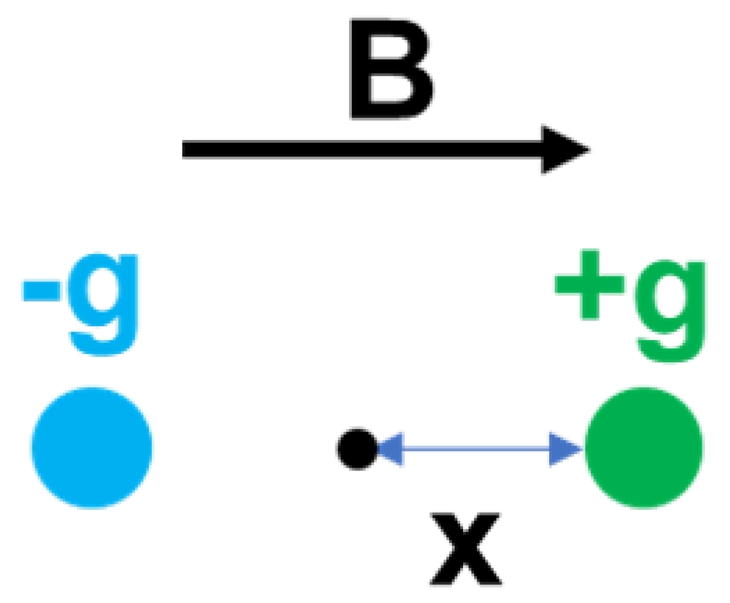
When a time-dependent A.C. magnetic field is applied to the magnetic neutral system, a parallel displacement of will take place from original equilibrium position between the opposite monopole charges, resulting in an exciton-like monopole dipole with dipole momentum , as shown in Figure 1. The motion of monopoles can be described by the damped driven oscillator model [18,19], which is written as follows:
where and is the oscillator mass and resonance frequency and is the damping constant. is the complex magnetic field. Obviously, a solution with the formation satisfies Equation (3). Therefore, we have the following:
Recall that the polarization of an electric dipole is defined as , where is the vacuum dielectric constant, the optical susceptibility, the electric dipole momentum. The magnetic polarization (magnetization) is likely , where represents the magnetization contributed from the i-th dipole in the system. Suppose the molar concentration of magnetic monopole dipole is ; hence, . Finally the magnetic susceptibility can be read as:
3. Single Magnetic Monopole in Periodic Triangle Magnetic Potential Field
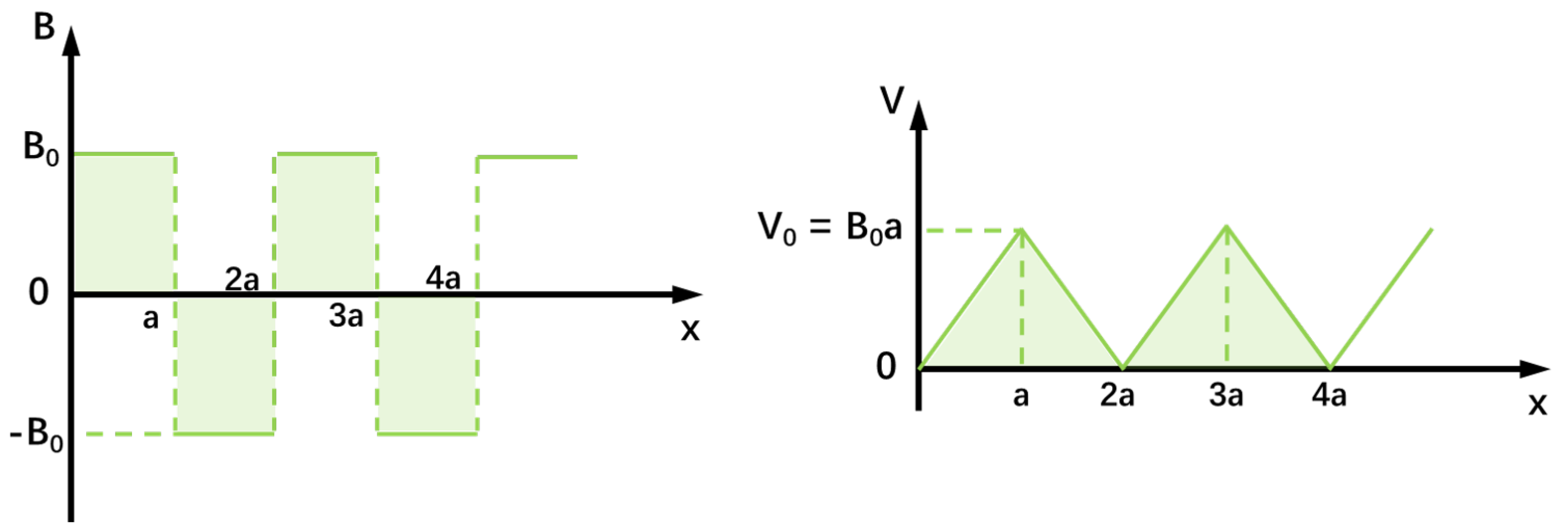
We consider in one-dimension a magnetic monopole move under an effect of a periodic uniform magnetic field. The monopole is characterized by the elementary magnetic charge g, given by the Dirac quantization condition, , where e is the elementary electron charge, h the Planck constant, and the vacuum magnetic permeability constant. The force that the monopole experiences can be written as , where is the local magnetic flux density as shown in Figure 2 left, with corresponding magnetostatic field potential V presented in the right.
The Hamiltonian of the monopole reads as follows:
where is the mass of a magnetic monopole and is the wave function. Defining the Fourier transform of a real-space wave function as , we may transform this Hamiltonian to one defined in the momentum space, as follows:
with the duality of position and momentum operators and . Since is the eigenstate of , we may write the Schrödinger equation as:
For an infinite periodic potential field, it is convenient to solve the Schrödinger equation in one single period and then use the Bloch theorem to simplify the procedure of calculating the whole wave function. Let us look at the period of . By decomposing the potential field into two segments of and , for the first segment, the problem we are confronting becomes solving the Schrödinger equation below:
This is a first-order differential equation that one can easily solve, whose answer is as follows:
For simplicity, the normalization coefficient is ignored here, while the normalization condition is . Inverse Fourier transform of Equation (10) gives the wave function in real space, which is
The right side of Equation (11) has the same form of the Airy function. By substituting variables such as and , Equation (11) becomes the standard Airy function with respect to v:
In particular, the Airy function can be expressed with the linear combination of 1/3-order Bessel functions:
in which J is the first kind of Bessel function and I is the modified Bessel function. Notably, indicates , which means the system enters the forbidden area in classical mechanism. As a result, the wave function will decay rapidly away from .
Let us now analyze the second segment where . For convenience, shifting the potential fields to the left side by a, the Schrödinger equation becomes the following:
Then, the solution of Equation (14) reads:
The wave function in real space is as follows:
where and . Substituting x with , which means that we shift the wave function back to the segment of . Finally, the wave function in one single period of can be written as , with
However, this solution only satisfies the condition of continuity, while the momentum conservation law might be broken in at the joint of opposite magnetic fields. To do this, the second Airy function needs to be introduced:
is linearly independent of with phase difference equal to ; therefore, the wave function can be expressed by the linear superposition of both Airy functions, which is as follows:
In Equation (18), are coefficients to be determined by following boundary condition:
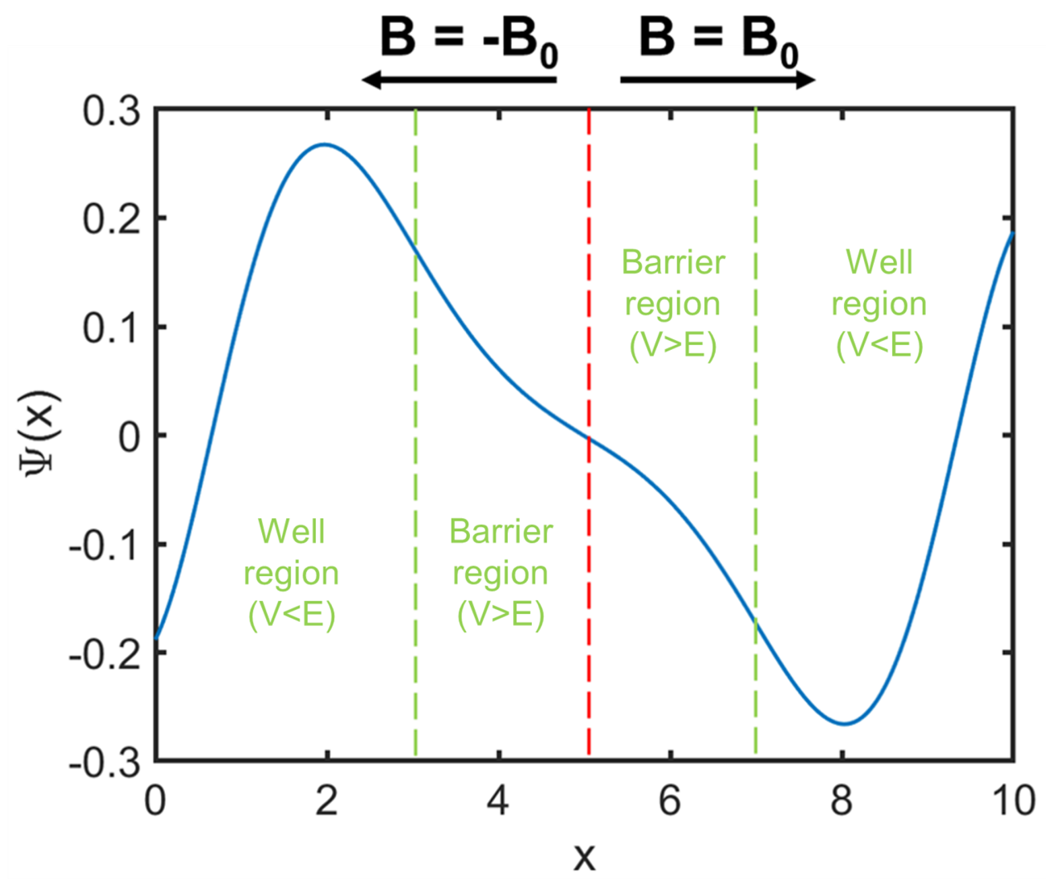
The first two equations are from the continuity of the wave function and its first derivative. The last two equations are based on the Bloch theorem where is the phase factor after the magnetic monopole traveling through one period. As we can always set one of as 1, there are four coefficients in the four equations of different boundary conditions, indicating that these coefficients can be determined by solving this equation array. In Figure 3 we show the numerical solution of the wave function under the natural unit where all constants are set to 1. The calculated pseudo-wavevector is . Finally, the wave function in the entire space reads as follows:
4. The Energy Spectrum of a Magnetic Monopole Exciton
In this section, we solve the energy spectrum of magnetic monopole exciton by considering one monopole carrying an elementary charge moving in the Coulombic potential of the opposite monopole charge g, while the Hamiltonian of a magnetic monopole exciton is quite similar to that of an electron-hole exciton or the electron in a hydrogen atom. Before doing this, we need to express the Gauss divergence theorem for a point source magnetic monopole:
This allows one to write the magnetic field as well as the field potential generated from an elementary magnetic monopole charge:
Hence, the Schrödinger equation of the motional magnetic monopole g in the monopole exciton reads:
The solution to the electron version of Equation (21) is the famous stationary wave function of electron in a hydrogen atom. Therefore, one can directly write down the eigenenergy as follows:
with the monopole Bohr radius being . Furthermore, the binding energy of a monopole exciton, , which characterizes the energy that it costs to separate the monopole exciton, can be expressed as follows:
It is well-known that the binding energy of an electron-hole pair exciton varies from meV (a Wannier-Mott exciton in an inorganic semiconductor) to several eV (a Frenkel exciton in an organic crystal) [20]. Excitons with larger binding energy are more stable. For the magnetic monopole exciton, we assume the binding energy is 2.0 eV (617 nm), one can calculate the effective mass kg from Equation (23). Besides, the process of photon emission or adsorption takes place in transitions between different energy levels m and n of monopole exciton, whose frequencies shall satisfy the following condition:
In analogue to the electron-hole exciton polariton, one can define the monopole exciton polariton as the superposition of excitonic states and photonic states, which will be discussed in the next section.
5. Magnetic Wave Equation of Monopole Exciton Polariton
In this section, we propose the model for magnetic monopole exciton-polariton, as an analogue to the conventional exciton-polariton. The coupling between the monopole exciton and the cavity photon in a microcavity system would lead to the emergence of the monopole exciton-polariton. For a static magnetic monopole, the divergence of magnetic induction intensity, , is . Using the equality of vector calculation, . While combining the Maxwell’s equation, one will have , where and are the permeability and permittivity, respectively. Notice that the relationship between magnetic induction intensity, magnetization and magnetic field is . Therefore, the constitutive equation of the magnetic field is:
where is the normalized magnetic permeability, = 1 for vacuum. Moreover, from Equation (3), one can derive the relationship between magnetization and the magnetic field:
where the extra term of comes from the kinetic energy of the magnetic monopole exciton, with being the mass of monopole exciton, the Rabi-frequency of monopole polariton. By Fourier transform, the derivative of time and space will be replaced by frequency and the momentum variable. Hence, we have the following:
The magnetic susceptibility is, then, the following:
We focus on the region near the resonant frequency ; hence, can be written as:
Using the dispersion relationship [21], , one will have . Substituting this condition to Equation (29), we find the dispersion relationship of two transverse polaritonic modes written as follows:
For the longitudinal mode of monopole polariton, the dispersion is:
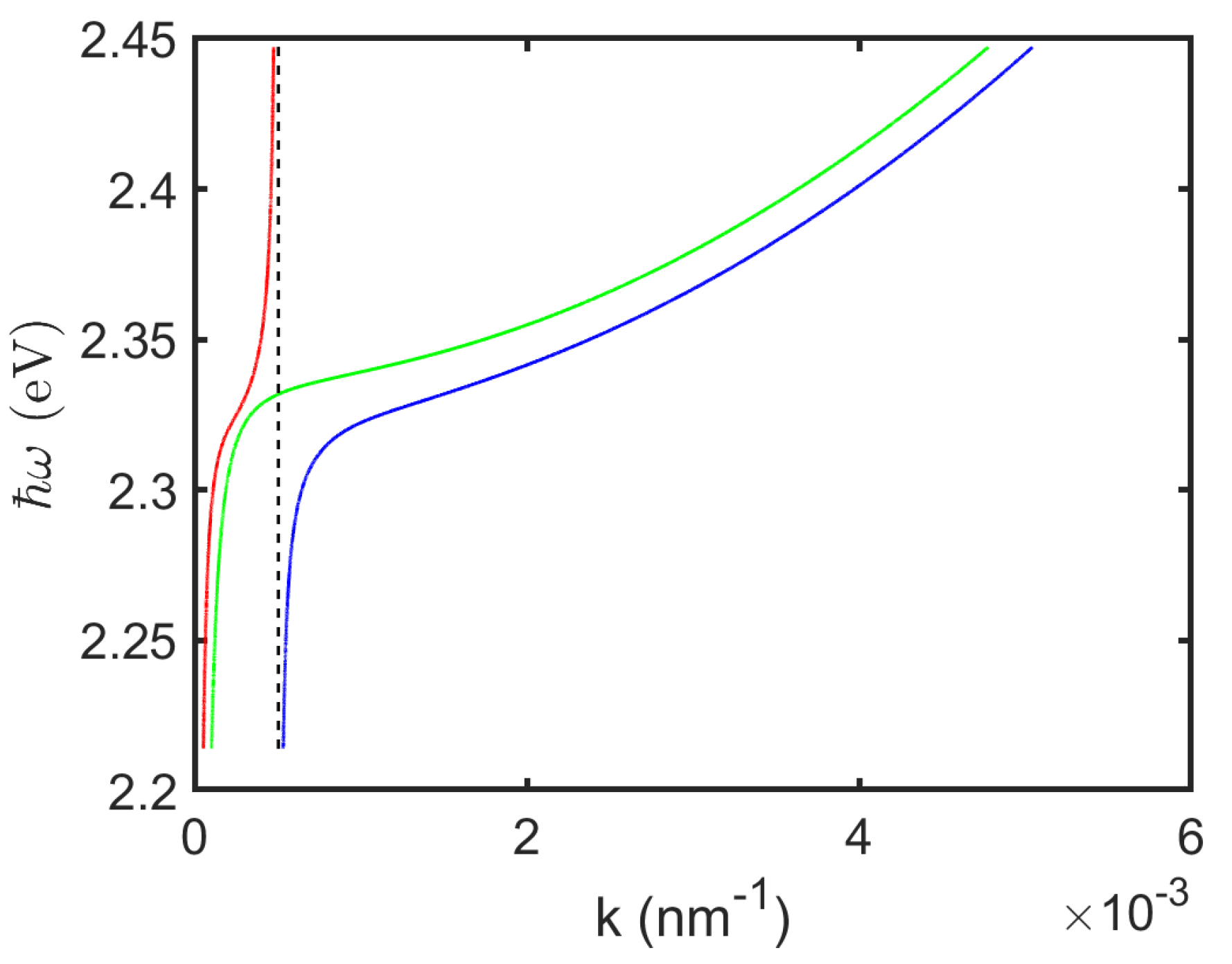
Following the previous discussion about the mass of a magnetic monopole, the parameters were taken as , , = 2.337 eV (532 nm), eV and =0.153 eV. Figure 4 shows the dispersion curves of two transverse modes (red/blue) and one longitudinal mode (green). The steepest slope of the red curve can be ascribed to the contribution of photon mode while the exciton part contributes the most to the parabolic blue curve.
The magnetic monopole exciton-polariton dispersion relationship in a microcavity system can also be performed with the well-known coupled oscillator model [22]. In general, the secular equation describing the coupling between magnetic exciton and photon could be written as follows:
where , are the frequency and broadening of the cavity mode. The off-diagonal element represents the strength of coupling. and together construct the eigen-vector of the Hamiltonian, while the eigen-energy can be solved with
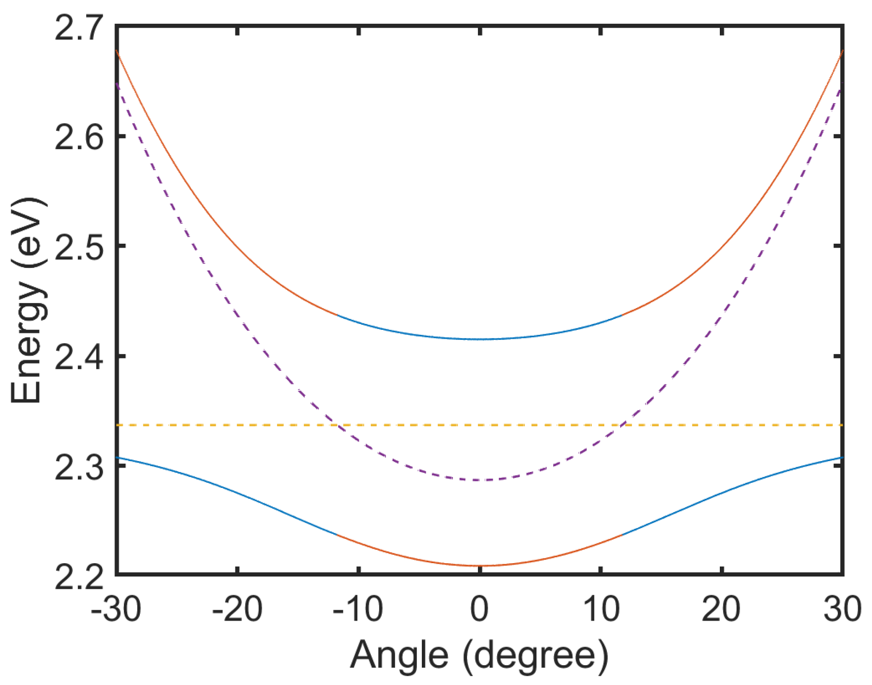
We focus on the strong coupling regime where . The definition of the strong coupling regime here is the same with that of the conventional exciton-polariton [22], where the Rabi splitting exceeds the decay rates of the magnetic monopole exciton and photon. Experiments in exciton-polariton have shown that those are tunable parameters by switching the properties such as the quality factor of the optical cavity and carrier density [19]. The dispersion curve of monopole exciton-polariton in a microcavity system, given by Equation (33), is shown in Figure 5 with parameters eV, eV, meV, meV. The inplane dispersion of exciton-polariton is plotted with solid line, while the dashed lines show the bare cavity mode and exciton mode.
6. Conclusions
In summary, we established the concept of a magnetic monopole exciton-polariton, a quasiparticle in analogue to the conventional exciton polariton, which is sensitive to the magnetic response of the system at the frequency of the external electromagnetic radiation. We used the damped driven oscillator model to analytically derive the magnetic susceptibility of a magnetic monopole under an A.C. magnetic field, and solved the Schrödinger equation of an elementary magnetic monopole in a periodic triangle potential field, which might be able to model the monopole in the periodic lattice. Specifically, we studied the energy spectrum of a magnetic monopole exciton and combined the damped oscillator model to derive the susceptibility and dispersion relationship of a monopole polariton. We believe that by placing the materials with monopole quasiparticles in optical cavities, it should be possible to optimize the systems for studies of magnetic monopole exciton-polaritons. In recent years, we have seen that the researches of exciton-polariton largely benefit the study of optics [23], quantum computation [24] and chemistry [25,26], which are also potential playgrounds for the monopole exciton-polariton.
Author Contributions
Conceptualization, A.K. and J.C.; investigation, J.C.; data curation, J.C.; writing—original draft preparation, J.C.; writing—review and editing, A.K. and J.C.; supervision, A.K. All authors have read and agreed to the published version of the manuscript.
Funding
This research was funded by Westlake University, Project 041020100118 and Program 2018R01002 by Leading Innovative and Entrepreneur Team Introduc-tion Program of Zhejiang Province of China, and Saint-Petersburg State University (Grant No. 94030557).
Data Availability Statement
The data supporting the findings of this study are available upon request.
Conflicts of Interest
The authors declare no conflict of interest.
References
- Dirac, P.A.M. Quantised singularities in the electromagnetic field. Proc. R. Soc. Lond. Ser. A Contain. Pap. Math. Phys. Character 1931, 133, 60–72. [Google Scholar] [CrossRef]
- Hooft, G. Magnetic monopoles in unified gauge theories. Nucl. Phys. B 1974, 79, 276–284. [Google Scholar] [CrossRef]
- Polyakov, A.M. Particle spectrum in quantum field theory. JETP Lett. 1974, 20, 194. [Google Scholar]
- Wu, T.T.; Yang, C.N. Some remarks about unquantized non-Abelian gauge fields. Phys. Rev. D 1975, 12, 3843–3844. [Google Scholar] [CrossRef]
- Markov, V.; Marshakov, A.; Yung, A. Non-abelian vortices in N = 1(*) gauge theory. Nucl. Phys. B 2005, 709, 267–295. [Google Scholar] [CrossRef]
- Milton, K.A. Theoretical and experimental status of magnetic monopoles. Rep. Prog. Phys. 2006, 69, 1637. [Google Scholar] [CrossRef]
- Nowakowski, M.; Kelkar, N.G. Faraday’s law in the presence of magnetic monopoles. Europhys. Lett. 2005, 71, 346. [Google Scholar] [CrossRef]
- IceCube. Search for Relativistic Magnetic Monopoles with Eight Years of IceCube Data. Phys. Rev. Lett. 2022, 128, 051101. [Google Scholar] [CrossRef]
- Jaubert, L.D.C.; Holdsworth, P.C.W. Signature of magnetic monopole and Dirac string dynamics in spin ice. Nat. Phys. 2009, 5, 258–261. [Google Scholar] [CrossRef]
- Grushin, A.G. Consequences of a condensed matter realization of Lorentz-violating QED in Weyl semi-metals. Phys. Rev. D 2012, 86, 045001. [Google Scholar] [CrossRef]
- Lv, B.Q.; Weng, H.M.; Fu, B.B.; Wang, X.P.; Miao, H.; Ma, J.; Richard, P.; Huang, X.C.; Zhao, L.X.; Chen, G.F.; et al. Experimental Discovery of Weyl Semimetal TaAs. Phys. Rev. X 2015, 5, 031013. [Google Scholar] [CrossRef]
- Vafek, O.; Vishwanath, A. Dirac Fermions in Solids: From High-Tc Cuprates and Graphene to Topological Insulators and Weyl Semimetals. Annu. Rev. Condens. Matter Phys. 2014, 5, 83–112. [Google Scholar] [CrossRef]
- Fang, Z.; Nagaosa, N.; Takahashi, K.S.; Asamitsu, A.; Mathieu, R.; Ogasawara, T.; Yamada, H.; Kawasaki, M.; Tokura, Y.; Terakura, K. The Anomalous Hall Effect and Magnetic Monopoles in Momentum Space. Science 2003, 302, 92–95. [Google Scholar] [CrossRef] [PubMed]
- Castelnovo, C.; Moessner, R.; Sondhi, S.L. Magnetic monopoles in spin ice. Nature 2008, 451, 42–45. [Google Scholar] [CrossRef] [PubMed]
- Morris, D.J.P.; Tennant, D.A.; Grigera, S.A.; Klemke, B.; Castelnovo, C.; Moessner, R.; Czternasty, C.; Meissner, M.; Rule, K.C.; Hoffmann, J.U.; et al. Dirac Strings and Magnetic Monopoles in the Spin Ice Dy2Ti2O7. Science 2009, 326, 411–414. [Google Scholar] [CrossRef] [PubMed]
- Harris, M.J.; Bramwell, S.T.; McMorrow, D.F.; Zeiske, T.; Godfrey, K.W. Geometrical Frustration in the Ferromagnetic Pyrochlore Ho2Ti2O7. Phys. Rev. Lett. 1997, 79, 2554–2557. [Google Scholar] [CrossRef]
- Ortiz-Ambriz, A.; Nisoli, C.; Reichhardt, C.; Reichhardt, C.J.O.; Tierno, P. Colloquium: Ice rule and emergent frustration in particle ice and beyond. Rev. Mod. Phys. 2019, 91, 041003. [Google Scholar] [CrossRef]
- Lorentz, H.A. The Theory of Electrons and Its Applications to the Phenomena of Light and Radiant Heat; B.G. Teubner: Leipzig, Germany, 1909. [Google Scholar]
- Kavokin, A.; Baumberg, J.; Malpuech, G. Microcavities; Oxford University Press: Oxford, UK; New York, NY, USA, 2007. [Google Scholar]
- Scholes, G.; Rumbles, G. Excitons in Nanoscale Systems. Nat. Mater. 2006, 5, 683–696. [Google Scholar] [CrossRef]
- Vladimirova, M.R.; Kavokin, A.V.; Kaliteevski, M.A. Dispersion of bulk exciton polaritons in a semiconductor microcavity. Phys. Rev. B 1996, 54, 14566–14571. [Google Scholar] [CrossRef]
- Savona, V.; Andreani, L.; Schwendimann, P.; Quattropani, A. Quantum well excitons in semiconductor microcavities: Unified treatment of weak and strong coupling regimes. Solid State Commun. 1995, 93, 733–739. [Google Scholar] [CrossRef]
- Christopoulos, S.; von Högersthal, G.B.H.; Grundy, A.J.D.; Lagoudakis, P.G.; Kavokin, A.V.; Baumberg, J.J.; Christmann, G.; Butté, R.; Feltin, E.; Carlin, J.F.; et al. Room-Temperature Polariton Lasing in Semiconductor Microcavities. Phys. Rev. Lett. 2007, 98, 126405. [Google Scholar] [CrossRef] [PubMed]
- Kavokin, A.; Liew, T.C.H.; Schneider, C.; Lagoudakis, P.G.; Klembt, S.; Hoefling, S. Polariton condensates for classical and quantum computing. Nat. Rev. Phys. 2022, 4, 435–451. [Google Scholar] [CrossRef]
- Ribeiro, R.F.; Martínez-Martínez, L.A.; Du, M.; Campos-Gonzalez-Angulo, J.; Yuen-Zhou, J. Polariton chemistry: Controlling molecular dynamics with optical cavities. Chem. Sci. 2018, 9, 6325–6339. [Google Scholar] [CrossRef]
- Fregoni, J.; Garcia-Vidal, F.J.; Feist, J. Theoretical Challenges in Polaritonic Chemistry. ACS Photonics 2022, 9, 1096–1107. [Google Scholar] [CrossRef]
Figure 1.
Magnetic field is parallel to the magnetic monopole dipole moment, displacement from equilibrium center is x.
Figure 1.
Magnetic field is parallel to the magnetic monopole dipole moment, displacement from equilibrium center is x.

Figure 2.
Profiles of magnetic field (left) and potential of monopole in the field (right).

Figure 3.
Numerical solution of the wave function of the monopole in one period of the magnetic field. The pseudo-wavevector is . The wave function is divided into barrier and well regions and shown in blue color, while the red vertical dashed line indicates the boundary where the sign of the magnetic field flips, and the green vertical dashed lines are the boundaries of barrier and well regions depending on the relationship between energy of the monopole and local potential of the magnetic field.

Figure 4.
Dispersion relationship of magnetic monopole polariton described in Equations (30) and (31), with red/blue/green curve belonging to .

Figure 5.
The coupled oscillator model of a magnetic monopole polariton in a microcavity system. Solid lines: dispersion curves of exciton-polariton. Dashed lines: non-coupled exciton (yellow) and cavity mode (purple).
Figure 5.
The coupled oscillator model of a magnetic monopole polariton in a microcavity system. Solid lines: dispersion curves of exciton-polariton. Dashed lines: non-coupled exciton (yellow) and cavity mode (purple).

Disclaimer/Publisher’s Note: The statements, opinions and data contained in all publications are solely those of the individual author(s) and contributor(s) and not of MDPI and/or the editor(s). MDPI and/or the editor(s) disclaim responsibility for any injury to people or property resulting from any ideas, methods, instructions or products referred to in the content. |
© 2023 by the authors. Licensee MDPI, Basel, Switzerland. This article is an open access article distributed under the terms and conditions of the Creative Commons Attribution (CC BY) license (https://creativecommons.org/licenses/by/4.0/).
Share and Cite
MDPI and ACS Style
Cao, J.; Kavokin, A. Optical Properties of Magnetic Monopole Excitons. Condens. Matter 2023, 8, 43. https://doi.org/10.3390/condmat8020043
AMA Style
Cao J, Kavokin A. Optical Properties of Magnetic Monopole Excitons. Condensed Matter. 2023; 8(2):43. https://doi.org/10.3390/condmat8020043
Chicago/Turabian StyleCao, Junhui, and Alexey Kavokin. 2023. "Optical Properties of Magnetic Monopole Excitons" Condensed Matter 8, no. 2: 43. https://doi.org/10.3390/condmat8020043