
Superconducting Stiffness and Coherence Length of FeSe0.5Te0.5 Measured in a Zero-Applied Field

Abstract
:1. Introduction
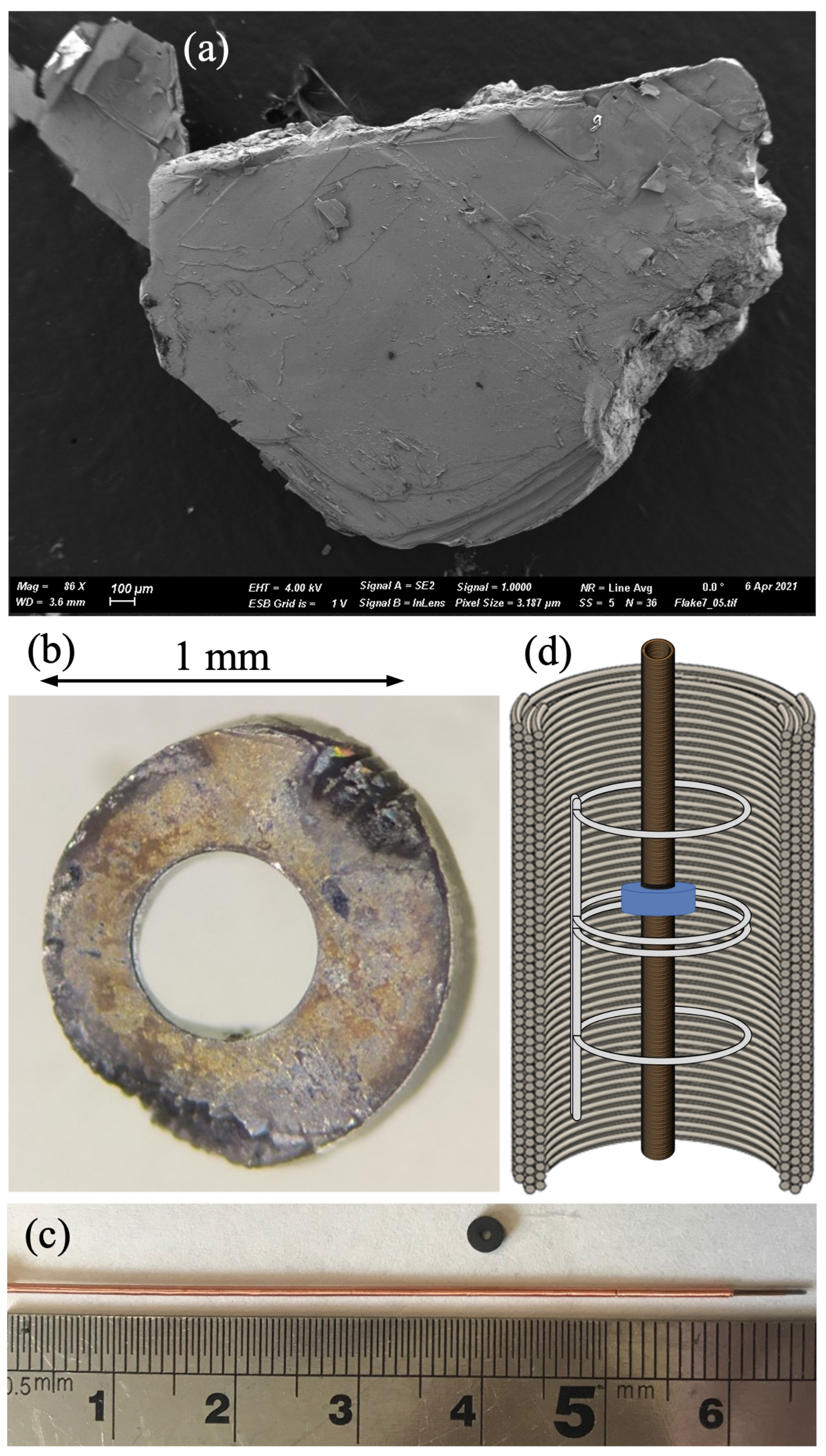
2. Experimental Setup
3. Measurements
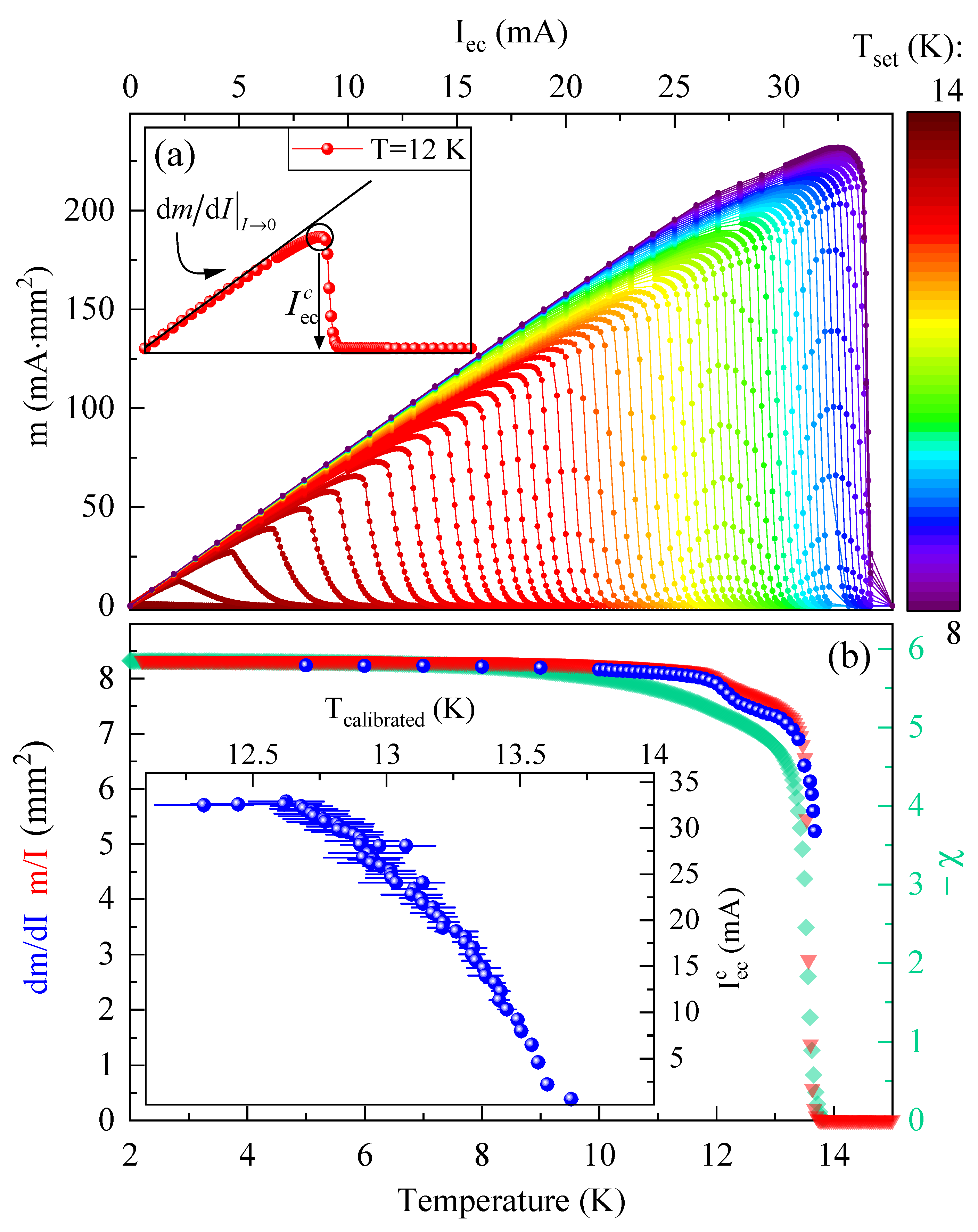
3.1. Stiffness and Critical Current
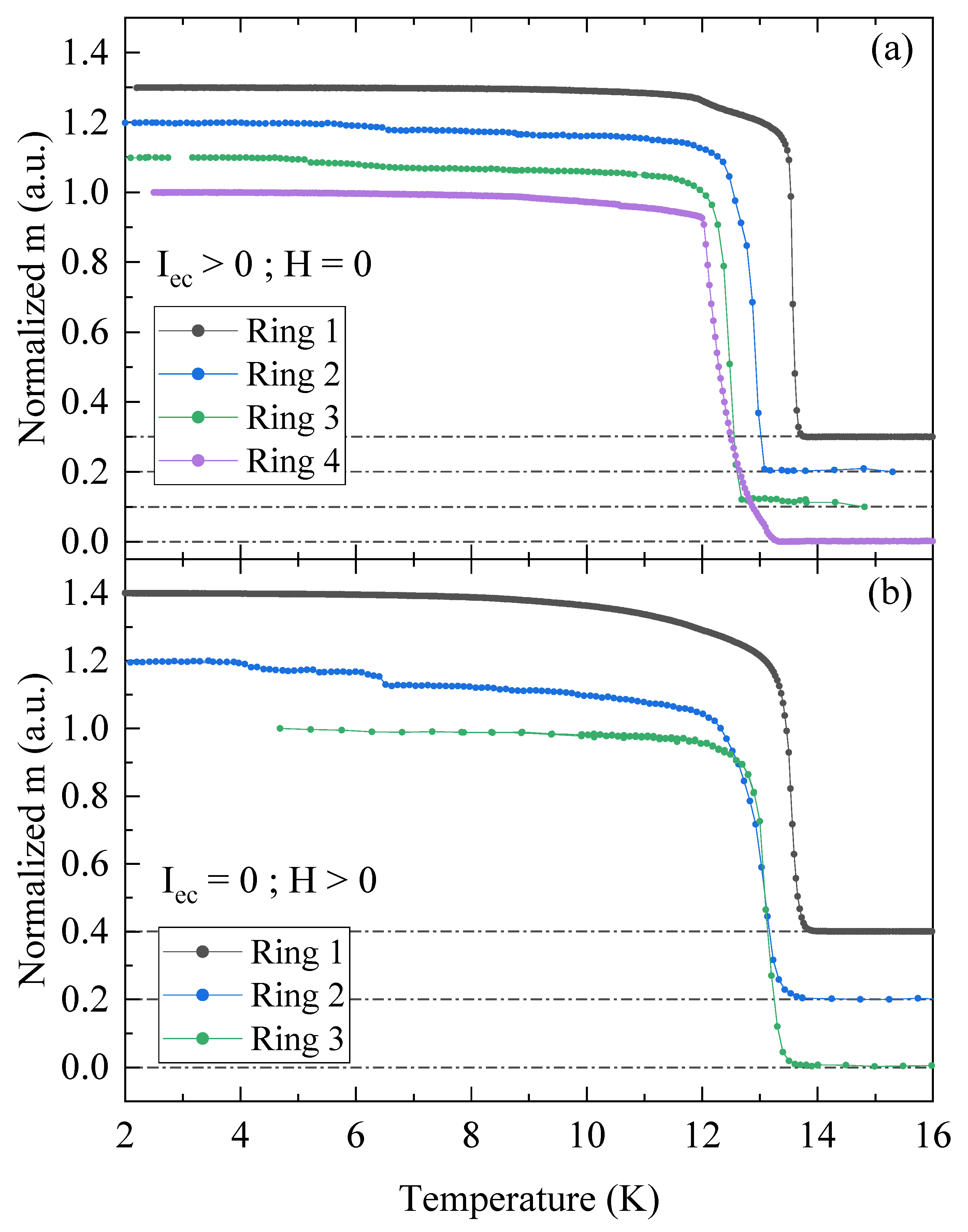
3.2. Susceptibility
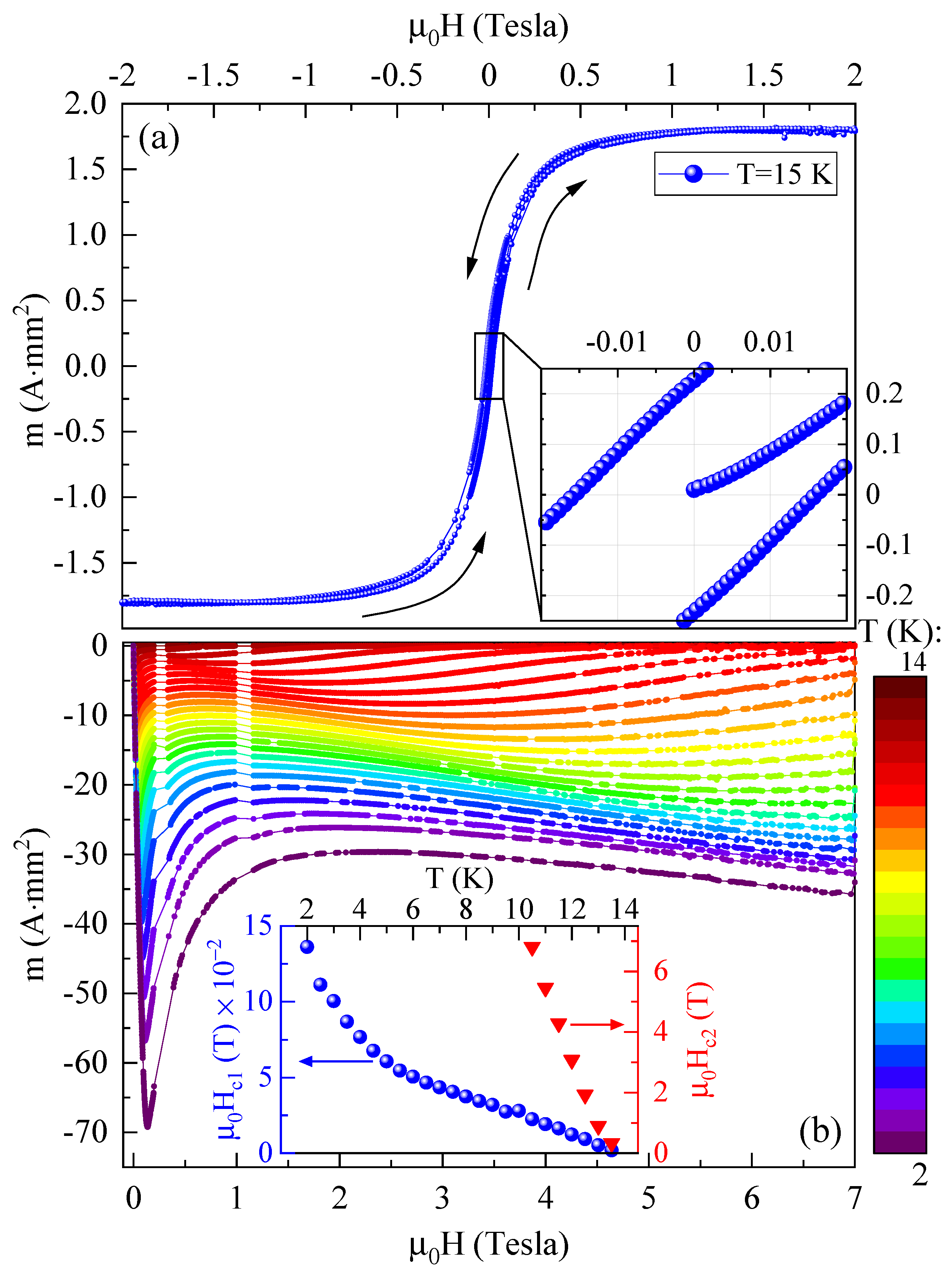
3.3. Hysteresis
3.4. Critical Magnetic Fields
4. Analysis Model
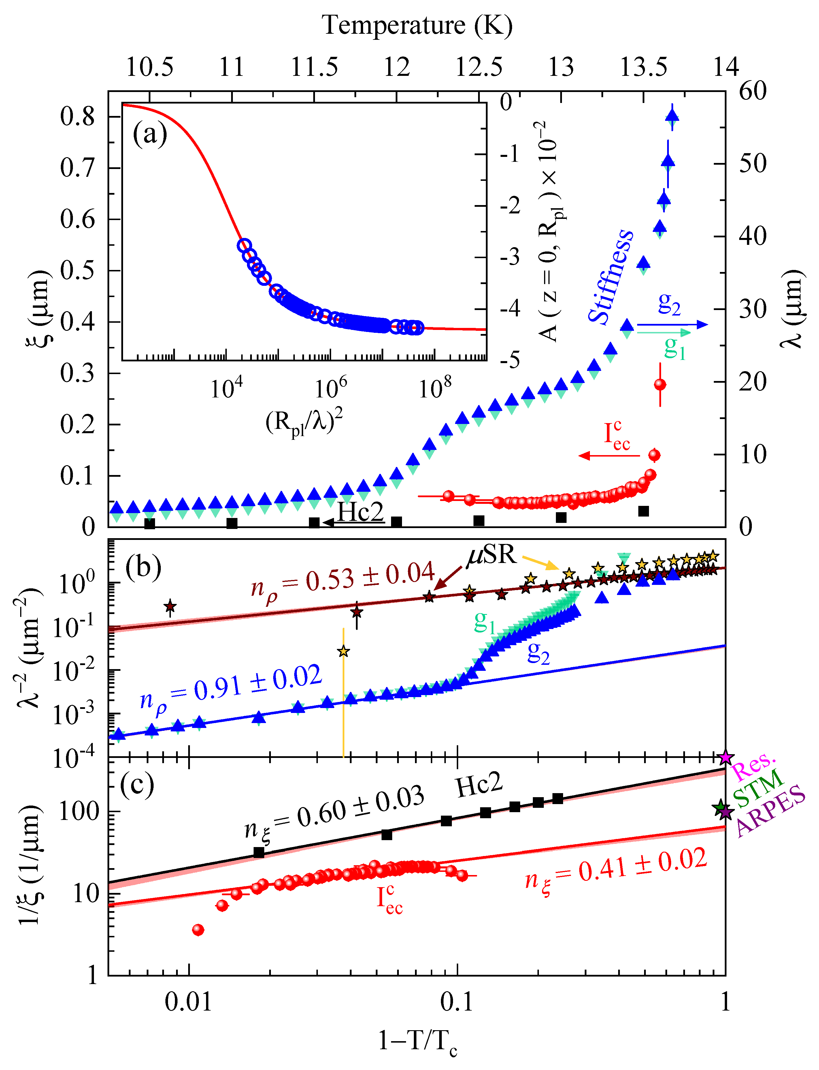
4.1. Stiffness
4.2. Coherence Length
5. Data Analysis
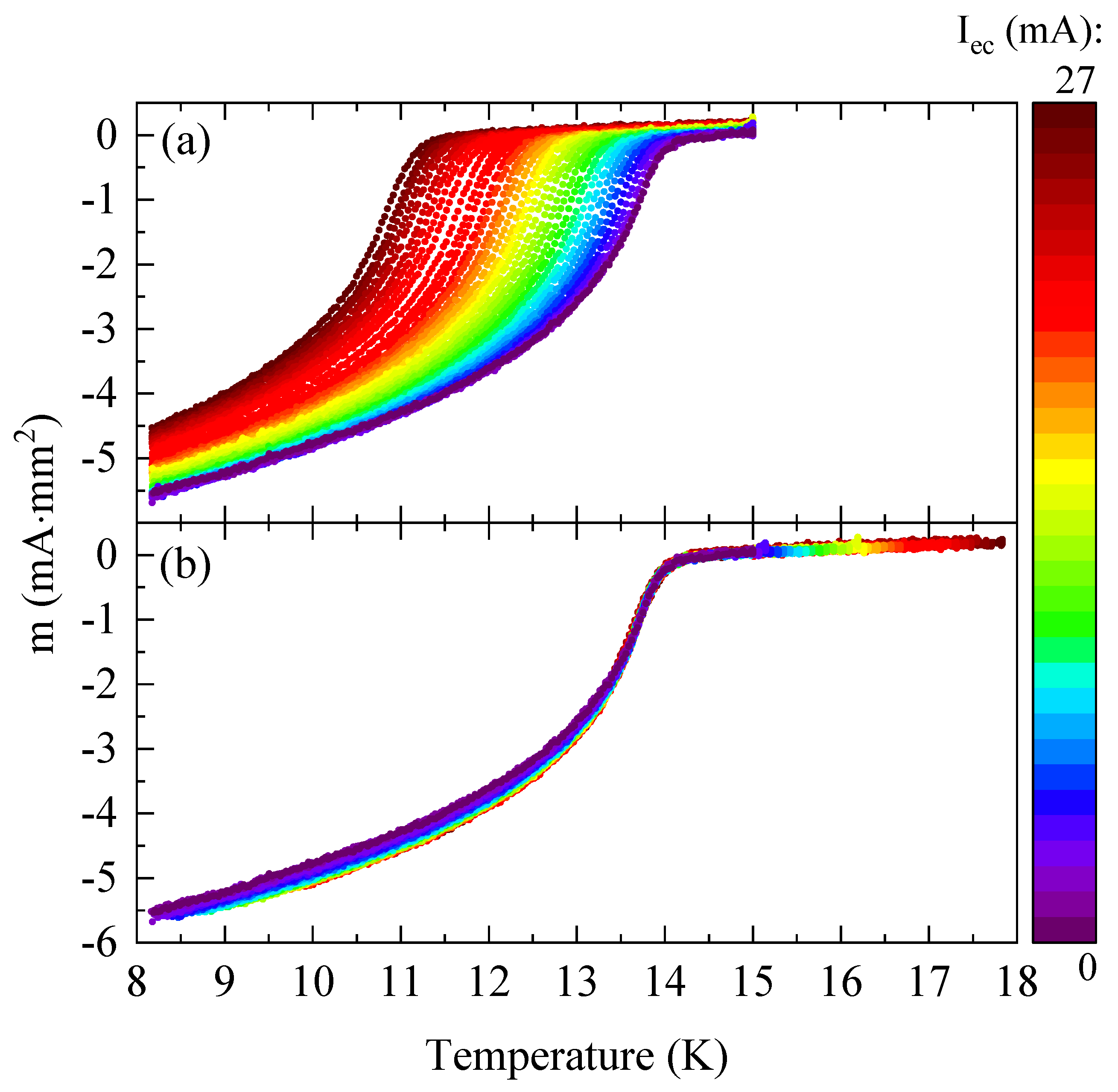
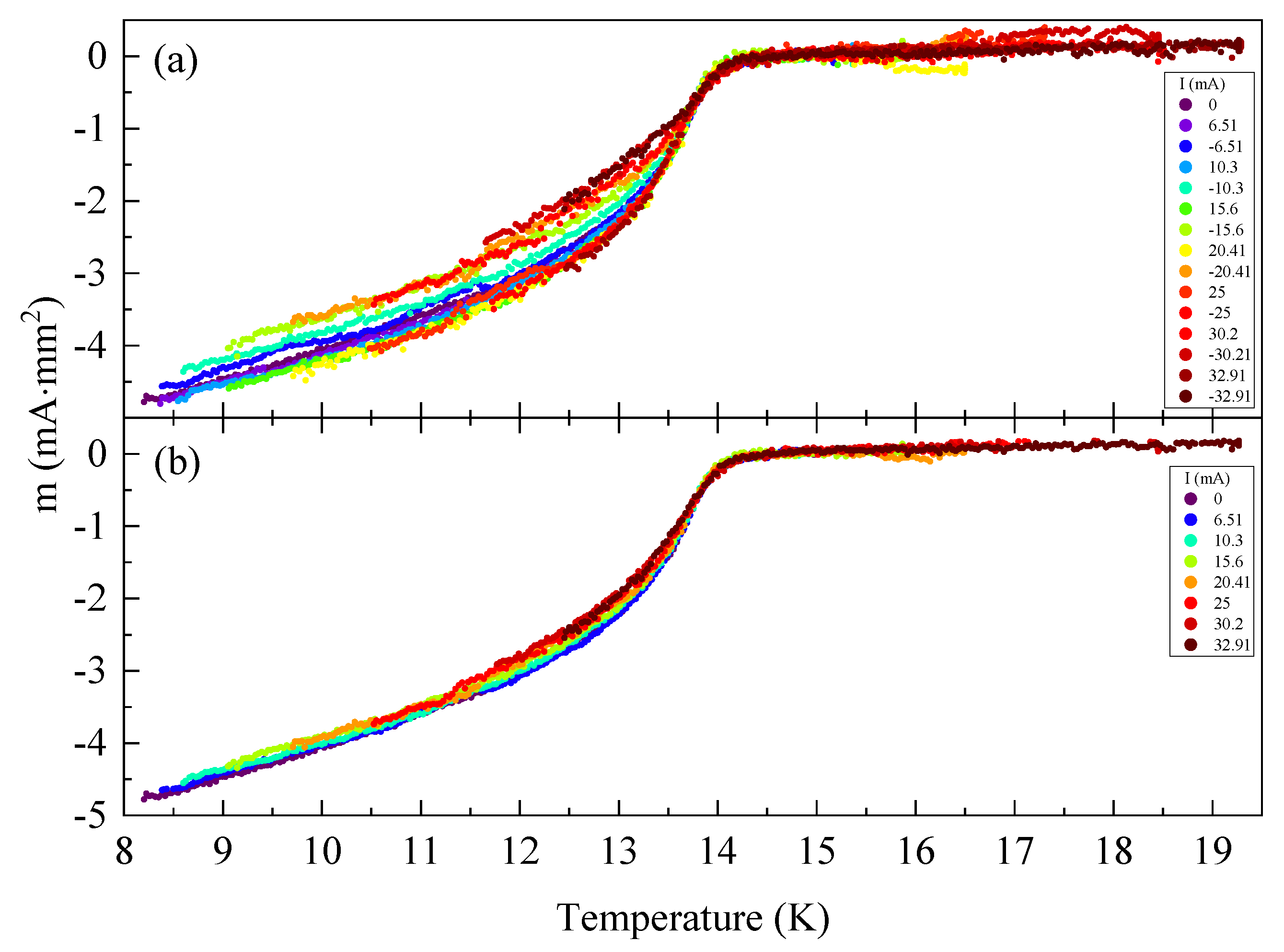
6. Reproducibility and Origin of the Knee
7. Discussion
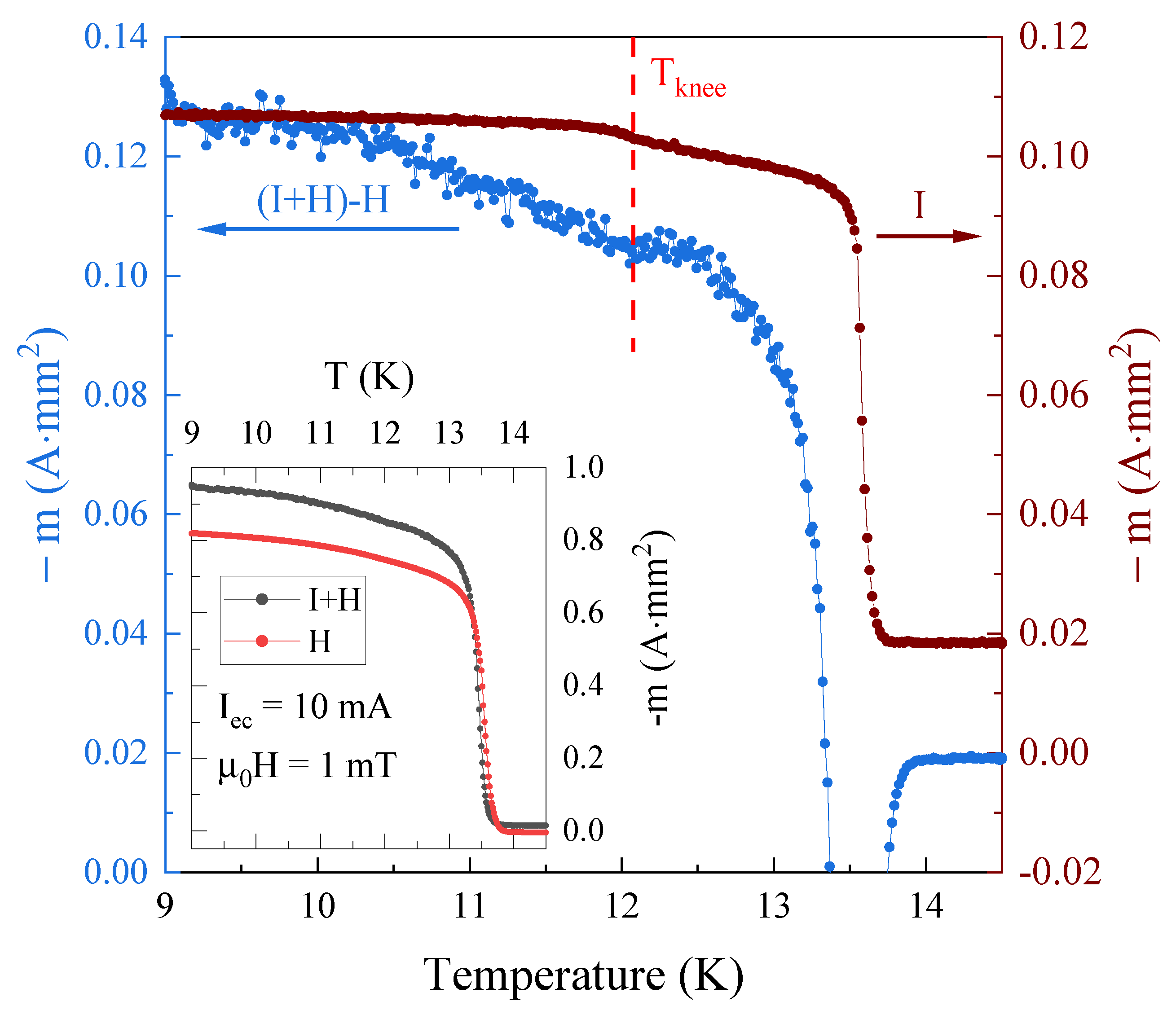
7.1. The Knee
7.2. Critical Exponents
7.3. First Critical Field
8. Conclusions
Author Contributions
Funding
Data Availability Statement
Acknowledgments
Conflicts of Interest
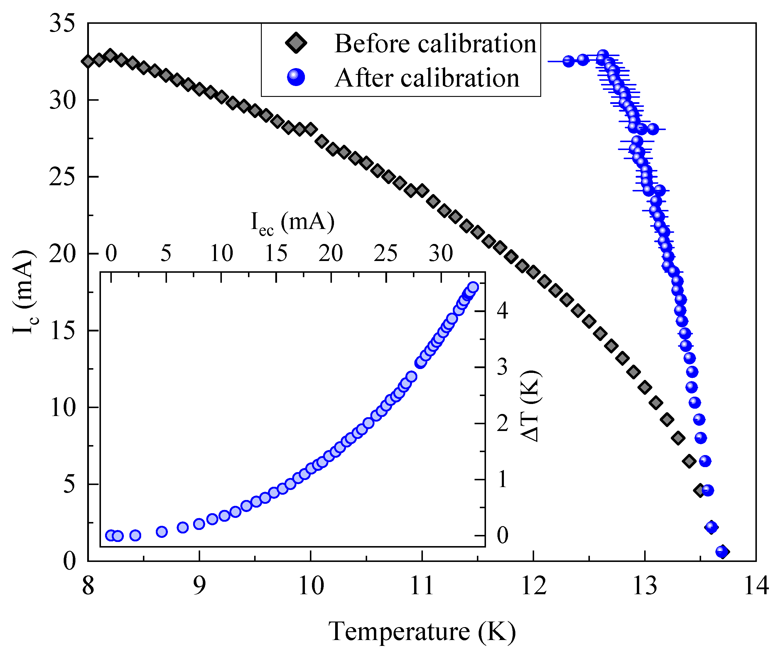
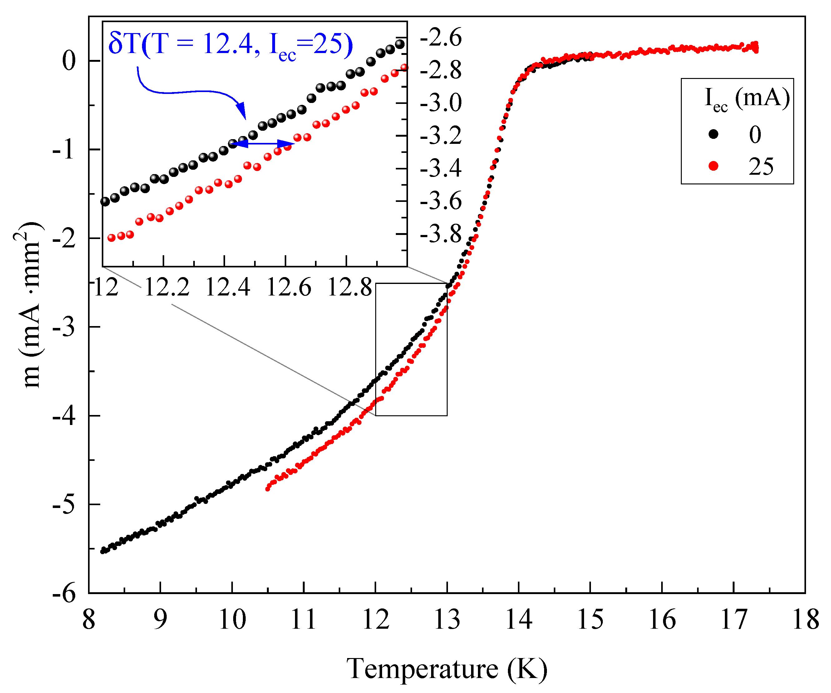
Appendix A. Temperature Calibration


References
- Wang, C.; Li, L.; Chi, S.; Zhu, Z.; Ren, Z.; Li, Y.; Wang, Y.; Lin, X.; Luo, Y.; Jiang, S.; et al. Thorium-doping-induced superconductivity up to 56 K in Gd1-xThxFeAsO. EPL (Europhys. Lett.) 2008, 83, 67006. [Google Scholar] [CrossRef]
- Kreisel, A.; Hirschfeld, P.J.; Andersen, B.M. On the remarkable superconductivity of FeSe and its close cousins. Symmetry 2020, 12, 1402. [Google Scholar] [CrossRef]
- Biswas, P.; Balakrishnan, G.; Paul, D.; Tomy, C.; Lees, M.; Hillier, A. Muon-spin-spectroscopy study of the penetration depth of FeTe0.5Se0.5. Phys. Rev. B 2010, 81, 092510. [Google Scholar] [CrossRef]
- Bendele, M.; Weyeneth, S.; Puzniak, R.; Maisuradze, A.; Pomjakushina, E.; Conder, K.; Pomjakushin, V.; Luetkens, H.; Katrych, S.; Wisniewski, A.; et al. Anisotropic superconducting properties of single-crystalline FeSe0.5Te0.5. Phys. Rev. B 2010, 81, 224520. [Google Scholar] [CrossRef]
- Serafin, A.; Coldea, A.I.; Ganin, A.; Rosseinsky, M.; Prassides, K.; Vignolles, D.; Carrington, A. Anisotropic fluctuations and quasiparticle excitations in FeSe0.5Te0.5. Phys. Rev. B 2010, 82, 104514. [Google Scholar] [CrossRef]
- Kim, H.; Martin, C.; Gordon, R.T.; Tanatar, M.A.; Hu, J.; Qian, B.; Mao, Z.Q.; Hu, R.; Petrovic, C.; Salovich, N.; et al. London penetration depth and superfluid density of single-crystalline Fe1+yTe1-xSex and Fe1+yTe1-xSx. Phys. Rev. B 2010, 81, 180503. [Google Scholar] [CrossRef]
- Takahashi, H.; Imai, Y.; Komiya, S.; Tsukada, I.; Maeda, A. Anomalous temperature dependence of the superfluid density caused by a dirty-to-clean crossover in superconducting FeSe0.4Te0.6 single crystals. Phys. Rev. B 2011, 84, 132503. [Google Scholar] [CrossRef]
- Kurokawa, H.; Nakamura, S.; Zhao, J.; Shikama, N.; Sakishita, Y.; Sun, Y.; Nabeshima, F.; Imai, Y.; Kitano, H.; Maeda, A. Relationship between superconductivity and nematicity in FeSe1-xTex(x=0-0.5) films studied by complex conductivity measurements. Phys. Rev. B 2021, 104, 014505. [Google Scholar] [CrossRef]
- Wang, D.; Kong, L.; Fan, P.; Chen, H.; Zhu, S.; Liu, W.; Cao, L.; Sun, Y.; Du, S.; Schneeloch, J.; et al. Evidence for majorana bound states in an iron-based superconductor. Science 2018, 362, 333. [Google Scholar] [CrossRef]
- Shruti, G. Sharma, S. Patnaik. Anisotropy in upper critical field of FeTe0.55Se0.45. AIP Conf. Proc. 2015, 1665, 130030. [Google Scholar] [CrossRef]
- Chiu, C.-K.; Machida, T.; Huang, Y.; Hanaguri, T.; Zhang, F.-C. Scalable majorana vortex modes in iron-based superconductors. Sci. Adv. 2020, 6, eaay0443. [Google Scholar] [CrossRef]
- Kapon, I.; Salman, Z.; Mangel, I.; Prokscha, T.; Gavish, N.; Keren, A. Phase transition in the cuprates from a magnetic-field-free stiffness meter viewpoint. Nat. Commun. 2019, 10. [Google Scholar] [CrossRef]
- Gavish, N.; Kenneth, O.; Keren, A. Ginzburg–Landau model of a stiffnessometer—A superconducting stiffness meter device. Phys. Nonlinear Phenom. 2021, 415, 132767. [Google Scholar] [CrossRef]
- Mangel, I.; Kapon, I.; Blau, N.; Golubkov, K.; Gavish, N.; Keren, A. Stiffnessometer: A magnetic-field-free superconducting stiffness meter and its application. Phys. Rev. B 2020, 102, 024502. [Google Scholar] [CrossRef]
- Keren, A.; Blau, N.; Gavish, N.; Kenneth, O.; Ivry, Y.; Suleiman, M. Stiffness and coherence length measurements of ultra-thin superconductors, and implications for layered superconductors. Supercond. Sci. Technol. 2022, 35, 075013. [Google Scholar] [CrossRef]
- Beleggia, M.; Vokoun, D.; Graef, M.D. Demagnetization factors for cylindrical shells and related shapes. J. Magn. Magn. Mater. 2009, 321, 1306. [Google Scholar] [CrossRef]
- Farhang, C.; Zaki, N.; Wang, J.; Gu, G.; Johnson, P.D.; Xia, J. Revealing the origin of time-reversal symmetry breaking in fe-chalcogenide superconductor FeTe1-xSex. Phys. Rev. Lett. 2023, 130, 046702. [Google Scholar] [CrossRef]
- Weiss, A. Magnetic Oxides, Part 1 + 2; Craik, D.J., Ed.; JW Wiley & Sons: London, UK; New York, NY, USA; Sydney, Australia; Toronto, ON, Canada, 1975. [Google Scholar]
- Wang, J.; Bao, S.; Shangguan, Y.; Cai, Z.; Gan, Y.; Li, S.; Ran, K.; Ma, Z.; Winn, B.L.; Christianson, A.D.; et al. Enhanced low-energy magnetic excitations evidencing the Cu-induced localization in the Fe-based superconductor Fe0.98Te0.5Se0.5. Phys. Rev. B 2022, 105, 245129. [Google Scholar] [CrossRef]
- Galluzzi, A.; Buchkov, K.; Tomov, V.; Nazarova, E.; Leo, A.; Grimaldi, G.; Nigro, A.; Pace, S.; Polichetti, M. Evidence of pinning crossover and the role of twin boundaries in the peak effect in FeSeTe iron based superconductor. Supercond. Sci. Technol. 2017, 31, 015014. [Google Scholar] [CrossRef]
- Tinkham, M. Introduction to Superconductivity; Courier Corporation: Chelmsford, MA, USA, 2004. [Google Scholar]
- Hecht, F. New development in FreeFem++. J. Numer. Math. 2012, 20, 251. [Google Scholar] [CrossRef]
- Varmazis, C.; Strongin, M. Inductive transition of niobium and tantalum in the 10-MHz range. I. zero-field superconducting penetration depth. Phys. Rev. B 1974, 10, 1885. [Google Scholar] [CrossRef]
- Mukasa, K.; Matsuura, K.; Qiu, M.; Saito, M.; Sugimura, Y.; Ishida, K.; Otani, M.; Onishi, Y.; Mizukami, Y.; Hashimoto, K.; et al. High-pressure phase diagrams of FeSe1-xTex: Correlation between suppressed nematicity and enhanced superconductivity. Nat. Commun. 2021, 12, 1. [Google Scholar] [CrossRef] [PubMed]
- Zhang, P.; Yaji, K.; Hashimoto, T.; Ota, Y.; Kondo, T.; Okazaki, K.; Wang, Z.; Wen, J.; Gu, G.; Ding, H.; et al. Observation of topological superconductivity on the surface of an iron-based superconductor. Science 2018, 360, 182. [Google Scholar] [CrossRef] [PubMed]
- De Gennes, P.-G.; Pincus, P.A. Superconductivity of Metals and Alloys; CRC Press: Boca Raton, FL, USA, 2018. [Google Scholar]
- Sajilesh, K.P.; Singh, D.; Biswas, P.K.; Hillier, A.D.; Singh, R.P. Superconducting properties of the noncentrosymmetric superconductor LaPtGe. Phys. Rev. B 2018, 98, 214505. [Google Scholar] [CrossRef]
- Shang, T.; Amon, A.; Kasinathan, D.; Xie, W.; Bobnar, M.; Chen, Y.; Wang, A.; Shi, M.; Medarde, M.; Yuan, H.; et al. Enhanced Tc and multiband superconductivity in the fully-gapped ReBe22 superconductor. N. J. Phys. 2019, 21, 073034. [Google Scholar] [CrossRef]


Disclaimer/Publisher’s Note: The statements, opinions and data contained in all publications are solely those of the individual author(s) and contributor(s) and not of MDPI and/or the editor(s). MDPI and/or the editor(s) disclaim responsibility for any injury to people or property resulting from any ideas, methods, instructions or products referred to in the content. |
© 2023 by the authors. Licensee MDPI, Basel, Switzerland. This article is an open access article distributed under the terms and conditions of the Creative Commons Attribution (CC BY) license (https://creativecommons.org/licenses/by/4.0/).
Share and Cite
Peri, A.; Mangel, I.; Keren, A. Superconducting Stiffness and Coherence Length of FeSe0.5Te0.5 Measured in a Zero-Applied Field. Condens. Matter 2023, 8, 39. https://doi.org/10.3390/condmat8020039
Peri A, Mangel I, Keren A. Superconducting Stiffness and Coherence Length of FeSe0.5Te0.5 Measured in a Zero-Applied Field. Condensed Matter. 2023; 8(2):39. https://doi.org/10.3390/condmat8020039
Chicago/Turabian StylePeri, Amotz, Itay Mangel, and Amit Keren. 2023. "Superconducting Stiffness and Coherence Length of FeSe0.5Te0.5 Measured in a Zero-Applied Field" Condensed Matter 8, no. 2: 39. https://doi.org/10.3390/condmat8020039