
Conductivity Sum Rule in the Nearly Free Two-Dimensional Electron Gas in an Uniaxial Potential

Department of Physics, Faculty of Science, University of Zagreb, Bijenička 32, 10000 Zagreb, Croatia
*
Author to whom correspondence should be addressed.
Condens. Matter 2023, 8(1), 1; https://doi.org/10.3390/condmat8010001
Submission received: 17 November 2022
/
Revised: 13 December 2022
/
Accepted: 20 December 2022
/
Published: 23 December 2022
(This article belongs to the Special Issue Selected Papers from the International Conference on Quantum Materials and Technologies (ICQMT2022))
Abstract
:We report an investigation of the conductivity sum rule in the two-dimensional system of free electrons in a weak uniaxial potential. The sum rule is defined through the integration of a real part of a multiband conductivity tensor and separates between the intraband and interband charge transport concentrations. It is shown how the relative direction of the electric field and the uniaxial potential defines the transport concentrations of the nearly free electron system and why the sum rule is obeyed.
1. Introduction
The conductivity sum rule is an important tool in the analysis of the dynamical charge transport properties in the strongly correlated systems [1,2]. In this paper, we show, by using the simple electron gas model exposed to periodic potential on the atomic scale, how the electron transport concentrations (which are of fundamental importance in experimental data analysis), depend on doping under conditions of the pseudogap formation. Due to the presence of multiple electron-scattering channels and a significant number of bands around Fermi level, it is a challenge to separate intraband from interband contributions in the dynamical conductivity measurements. We demonstrate the sum rule connection with the charge conservation in the two-dimensional (2D) system of nearly free electrons (NFE) in an additional weak periodic potential. We assume that the weak periodic potential is uniaxial, having a single Fourier component with amplitude and the modulation wave vector , and that the Fermi energy can be easily changed. A possible onset of such potential in the real system is stabilization of the charge density wave (CDW). Hence, we call this model by abbreviation UniAxNFE. The conservation of charge that participates in electric transport, or the sum rule, amounts to evaluating the contributions from partial spectral weights which originate from the real parts of the intraband and interband conductivity. The general form of the multiband conductivity tensor [3] is approximated by an expression consisting of a bare single-particle electron-hole energies and a phenomenological electron-hole scattering constant. This approximate form of the multiband conductivity tensor is then divided into its intra- and interband parts, which are then evaluated in the long wavelength limit of a perturbating electric field. In this way, we obtain a simple form of the intraband part of the multiband conductivity tensor, known as the Drude conductivity formula [4], whereas the contributions to the conductivity originating from the interband excitations, will be referred to as optical conductivity [5]. In the limit of the vanishing intra- and interband relaxation constant, the expressions for the real parts of intra- and interband conductivity become simplified and, for the particular model of the electron ground state used in this work, they are given in a closed form. The sum rule is defined in Ref. [6] as well as the way by which it connects the real part of the conductivity and the various types of electron transport concentrations. The latter depends on the direction in which the macroscopic electric field is pointing.
The electron energies of the resulting two-band UniAxNFE model [4,7] retain, to some extent, the free electron-like properties in the direction perpendicular to , whereas in the parallel direction, the bands are strongly influenced by the potential; hence, as a result a pseudogap is opened. The pseudogap position and its width is defined by two of the four characteristic energy points of the electron bands. These points also define the intervals of different energy dependence of the transport concentrations. Finally, we explicitly show how we can identify the intraband and interband effective electron concentration of the UniAxNFE model, which when added together, yield the total charge concentration. Moreover, we demonstrate a different energy dependence of these effective transport concentrations when measured in the direction parallel to the wave vector , and direction perpendicular to it.
2. Multiband Conductivity Tensor
Here we give a simple overview of the general form of the conductivity tensor in a simple cubic type of crystal without the infrared active phonons. The conductivity tensor includes contributions from all types of single-particle excitation in a multiband system. Within the linear response theory, the conductivity tensor [3] is defined as a connection between the Cartesian component of the induced current density with respect to the same component of the macroscopic electric field,
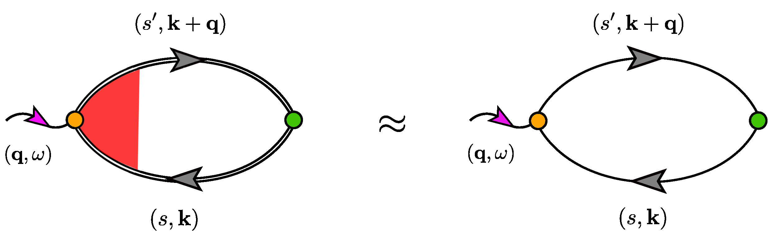
where are the wave vector and frequency of the macroscopic electric field . In its general form, as shown in Figure 1, the conductivity tensor is in fact a current-dipole correlation function. This object is too complicated to be used as a tool for a simple analysis of the dynamical transport properties, so a simplified version has to be introduced. In this simplification of the conductivity tensor [8], the electron and hole self-energy renormalisation is neglected and electron-hole scattering is approximated by the phenomenological constant , which depends on the band index s,
In (2), is the s-band energy with the corresponding Fermi–Dirac distribution , V is the volume (area) of the crystal. The first term within the -summation, which extends over the first Brillouin zone in (2), is a product of current and dipole matrix elements, which are connected via continuity equation [10]. This is why the product of current and dipole matrix elements is written by using just the current elements () and the single-particle energies. Thus, is the matrix element of an -dependent matrix , which is derived by using the unitary matrix needed to diagonalize the electron Hamiltonian and the derivative of the Hamiltonian matrix [7,8,11],
In general, the intraband current matrix elements are model-independent and given by
whereas the interband (s ≠ s′) current matrix elements are model-dependent. Taking the q→0 limit in the Equation (2) and dividing it in the intraband (s = s′) and interband (s ≠ s′) channel and assuming that the intraband phenomenological relaxation constants are equal to γ we get
In Equation (5), we have introduced the effective concentrations of electrons that participate in the intraband transport [12]. There are two equivalent forms of [13] obtainable from one another by partial integration,
We now turn to the real part of the total conductivity tensor (5) in the limit of a vanishing relaxation constants . For the intraband conductivity, we obtain
and, correspondingly, for the interband conductivity,
The sum rule states that by integrating the real part of the conductivity (7) and (8), which are even function of ω, he conserved quantity called the spectral weight is obtained [6,12,14],
where we have defined, analogously to the intraband effective concentration of electrons (6),
an interband effective concentration of electrons
For any multiband system, the sum rule (9) states that the concentration of electrons engaged in the dynamical charge transport is distributed among electrons participating in the intraband, and those participating in the interband excitations,
Here, we stress that can be different from the total concentration of electrons needed to fill the bands up to the Fermi energy. Whether or not and are equal, depends on the electron model in question. We will show that for the UniAxNFE model indeed . This, however, does not apply for the systems with linear electron dispersions like the d-dimensional Dirac systems [3,15,16] where . Moreover, evaluating the relation (6a) for the single-band system described by , we can easily obtain the following general relation:
Thus, we see that only for the parabolic-like electron dispersion (), and might be equal. We now turn our attention to the example of the two-band system in which (11) is conserved.
3. Two-Dimensional UniAxNFE Model
As a testing ground for the sum rule (9), we analyze the charge transport properties of the two-dimensional, nearly free electron gas in the presence of weak periodic uniaxial potential. The crystal potential is of the form with the wave vector , thus becoming the new reciprocal lattice vector. The electronic two-band Hamiltonian in its matrix form in the basis of and , where the latter are the states near a single Bragg’s plane defined by , is
where where , is electron wave vector, is the bare electron mass [4]. The diagonalisation of Equation (13) gives two electron bands labeled by index within the newly defined Brillouin zone with the periodicity determined by ,
In the electron dispersion Equation (14), is defined relatively to by decomposition where is parallel to the -direction. Moreover, the origin of the newly formed Brillouin zone is shifted by . Implementing these changes in Equation (14), we get
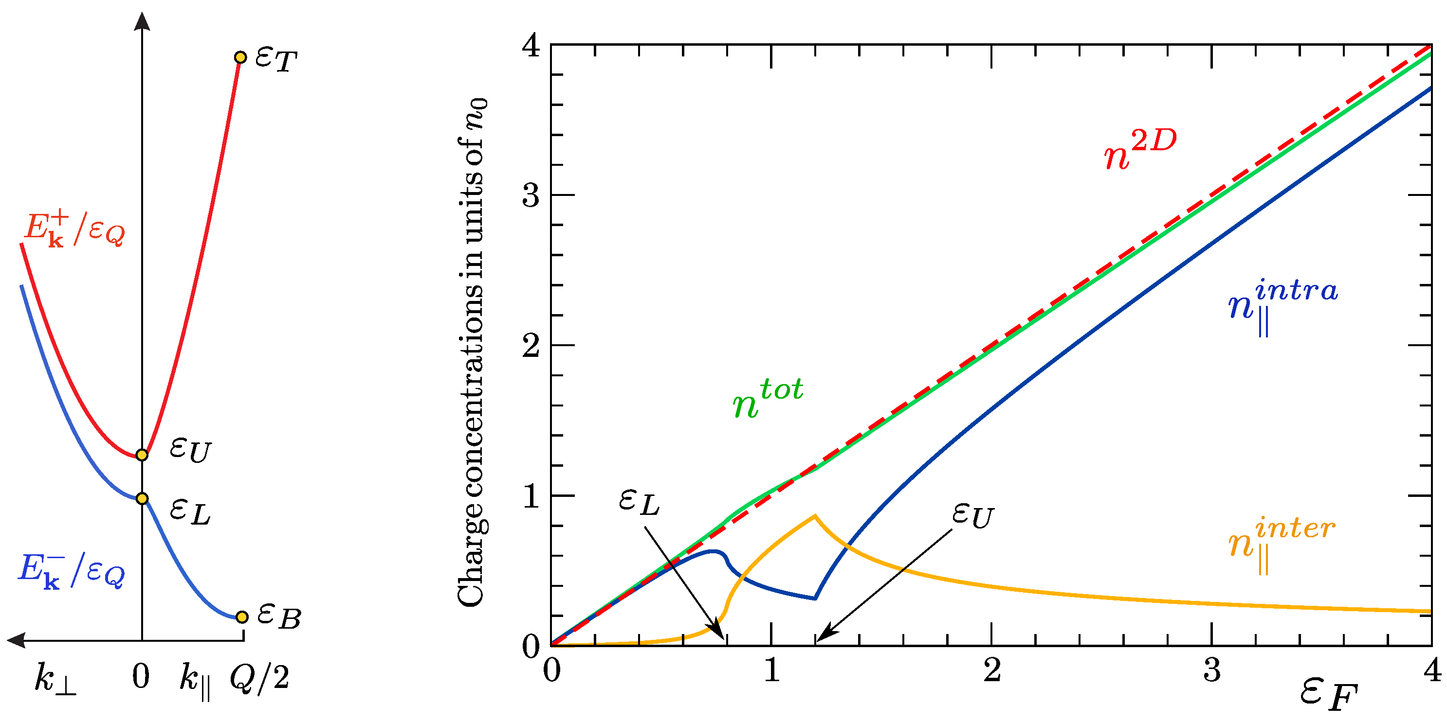
The two electron dispersions (15) are shown in Figure 2 (left) and are scaled with the , the electron energy at the Bragg’s plane, where the dispersions cross, prior to the pseudogap opening. In addition, a dimensionless gap parameter is introduced as a dimensionless order parameter, i.e., the measure of strength of the periodic potential. In the weak periodic potential approach we expect . The Brillioun zone, over which Equation (15) is spanned, resembles an infinitely long stripe in direction of total width . Four characteristic energy points related to the bands (15) are identified and designated by the yellow circle in Figure 2. The bottom (B) energy of the band and the top (T) energy of the band, within the cross-section of the Brillouin zone, are located at (see Figure 2 (left)). We have
In addition, the extent of the pseudogap region at is determined by the upper (U) and lower (L) energy
Calculated properties related to the charge transport will be presented as functions of the scaled Fermi energy .
4. Charge Transport Concentrations of the 2D UniAxNFE Model
Dispersion (15) implies different response to the dynamical electric field pointing parallel, or perpendicular to the direction of the vector . To demonstrate this, we calculate the intraband concentration (6), for electrons described by the bands (15), filed up to the scaled Fermi energy at zero temperature for two distinct directions .
Let us inspect the ⊥ direction first. It is easy to check from (15) that , and thus Equation (6b) reduces to the standard definition of the total concentration of electrons ,
which is shown in Figure 2 (right) in green as a function of in units of concentration . should be compared to the total concentration of 2D free electrons which is
and is shown as a red dashed line in Figure 2 (right). We see a small deviation between the two concentrations (18) and (19) within the pseudogap region and for high values. This illustrates a small but observable influence of the uniaxial potential on the transport in the perpendicular direction. Moreover, from the Hamiltonian (13) and from the definition of the current matrix elements (4), we can derive [7] the interband current matrix elements
The only Cartesian component , for which (20) is finite, is . By inspecting Equation (10), we conclude that the interband concentration of electrons is
Therefore, the interband conductivity in the electron model derived in Section 3 is finite only when the macroscopic electric field is applied in the direction parallel to the vector . Comparing expressions (21), (18) and (11), we get
If the macroscopic electric field is oriented parallel to , the calculated is shown in Figure 2 (right) in blue. As is seen for , the two concentrations and nearly coincide. The biggest difference between them is when is within the pseudogap region . The is calculated by inserting (20) into Equation (10). The result is also shown in Figure 2 (right) in orange. The main feature of is that it is nearly zero for and that it has a maximum at . Furthermore, by inspecting the Figure 2 (right), we observe that
The above expression can be shown explicitly by adding the terms in (6b) and (10) with (20) together under the same .
Another way of showing that a simple two-band model (15) obeys the sum rule (23) is by integrating the real part of the optical conductivity. To demonstrate this, we plot the parallel component of the real part of the interband conductivity which for the present model, has been derived in [7],
In the above expression, is the scaled photon energy , and is the Heaviside unit step function and is the two-dimensional conductivity constant. Equation (24) is plotted in Figure 3 (left) for three values of whose positions are indicated by correspondingly colored arrows on the right part of Figure 3. Expression (24) is finite only for frequencies within the interval as shown in Figure 3. These limits originate from the energy conservation (8) with bands (15) that are spanned between the endpoints (16). Moreover, if , then (blue curve) is finite, whereas if , then develops a one-over a square-root type of divergence (red and dashed green line Figure 3 (left)). The common feature of the Equation (24) is the decay as we increase . Using as the new frequency variable, Equation (9) gives
Because of the -restrictions in the , the upper limit in the integral is set to . After finding the area under the conductivity curve numerically, as noted by the shaded region of the blue curve in Figure 3 (left), we obtain as shown in the Figure 2 (right).
As mentioned, the approach where we simply equate , does not apply for the 2D or 3D Dirac system [16,17] where the interband current matrix elements (20) are constant for any , and correspondingly, . In order to apply the sum rule (9) with , a cutoff frequency has to be introduced in the upper boundary of the integral in (25) to prevent from diverging. This will in turn lead to a self-consistency problem in which the parameters, like the Fermi energy , will be tied to .
5. Conclusions
We have identified main parts of the multiband conductivity tensor within the single loop approximation and with a constant electron-hole scattering constant. After dividing the real part of the conductivity tensor to the intraband and interband parts we have applied the sum rule and obtained the intraband and interband charge concentrations. These charge concentrations that depend on the direction of an applied electric field where calculated for a simple two-dimensional, nearly free electron gas in a weak uniaxial crystal potential described by a two-band model. One possible way to introduce such a periodic potential, varying on an atomic scale, into the nearly free electron system is an onset of the charge density wave, for which several mechanisms has been proposed [18,19,20]. All aspects of eventual coherent CDW dynamics are neglected in this consideration. A fundamentally different Fermi energy dependence of intra- and interband concentrations is shown for this model when the direction of the electric field is parallel and perpendicular to uniaxial vector. In both cases the sum rule transport concentration is equal to the total concentration of electrons, but only for the case of electric field parallel to uniaxial potential, total concentration is divided between the inter- and intraband contributions. In this case, the conservation of total concentration is demonstrated directly by adding the expressions for inter- and intraband concentrations and by numerically integrating the real part of the interband conductivity.
Author Contributions
Z.R. and D.R. contributed to this paper in terms of conceptualization, methodology, formal analysis, and draft preparation. All authors have read and agreed to the published version of the manuscript.
Funding
This research was funded by the QuantiXLie Centre of Excellence, a project co-financed by the Croatian Government and European Union through the European Regional Development Fund—the Competitiveness and Cohesion Operational Programme (Grant KK.01.1.1.01.0004).
Data Availability Statement
Not applicable.
Conflicts of Interest
The authors declare no conflict of interest.
References
- Little, W.A.; Holcomb, M.J. Oscillator-Strength Sum Rule in the Cuprates. J. Supercond. 2004, 17, 551–558. [Google Scholar] [CrossRef]
- Benfatto, L.; Sharapov, S.G.; Andrenacci, N.; Beck, H. Ward identity and optical conductivity sum rule in the d-density wave state. Phy. Rev. B 2005, 71, 104511. [Google Scholar] [CrossRef] [Green Version]
- Kupčić, I. General theory of intraband relaxation processes in heavily doped graphene. Phys. Rev. B 2015, 91, 205428. [Google Scholar] [CrossRef] [Green Version]
- Ashcroft, N.W.; Mermin, N. Solid State Physics; Saunders Collage: Rochester, NY, USA, 1976. [Google Scholar]
- Dressel, M.; Grüner, G. Electrodynamics of Solids: Optical Properties of Electrons in Matter; Cambridge University Press: Cambridge, UK, 2002. [Google Scholar]
- Millis, A.J. Optical conductivity and correlated electron physics. In Strong Interactions in Low Dimensions. Physics and Chemistry of Materials with Low-Dimens; Baeriswyl, D., Degiorgi, L., Eds.; Springer: Dordrecht, The Netherlands, 2004. [Google Scholar]
- Rukelj, Z.; Radić, D. DC and optical signatures of the reconstructed Fermi surface for electrons with parabolic band. New J. Phys. 2022, 24, 053024. [Google Scholar] [CrossRef]
- Rukelj, Z.; Akrap, A. Carrier concentrations and optical conductivity of a band-inverted semimetal in two and three dimensions. Phys. Rev. B 2021, 104, 075108. [Google Scholar] [CrossRef]
- Rukelj, Z. Dynamical conductivity of lithium-intercalated hexagonal boron nitride films: A memory function approach. Phys. Rev. B 2020, 102, 205108. [Google Scholar] [CrossRef]
- Kupčić, I.; Rukelj, Z.; Barišić, S. Quantum transport equations for low-dimensional multiband electronic systems: I. J. Phys. Condens. Matter 2013, 25, 145602. [Google Scholar] [CrossRef] [PubMed] [Green Version]
- Rukelj, Z.; Radić, D. Topological Properties of the 2D 2-Band System with Generalized W-Shaped Band Inversion. Quantum Rep. 2022, 4, 476–485. [Google Scholar] [CrossRef]
- Kupčić, I. Damping effects in doped graphene: The relaxation-time approximation. Phys. Rev. B 2014, 90, 205426. [Google Scholar] [CrossRef] [Green Version]
- Carbotte, J.P.; Schachinger, E. Optical Sum Rule in Finite Bands. J. Low Temp. Phys. 2006, 144, 61–120. [Google Scholar] [CrossRef]
- Mahan, G.D. Many-Particle Physics; Plenum Press: New York, NY, USA, 1990. [Google Scholar]
- Gusynin, V.P.; Sharapov, S.G.; Carbotte, J.P. Sum rules for the optical and Hall conductivity in graphene. Phys. Rev. B 2007, 75, 165407. [Google Scholar] [CrossRef] [Green Version]
- Ashby, P.E.; Carbote, J.P. Chiral anomaly and optical absorption in Weyl semimetals. Phys. Rev. B 2014, 89, 245121. [Google Scholar] [CrossRef] [Green Version]
- Sabio, J.; Nilsson, J.; Castro Neto, A.H. f-sum rule and unconventional spectral weight transfer in graphene. Phys. Rev. B 2008, 78, 075410. [Google Scholar] [CrossRef] [Green Version]
- Kadigobov, A.M.; Bjeliš, A.; Radić, D. Topological instability of two-dimensional conductors. Phys. Rev. B 2018, 97, 235439. [Google Scholar] [CrossRef] [Green Version]
- Kadigobov, A.M.; Radić, D.; Bjeliš, A. Density wave and topological reconstruction of an isotropic two-dimensional electron band in external magnetic field. Phys. Rev. B 2019, 100, 115108. [Google Scholar] [CrossRef] [Green Version]
- Spaić, M.; Radić, D. Onset of pseudogap and density wave in a system with a closed Fermi surface. Phys. Rev. B 2021, 103, 075133. [Google Scholar] [CrossRef]
Figure 1.
Diagrammatic representation of the fully dressed irreducible current-dipole correlation function, or the conductivity tensor [3,9]. The wiggly line represents the incoming photon with impulse and frequency . Double lines represent the fully dressed electron and hole propagators. The orange and green circle represent the current and the dipole matrix elements respectively. The red part is the vertex function which represents all contributions to the electron-hole scattering originating from the various scattering mechanism like the electron-phonon, electron-impurity etc.. In a simplified expression, the dressed electron and hole propagators are approximated with the bare ones, and the vertex part is approximated by a phenomenological relaxation constant.

Figure 2.
(Left) The electron energies (15) as functions of and scaled with . The positions of four characteristic energy points (16) and (17) are indicated with yellow circles. The pseudogap region is located between and . (Right) Various charge concentrations as functions of scaled Fermi energy in units of concentration . For both figures, the dimensionless gap parameter .

Figure 3.
(Left) Real part of the interband conductivity component parallel to in units of , as a function of scaled incoming photon energy plotted for several values of . The extent of the -domain, where the optical conductivity is finite, is indicated by yellow arrows for the dimensionless gap parameter . The area under the blue curve for is proportional to shown in Figure 2. (Right) Positions of the three values of are indicated by colored arrows. Yellow lines indicate the with of the pseudogap and the maximal energy extent of the bands within the Brillouin zone, consistent with the extent of the allowed -values.

Disclaimer/Publisher’s Note: The statements, opinions and data contained in all publications are solely those of the individual author(s) and contributor(s) and not of MDPI and/or the editor(s). MDPI and/or the editor(s) disclaim responsibility for any injury to people or property resulting from any ideas, methods, instructions or products referred to in the content. |
© 2022 by the authors. Licensee MDPI, Basel, Switzerland. This article is an open access article distributed under the terms and conditions of the Creative Commons Attribution (CC BY) license (https://creativecommons.org/licenses/by/4.0/).
Share and Cite
MDPI and ACS Style
Rukelj, Z.; Radić, D. Conductivity Sum Rule in the Nearly Free Two-Dimensional Electron Gas in an Uniaxial Potential. Condens. Matter 2023, 8, 1. https://doi.org/10.3390/condmat8010001
AMA Style
Rukelj Z, Radić D. Conductivity Sum Rule in the Nearly Free Two-Dimensional Electron Gas in an Uniaxial Potential. Condensed Matter. 2023; 8(1):1. https://doi.org/10.3390/condmat8010001
Chicago/Turabian StyleRukelj, Zoran, and Danko Radić. 2023. "Conductivity Sum Rule in the Nearly Free Two-Dimensional Electron Gas in an Uniaxial Potential" Condensed Matter 8, no. 1: 1. https://doi.org/10.3390/condmat8010001