
Metabolite-Specific Echo Planar Imaging for Preclinical Studies with Hyperpolarized 13C-Pyruvate MRI
 , , , , , and
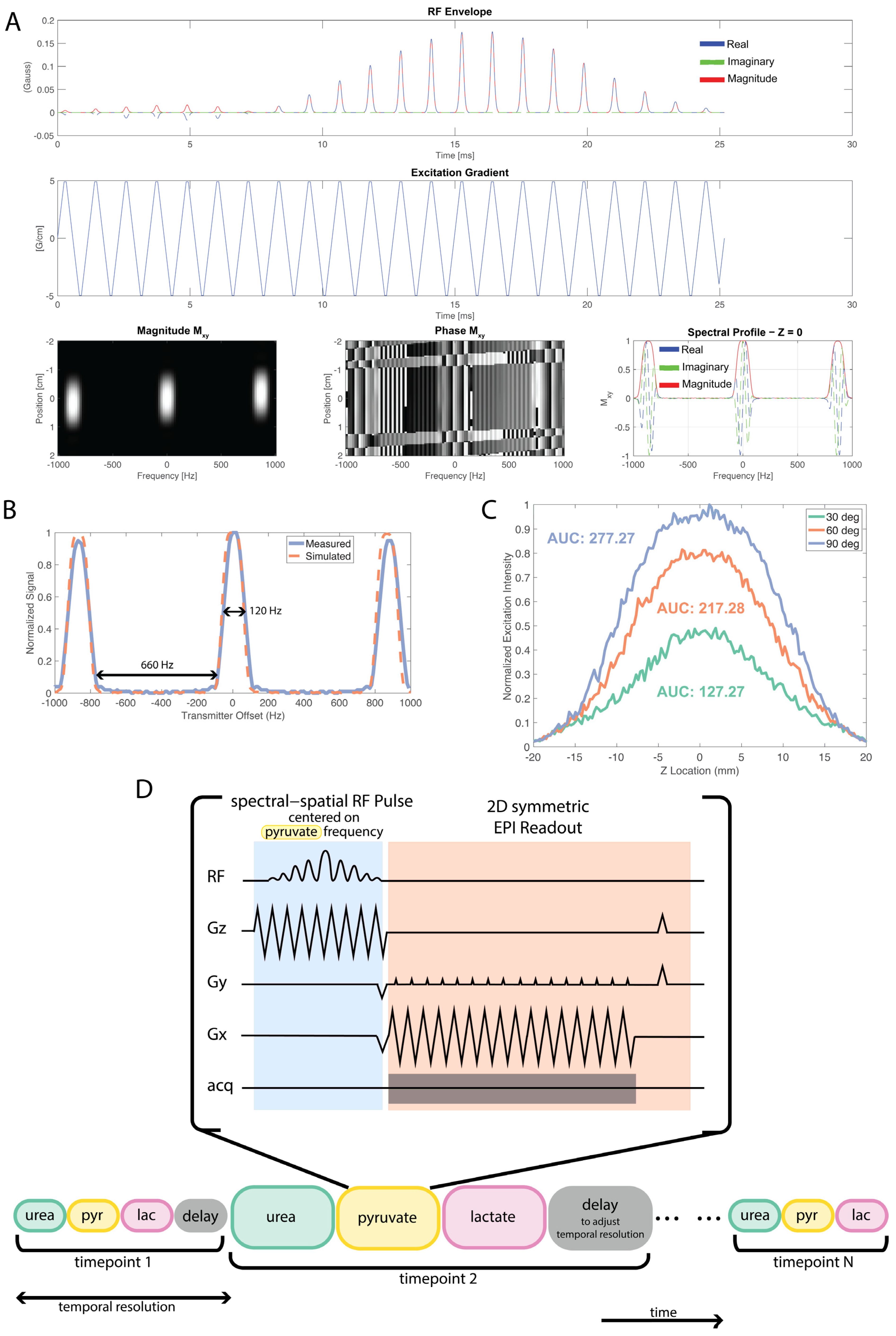
Abstract
:1. Introduction
2. Materials and Methods
3. Results
3.1. Spectral–Spatial Pulse Design and Calibration
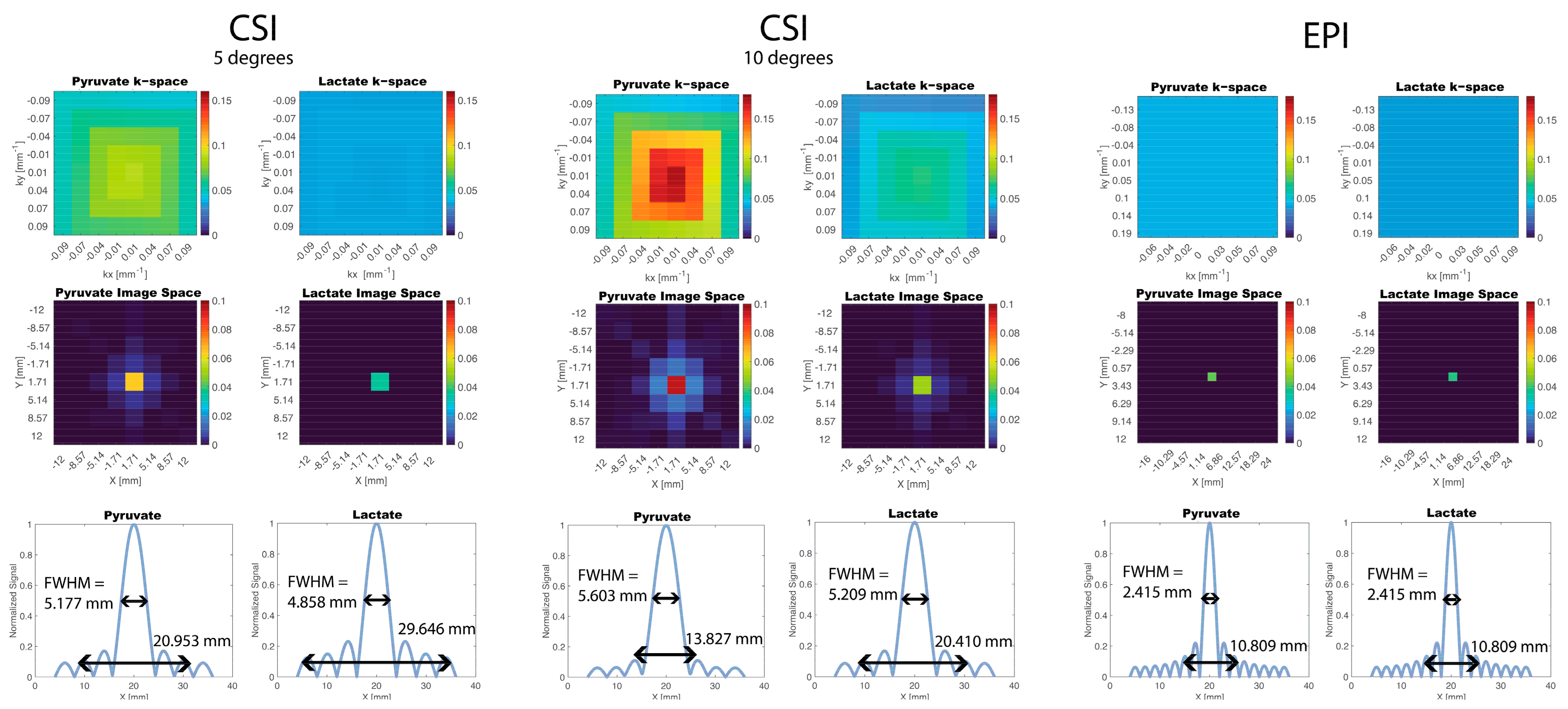
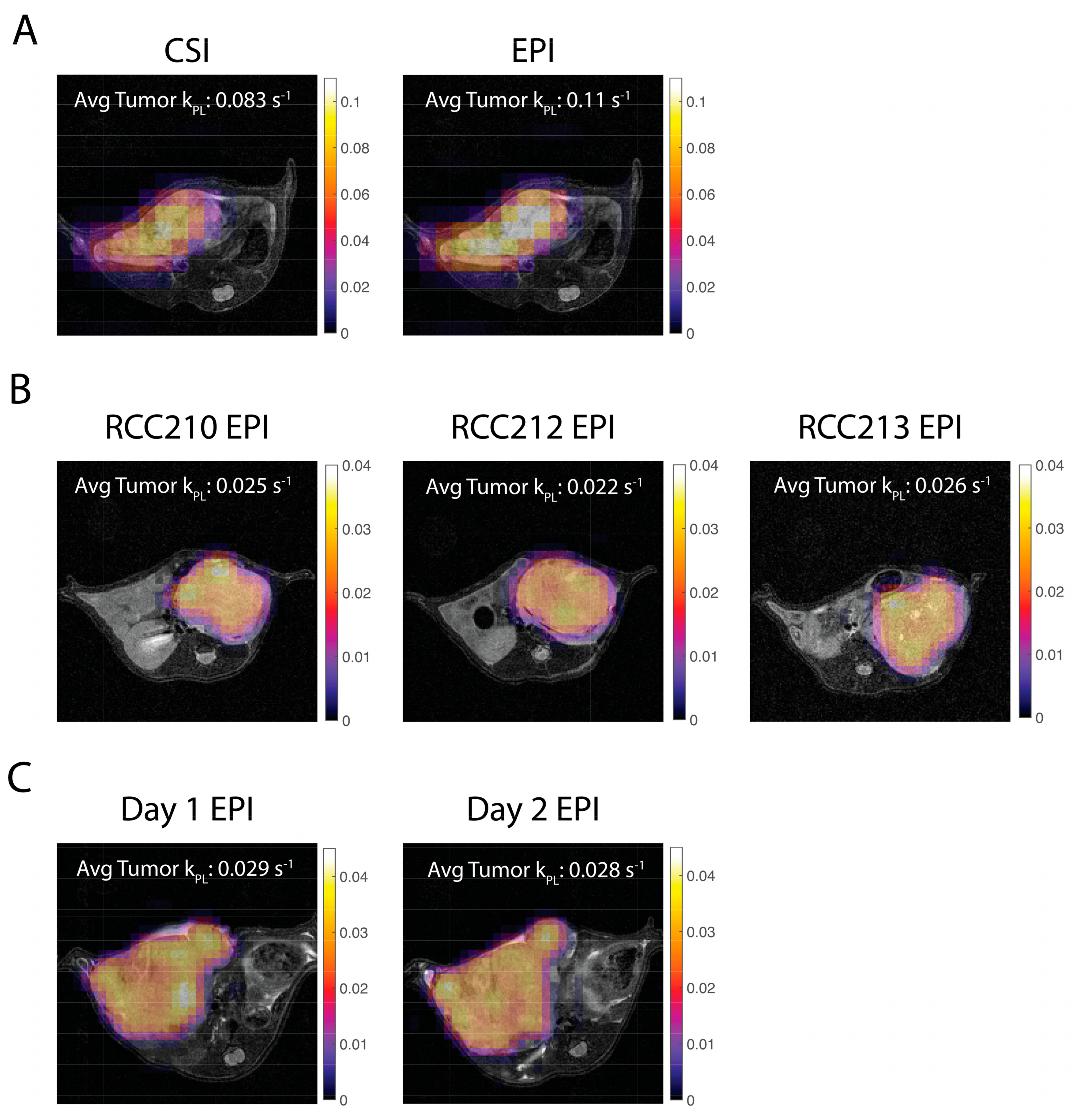
3.2. Comparison of EPI and CSI
3.2.1. Simulations
3.2.2. In Vivo Experiments
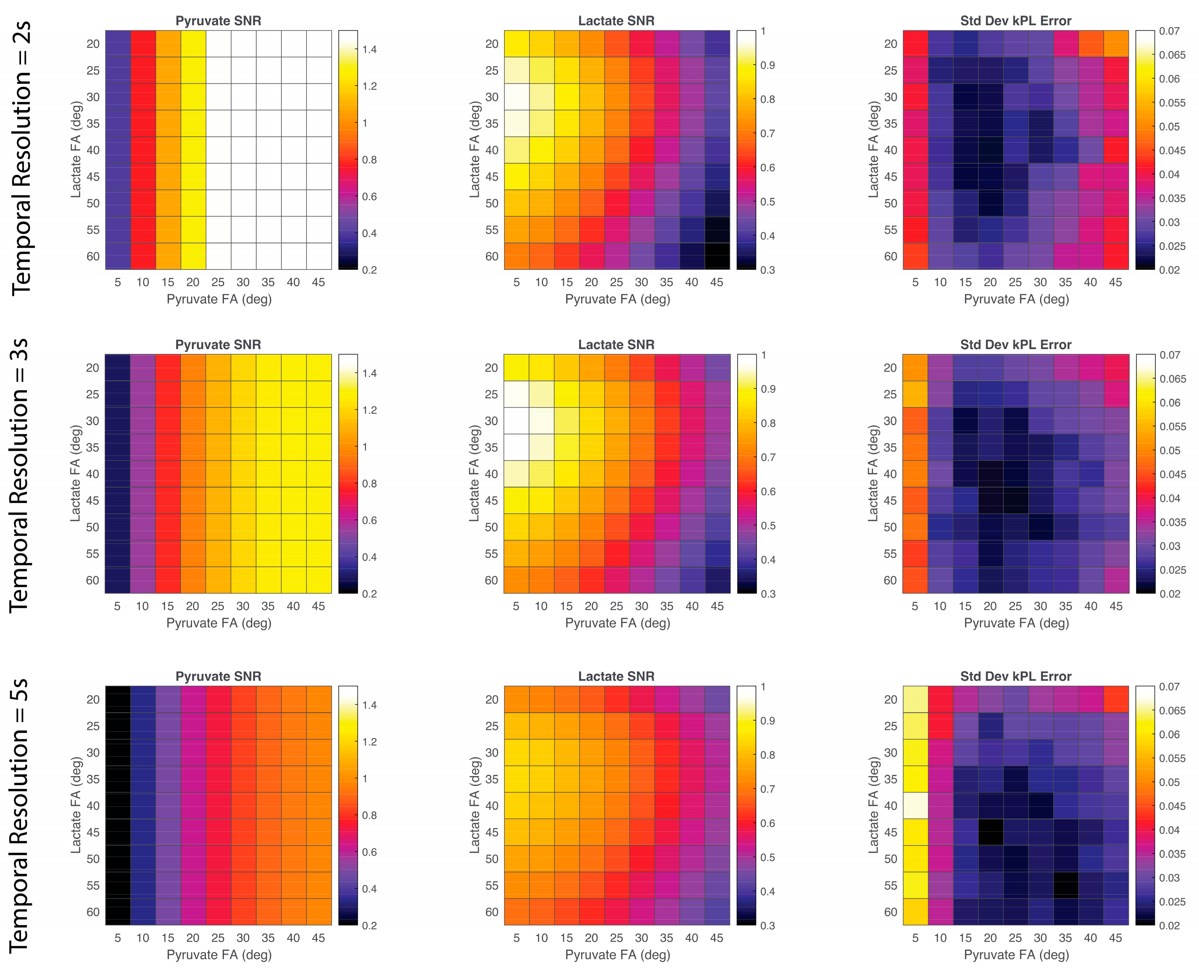
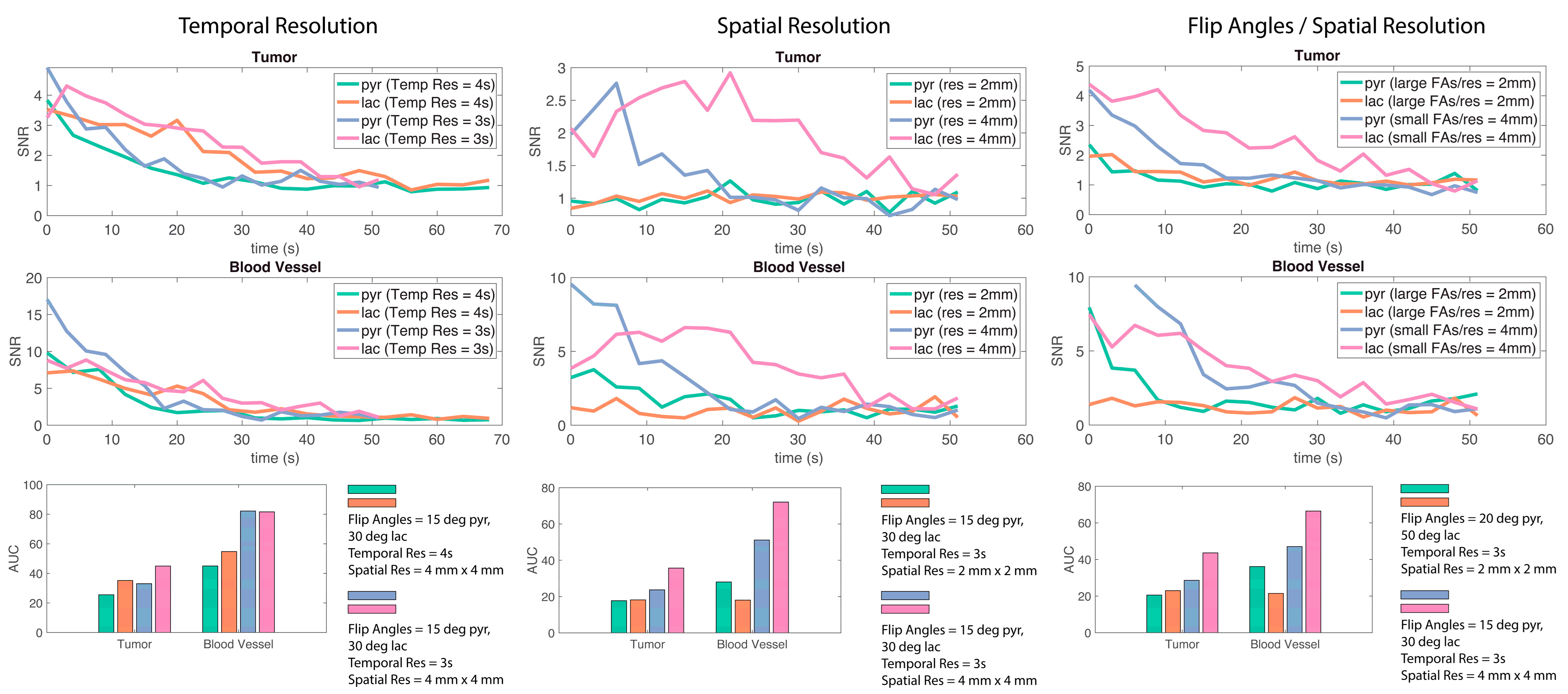
3.3. Testing In Vivo EPI Parameters Optimization for Robust SNR and kPL
3.3.1. Simulations
3.3.2. In Vivo Experiments
4. Discussion
4.1. Spectral–Spatial Pulse
4.2. CSI vs. spspEPI
4.3. Optimization of EPI Parameters
4.4. Pharmacokinetic Modelling and Quantification
5. Conclusions
Supplementary Materials
Author Contributions
Funding
Institutional Review Board Statement
Data Availability Statement
Conflicts of Interest
References
- Nelson, S.; Kurhanewicz, J.; Vigneron, D.; Larson, P.; Harzstark, A.; Ferrone, M.; Van Criekinge, M.; Chang, J.; Bok, R.; Park, I.; et al. Metabolic Imaging of Patients with Prostate Cancer Using Hyperpolarized [1-13C]Pyruvate. Sci. Transl. Med. 2013, 5, 198ra108. [Google Scholar] [CrossRef] [PubMed] [Green Version]
- Miloushev, V.Z.; Granlund, K.L.; Boltyanskiy, R.; Lyashchenko, S.K.; DeAngelis, L.M.; Mellinghoff, I.K.; Brennan, C.W.; Tabar, V.; Yang, T.J.; Holodny, A.I.; et al. Metabolic Imaging of the Human Brain with Hyperpolarized 13C Pyruvate Demonstrates 13C Lactate Production in Brain Tumor Patients. Cancer Res. 2018, 78, 3755–3760. [Google Scholar] [CrossRef] [PubMed] [Green Version]
- Gallagher, F.A.; Woitek, R.; McLean, M.A.; Gill, A.B.; Manzano Garcia, R.; Provenzano, E.; Riemer, F.; Kaggie, J.; Chhabra, A.; Ursprung, S.; et al. Imaging Breast Cancer Using Hyperpolarized Carbon-13 MRI. Proc. Natl. Acad. Sci. USA 2020, 117, 2092–2098. [Google Scholar] [CrossRef] [PubMed] [Green Version]
- Tang, S.; Meng, M.V.; Slater, J.B.; Gordon, J.W.; Vigneron, D.B.; Stohr, B.A.; Larson, P.E.Z.; Wang, Z.J. Metabolic Imaging with Hyperpolarized 13C Pyruvate Magnetic Resonance Imaging in Patients with Renal Tumors—Initial Experience. Cancer 2021, 127, 2693–2704. [Google Scholar] [CrossRef]
- Rider, O.J.; Apps, A.; Miller, J.J.J.J.; Lau, J.Y.C.; Lewis, A.J.M.; Peterzan, M.A.; Dodd, M.S.; Lau, A.Z.; Trumper, C.; Gallagher, F.A.; et al. Noninvasive In Vivo Assessment of Cardiac Metabolism in the Healthy and Diabetic Human Heart Using Hyperpolarized 13C MRI. Circ. Res. 2020, 126, 725–736. [Google Scholar] [CrossRef] [Green Version]
- Wang, Z.J.; Ohliger, M.A.; Larson, P.E.Z.; Gordon, J.W.; Bok, R.A.; Slater, J.; Villanueva-Meyer, J.E.; Hess, C.P.; Kurhanewicz, J.; Vigneron, D.B. Hyperpolarized 13C MRI: State of the Art and Future Directions. Radiology 2019, 291, 273–284. [Google Scholar] [CrossRef]
- Gordon, J.W.; Chen, H.; Autry, A.; Park, I.; Van Criekinge, M.; Mammoli, D.; Milshteyn, E.; Bok, R.; Xu, D.; Li, Y.; et al. Translation of Carbon-13 EPI for Hyperpolarized MR Molecular Imaging of Prostate and Brain Cancer Patients. Magn. Reson. Med. 2018, 81, 2702–2709. [Google Scholar] [CrossRef]
- Gordon, J.W.; Chen, H.-Y.; Dwork, N.; Tang, S.; Larson, P.E.Z. Fast Imaging for Hyperpolarized MR Metabolic Imaging. J. Magn. Reson. Imaging 2021, 53, 686–702. [Google Scholar] [CrossRef]
- Cunningham, C.H.; Chen, A.P.; Lustig, M.; Hargreaves, B.A.; Lupo, J.; Xu, D.; Kurhanewicz, J.; Hurd, R.E.; Pauly, J.M.; Nelson, S.J.; et al. Pulse Sequence for Dynamic Volumetric Imaging of Hyperpolarized Metabolic Products. J. Magn. Reson. 2008, 193, 139–146. [Google Scholar] [CrossRef] [Green Version]
- Shang, H.; Sukumar, S.; von Morze, C.; Bok, R.A.; Marco-Rius, I.; Kerr, A.; Reed, G.D.; Milshteyn, E.; Ohliger, M.A.; Kurhanewicz, J.; et al. Spectrally Selective 3D Dynamic Balanced SSFP for Hyperpolarized C-13 Metabolic Imaging with Spectrally Selective RF Pulses. Magn. Reson. Med. 2017, 78, 963–975. [Google Scholar] [CrossRef]
- Milshteyn, E.; von Morze, C.; Gordon, J.W.; Zhu, Z.; Larson, P.E.Z.; Vigneron, D.B. High Spatiotemporal Resolution BSSFP Imaging of Hyperpolarized [1-13C]Pyruvate and [1-13C]Lactate with Spectral Suppression of Alanine and Pyruvate-Hydrate. Magn. Reson. Med. 2018, 80, 1048–1060. [Google Scholar] [CrossRef] [PubMed]
- Lee, P.M.; Chen, H.-Y.; Gordon, J.W.; Wang, Z.J.; Bok, R.; Hashoian, R.; Kim, Y.; Liu, X.; Nickles, T.; Cheung, K.; et al. Whole-Abdomen Metabolic Imaging of Healthy Volunteers Using Hyperpolarized [1-13C]Pyruvate MRI. J. Magn. Reson. Imaging 2022, 56, 1792–1806. [Google Scholar] [CrossRef] [PubMed]
- Walker, C.M.; Fuentes, D.; Larson, P.E.Z.; Kundra, V.; Vigneron, D.B.; Bankson, J.A. Effects of Excitation Angle Strategy on Quantitative Analysis of Hyperpolarized Pyruvate. Magn. Reson. Med. 2019, 81, 3754–3762. [Google Scholar] [CrossRef] [PubMed]
- Tang, S.; Milshteyn, E.; Reed, G.; Gordon, J.; Bok, R.; Zhu, X.; Zhu, Z.; Vigneron, D.B.; Larson, P.E.Z. A Regional Bolus Tracking and Real-Time B1 Calibration Method for Hyperpolarized 13C MRI. Magn. Reson. Med. 2019, 81, 839–851. [Google Scholar] [CrossRef]
- Yen, Y.-F.; Kohler, S.J.; Chen, A.P.; Tropp, J.; Bok, R.; Wolber, J.; Albers, M.J.; Gram, K.A.; Zierhut, M.L.; Park, I.; et al. Imaging Considerations for in Vivo 13C Metabolic Mapping Using Hyperpolarized 13C-Pyruvate. Magn. Reson. Med. 2009, 62, 1–10. [Google Scholar] [CrossRef] [Green Version]
- Michel, K.A.; Ragavan, M.; Walker, C.M.; Merritt, M.E.; Lai, S.Y.; Bankson, J.A. Comparison of Selective Excitation and Multi-Echo Chemical Shift Encoding for Imaging of Hyperpolarized [1-13C]Pyruvate. J. Magn. Reson. 2021, 325, 106927. [Google Scholar] [CrossRef]
- Blazey, T.; Reed, G.D.; Garbow, J.R.; von Morze, C. Metabolite-Specific Echo-Planar Imaging of Hyperpolarized [1-13C]Pyruvate at 4.7 T. Tomography 2021, 7, 466–476. [Google Scholar] [CrossRef]
- Larson, P.E.Z.; Chen, H.Y.; Gordon, J.W.; Korn, N.; Maidens, J.; Arcak, M.; Tang, S.; Criekinge, M.; Carvajal, L.; Mammoli, D.; et al. Investigation of Analysis Methods for Hyperpolarized 13C-Pyruvate Metabolic MRI in Prostate Cancer Patients. NMR Biomed. 2018, 31, e3997. [Google Scholar] [CrossRef] [PubMed]
- Qin, Q. Point Spread Functions of the T2 Decay in K-Space Trajectories with Long Echo Train. Magn. Reson. Imaging 2012, 30, 1134–1142. [Google Scholar] [CrossRef] [PubMed] [Green Version]
- Hyperpolarized-MRI-Toolbox. Available online: https://github.com/LarsonLab/hyperpolarized-mri-toolbox (accessed on 18 March 2023).
- Agarwal, S.; Bok, R.; Peehl, D.; Sriram, R. Protocol: Intrahepatic Implantation of Tumor Cells; University of California: San Francisco, CA, USA, 2021. [Google Scholar] [CrossRef]
- Agarwal, S.; Peehl, D.; Sriram, R. Protocol: Intratibial Implantation of Tumor Cells; University of California: San Francisco, CA, USA, 2021. [Google Scholar] [CrossRef]
- Agarwal, S.; Peehl, D.; Sriram, R. Protocol: Single Cell Digestion of Tumor Tissue; University of California: San Francisco, CA, USA, 2021. [Google Scholar] [CrossRef]
- Agudelo, J.P.; Upadhyay, D.; Zhang, D.; Zhao, H.; Nolley, R.; Sun, J.; Agarwal, S.; Bok, R.A.; Vigneron, D.B.; Brooks, J.D.; et al. Multiparametric Magnetic Resonance Imaging and Metabolic Characterization of Patient-Derived Xenograft Models of Clear Cell Renal Cell Carcinoma. Metabolites 2022, 12, 1117. [Google Scholar] [CrossRef]
- Crane, J.C.; Gordon, J.W.; Chen, H.-Y.; Autry, A.W.; Li, Y.; Olson, M.P.; Kurhanewicz, J.; Vigneron, D.B.; Larson, P.E.Z.; Xu, D. Hyperpolarized 13C MRI Data Acquisition and Analysis in Prostate and Brain at University of California, San Francisco. NMR Biomed. 2021, 34, e4280. [Google Scholar] [CrossRef] [PubMed]
- Khegai, O.; Schulte, R.F.; Janich, M.A.; Menzel, M.I.; Farrell, E.; Otto, A.M.; Ardenkjaer-Larsen, J.H.; Glaser, S.J.; Haase, A.; Schwaiger, M.; et al. Apparent Rate Constant Mapping Using Hyperpolarized [1–13C]Pyruvate. NMR Biomed. 2014, 27, 1256–1265. [Google Scholar] [CrossRef] [PubMed]
- Ahamed, F.; Van Criekinge, M.; Wang, Z.J.; Kurhanewicz, J.; Larson, P.; Sriram, R. Modeling Hyperpolarized Lactate Signal Dynamics in Cells, Patient-derived Tissue Slice Cultures and Murine Models. NMR Biomed. 2021, 34, e4467. [Google Scholar] [CrossRef] [PubMed]
- Larson, P.E.Z.; Kerr, A.B.; Chen, A.P.; Lustig, M.S.; Zierhut, M.L.; Hu, S.; Cunningham, C.H.; Pauly, J.M.; Kurhanewicz, J.; Vigneron, D.B. Multiband Excitation Pulses for Hyperpolarized 13C Dynamic Chemical-Shift Imaging. J. Magn. Reson. 2008, 194, 121–127. [Google Scholar] [CrossRef] [PubMed] [Green Version]
- Gordon, J.W.; Autry, A.W.; Tang, S.; Graham, J.Y.; Bok, R.A.; Zhu, X.; Villanueva-Meyer, J.E.; Li, Y.; Ohilger, M.A.; Abraham, M.R.; et al. A Variable Resolution Approach for Improved Acquisition of Hyperpolarized 13 C Metabolic MRI. Magn. Reson. Med. 2020, 84, 2943–2952. [Google Scholar] [CrossRef]


Disclaimer/Publisher’s Note: The statements, opinions and data contained in all publications are solely those of the individual author(s) and contributor(s) and not of MDPI and/or the editor(s). MDPI and/or the editor(s) disclaim responsibility for any injury to people or property resulting from any ideas, methods, instructions or products referred to in the content. |
© 2023 by the authors. Licensee MDPI, Basel, Switzerland. This article is an open access article distributed under the terms and conditions of the Creative Commons Attribution (CC BY) license (https://creativecommons.org/licenses/by/4.0/).
Share and Cite
Sahin, S.I.; Ji, X.; Agarwal, S.; Sinha, A.; Mali, I.; Gordon, J.W.; Mattingly, M.; Subramaniam, S.; Kurhanewicz, J.; Larson, P.E.Z.; et al. Metabolite-Specific Echo Planar Imaging for Preclinical Studies with Hyperpolarized 13C-Pyruvate MRI. Tomography 2023, 9, 736-749. https://doi.org/10.3390/tomography9020059
Sahin SI, Ji X, Agarwal S, Sinha A, Mali I, Gordon JW, Mattingly M, Subramaniam S, Kurhanewicz J, Larson PEZ, et al. Metabolite-Specific Echo Planar Imaging for Preclinical Studies with Hyperpolarized 13C-Pyruvate MRI. Tomography. 2023; 9(2):736-749. https://doi.org/10.3390/tomography9020059
Chicago/Turabian StyleSahin, Sule I., Xiao Ji, Shubhangi Agarwal, Avantika Sinha, Ivina Mali, Jeremy W. Gordon, Mark Mattingly, Sukumar Subramaniam, John Kurhanewicz, Peder E. Z. Larson, and et al. 2023. "Metabolite-Specific Echo Planar Imaging for Preclinical Studies with Hyperpolarized 13C-Pyruvate MRI" Tomography 9, no. 2: 736-749. https://doi.org/10.3390/tomography9020059