
A Crash Data Analysis through a Comparative Application of Regression and Neural Network Models

1
Architecture, Built Environment and Construction Engineering Department, Politecnico di Milano, 20133 Milan, Italy
2
CERM, Politecnico di Milano, 20133 Lecco, Italy
*
Author to whom correspondence should be addressed.
Safety 2023, 9(2), 20; https://doi.org/10.3390/safety9020020
Submission received: 17 February 2023
/
Revised: 24 March 2023
/
Accepted: 31 March 2023
/
Published: 1 April 2023
Abstract
:One way to reduce road crashes is to determine the main influential factors among a long list that are attributable to driver behavior, environmental conditions, vehicle features, road type, and traffic signs. Hence, selecting the best modelling tool for extracting the relations between crash factors and their outcomes is a crucial task. To analyze the road crash data of Milan City, Italy, gathered between 2014–2017, this study used artificial neural networks (ANNs), generalized linear mixed-effects (GLME), multinomial regression (MNR), and general nonlinear regression (NLM), as the modelling tools. The data set contained 35,182 records of road crashes with injuries or fatalities. The findings showed that unbalanced and incomplete data sets had an impact on outcome performance, and data treatment methods could help overcome this problem. Age and gender were the most influential recurrent factors in crashes. Additionally, ANNs demonstrated a superior capability to approximate complicated relationships between an input and output better than the other regression models. However, they cannot provide an analytical formulation, but can be used as a baseline for other regression models. Due to this, GLME and MNR were utilized to gather information regarding the analytical framework of the model, that aimed to construct a particular NLM.
1. Introduction
According to the World Health Organization (WHO), road traffic crashes cause approximately 1.35 million fatalities worldwide each year, leaving between 20 and 50 million people with non-fatal injuries (WHO, 2022) [1]. The WHO reported that road traffic crashes have multi-factorial causes, including human factors, roads and other infrastructure factors, insufficient policing, environmental factors, and vehicle characteristics. Road users are reportedly the main cause of crashes. According to estimates, road traffic injuries are the eighth leading cause of death worldwide for all age groups and the leading cause of death for children and young people aged 5–29 years (WHO, 2018) [1].
Therefore, determining the most influential factors could help in taking appropriate actions to reduce the risk of road crashes. Further studies on these factors can be found in Williams and Carsten (2018), Hu et al. (1993); Massie et al., (1997) [2,3,4] for driver characteristics; in Bergel-Hayat et al. (2013); Brodsky and Hakkert (1988) [5,6] for environment; in Ulfarson and Mannering (2004) [7] for vehicle characteristics; in Noland and Oh, (2004) [8] for infrastructure; and in Abdulhafedh (2017) [9] for crash data collection methods.
Another task is to create an appropriate crash data set for potential modelling tools. Obtaining proper results and reliable models depends on the availability of a high-quality data set, representing precise information about potential affecting factors.
Some previous studies, for example Amoros et al. (2006), Abay (2015), and Watson et al. (2015) [10,11,12], stated that using police-reported crash data only results in misleading and incomplete inferences on road crash outcomes. However, Imprialou et al. (2019) [13] suggested that, to eliminate potential mistakes, the ultimate goal of the road safety research community should be to develop a seamless crash database, where all components can be integrated automatically. In addition, the sensitivity of the modelling tools to an unbalanced data set in terms of the response variable categories may affect the outcomes. Another objective outlined in recent literature is to predict crash risk in real time or near real time in order to prevent them from happening (Mehdizadeh et al., 2020; Dimitrijevic et al., 2022) [14,15].
One of the most important aspects of road crash analysis is the selection of the proper tool for modelling. Previous research methods and techniques (Fausett, 1994; Mccullagh and Nelder, 1985; Hosmer et al., 1989) [16,17,18] have been used to model crash data based on various approaches, such as crash severity and crash type. In this study, four different modelling tools, namely, artificial neural networks (ANNs) (Fausett, 1994) [16], generalized linear mixed effects (GLME) (Molenberghs et al., 2002) [19], a general nonlinear model (NLM) (Mccullagh and Nelder, 1985) [17], and a multinomial regression model (MNR) (Hosmer et al., 1989) [18], were chosen as the modelling tools for this study in order to meet the predetermined objectives.
Recently, papers such as Dimitrijevic et al. (2022) [15] presented several crash risk and injury severity assessment models in order to compare their performance: random effects, Bayesian logistics regression, Gaussian naïve Bayes, k-nearest neighbor, random forest, and gradient boosting machine methods have been trained and tested for this purpose. Iranitalaba and Khattakb (2017) [20] compared the performance of four statistical and machine learning methods, including multinomial logit (MNL), nearest neighbor classification (NNC), support vector machines (SVM), and random forests (RF), in predicting traffic crash severity. Vector quantization was used in Mussone and Kim (2010) [21] to cluster crash data through a self-organizing map.
The different performance and functionalities of modelling options make the choice of proper alternatives more difficult. Another difficulty in the choice is the functioning of the modelling tools. Distinctions in modelling tools have an effect when comparing their functionalities.
Moreover, ANNs are a robust tool for investigating complex phenomena without assuming any preliminary hypotheses about the model. Nevertheless, they do not provide an analytical formula in terms of their mathematical functions. Thus, only a sensitivity analysis can be performed to determine how explanatory variables affect outcomes. GLME and NLM models require an analytical formulation of the input–output relationship. Hence, the actual effect of the significant independent variables on the results can be calculated. MNR models have a predefined modelling structure and are used to compare and assess the results with those obtained by ANNs.
In addition, in the field of road safety, survey research is frequently used to study traffic behavior and its underlying cognitive and motivational determinants (Goldenbeld and de Craen 2013) [22]. To understand the factors influencing road crashes, constructing a questionnaire could provide knowledge of road users’ habits, perceptions, and beliefs. The road safety perception questionnaire should consider the singularities of the variables that cause road crashes (Espinoza-Molina et al., 2021) [23]. This study is multifaceted and focuses on three aims:
- To study crash data collected between 2014 and 2017 through a comparison of modelling methodologies, in terms of their performance and results, using four paradigms, namely, artificial neural networks (ANNs), generalized linear mixed-effects (GLME), multinomial regression (MNR), and general nonlinear regression (NLM);
- To find the analytical formulation that better describes the relationship between input and output;
- To analyze common variables of the models.
The data set contained 35,182 crash-related records. The primary differentiation between the modelling tools is their categorization. ANNs are machine learning tools. However, GLME, MNR, and NLM are related to regression modelling. The distinction between the modelling categorization is based on their functionalities, but similarities are being investigated.
The rest of this paper is organized as follows: Section 2 describes the methodology adopted in the research. Section 3 provides the information about the data set, such as explanatory and response variables and the preprocessing of data. Section 4 presents the modeling approaches used in this study. Section 5 describes the evaluation methods for modeling and then compares the outcomes. Finally, Section 6 discusses the outcomes and draws the conclusions of the study.
2. Methodology
The methodology adopted in the research includes the following steps:
- Analysis of data;
- Pre-processing and normalization of data;
- Model building;
- Check of model performance (if not satisfactory, we went back to step 3 for model building);
- Analysis of results and discussion.
Steps 3 and 4 were reiterated until performance was considered satisfactory or could not be further improved. This loop holds for all four models and only the MNR model required a few iterations to reach the final configuration. This methodological structure explains why model performance is presented just after the theoretical description of the models.
3. The Data Set
3.1. Database Information
The crash data used in this study come from the Lombardy Region in Italy, an institutional subject that collects information on crashes that result in injuries or fatalities occurring in the region. These data are the same as those managed by the Italian National Institute of Statistics.
The definition of injured people and the distinction between serious and minor injuries is made on the basis of AIS scale (AAAM, 2022) [24] which was adopted by the Italian Institute of Statistics in accordance with the European Commission directive.
The data refer to crashes that occurred in the city of Milan between 2014 and 2017. Each of them has been considered an independent observation with different characteristics. There are 35,182 records described by 16 explanatory variables, 14 of which are used as independent variables and 2 as distinct dependent variables:
- Crash type, with three categories, including between circulating vehicles, pedestrian hit, and isolated vehicle crash;
- Crash effects, with two categories, including injuries and fatalities.
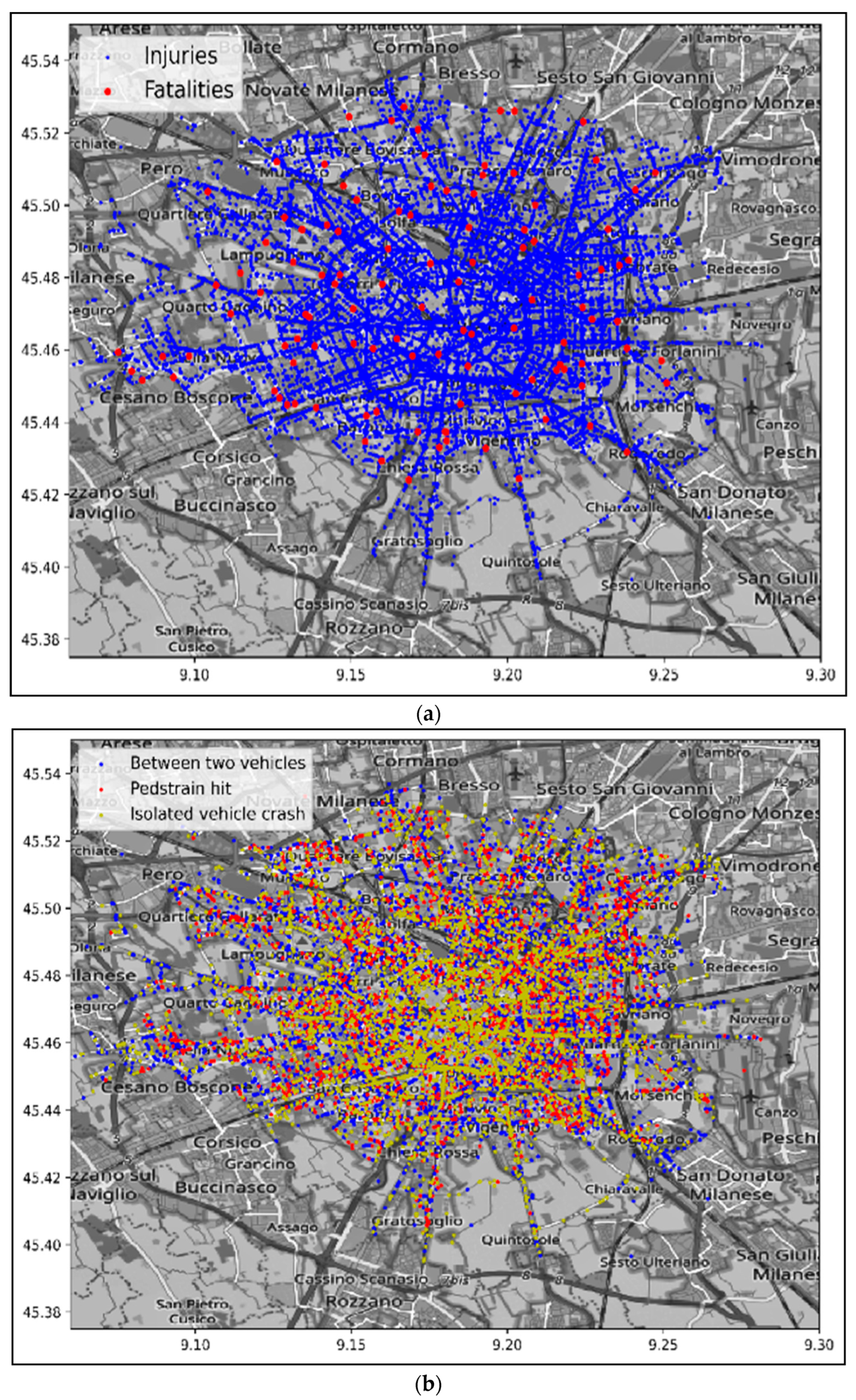
Owing to their geo-referenced localization, the distribution of crashes by severity and type of crash in Milan City is presented in Figure 1a,b. In the figures, the density of crashes with an injury outcome is significantly higher than that of fatal crashes. Meanwhile, the categories of crash types are subdivided more homogenously among types and on the territory of the city. Only the first two vehicles (vehicles A and B) involved in a crash were considered in the research.
3.2. Data Set Variables
Fourteen explanatory variables were chosen among the different possible variables available in the original data set. The following is the set of variable types (see Table 1 for the details and the basic statistical information):
- Variables referring to the road conditions;
- Variable referring to the infrastructure;
- Variables referring to the crash characteristics;
- Variables for vehicle characteristics;
- Variables for driver’s description.
Two variables are chosen as output variables:
- 6.1.
- Crash effects, indicating the severity of the crash;
- 6.2.
- Type of crash, indicating the dynamic of the crash.
The distributions of the observations between the categories of the variables are presented in Table 1.
Unfortunately, no data about the socio-economic characteristics of the people involved in the crashes are available and, due to anonymity of data, they cannot be subsequently retrieved.
3.3. Data Oversampling and Normalization
One of the issues that can affect modelling is related to an imbalanced data set. As presented in Table 1, a noticeable difference exists between the frequencies of the two categories of output C15 (but not so critical for C16); this affects machine learning performance and generally all other (though nonlinear) regression models. For example, categories with a low number of counts in the training set are almost always ignored by artificial neural networks, and this affects model performance (references to these models can be found in the section Models and Their Performance). Different solutions have been suggested in previous studies to address this issue. Two methods are proposed in the literature: under-sampling and over-sampling. Under-sampling methods are generally used in conjunction with an over-sampling technique for the minority class, and this combination often results in better performance than using over-sampling or under-sampling alone on the training data set. The major drawback of under-sampling is that this method can discard potentially useful data that could be important for the induction process. This holds particularly for crash data that suffer on their own because of the high dishomogeneity of possible combinations of data.
Ling et al. (1998) [25] proposed a method in which a category with a low count in the data set was over-sampled to match the size of other classes. According to their study, we decided to use over-sampling and not under-sampling in order to lose no data information for both majority and minority classes. A simple duplication of the minority class in output C15 was carried out to achieve the similar number of observations as in the other class (leading to a data set size of 70087 records).
Another issue is related to the different scales between variables, which may also cause training distortions. To solve this issue, all numerical inputs were normalized in the range from 0 to 1, using the formula in Equation (1) (Dutka, 1988) [26]:
where Xnorm is the normalized value of variable X and Xmax and Xmin are the maximum and minimum values of X, respectively. Binomial variables do not require normalization, while categorical variables are coded in a binary base (e.g., 6 is coded as “110” by using three independent inputs).
4. Models and Their Performance
4.1. Back Propagation Artificial Neural Network
Some previous studies, such as Mussone et al. (1999), Chakraborty et al. (2019), Ali and Tafour (2012), Mussone et al. (2017), and Huang et al. (2016) [27,28,29,30,31], focused on the application of NNs on crash data sets and demonstrated their power in predicting the proper outcomes. A back propagation artificial neural network is a particular NN that computes the input function by propagating the input neuron’s computed values to the output neuron(s) using the weights of links connecting neurons as intermediate parameters. Learning occurs by iteratively changing those weights over many input–output pairs to ensure that more accurate predictions can be provided.
As we decided to study the two dependent variables separately to make the interpretation of outcomes easier, we developed two distinct NN structures. The training procedure was identical for both models, First, the data set was divided randomly into three different sets: training, testing, and validation sets with 60%, 20%, and 20% of the data, respectively.
The training data set was used during the training process to calculate the weights for links in the NN layers. At each iteration, the test set is used to calculate the network performance and decide to stop learning. Then, the validation set tests the model with data that has never been seen before and calculates the actual NN performance. The procedure was repeated a number of times to check whether data dishomogeneity affected the outcomes.
The disadvantage of using the back propagation artificial neural network (BPNN) approach is that the NN model is a black box, and the relationships between variables are not deducible from the inspection of weights.
Therefore, no analytical formulation between the input and output can be obtained directly. The effects of the input variables were analyzed through a sensitivity analysis of the model. Performance was evaluated according to mean squared errors (MSE) (Equation (2)), where n = number of data points, Yi = observed values, and Y’i = predicted values:
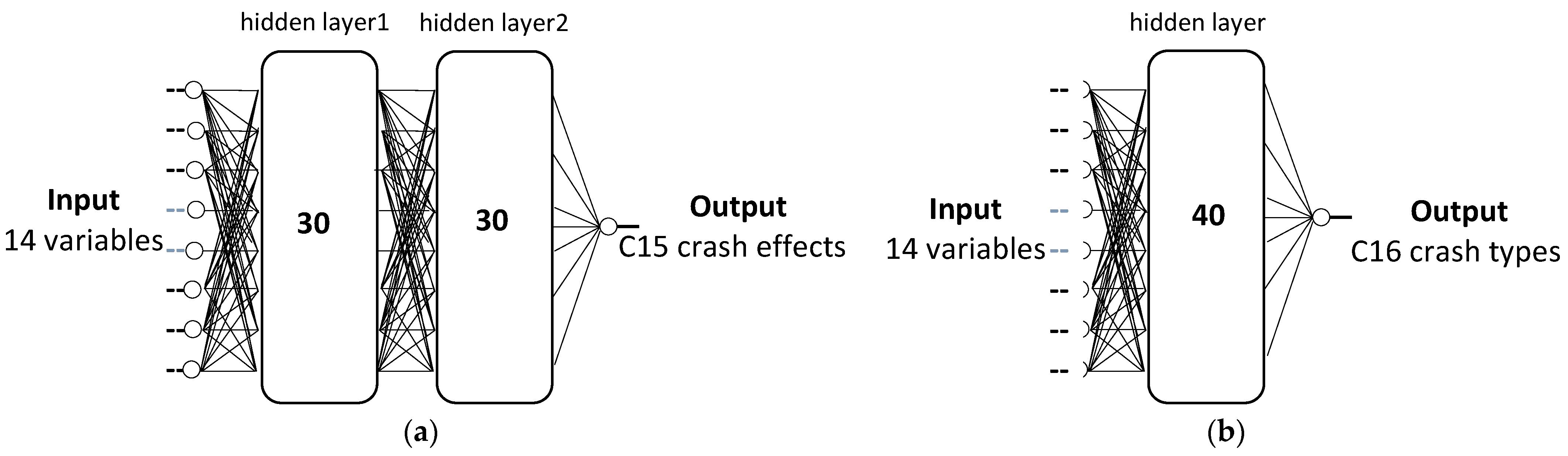
The BPNN is trained by updating the weight and bias values according to the Levenberg–Marquardt optimization algorithm (Kumaraswamy, 2021) [32]. The model was constructed using an input layer containing the 14 independent variables (C1–C14) reported in Table 1, hidden layers, and an output layer, with only one output corresponding to the C15 or C16 variables. As explained in the previous section, all categorical variables were coded in a binary format to reduce the connection between their values.
The data set was divided into three subsets according to the following percentages: 60%, 20%, and 20% for train, test, and validation sets, respectively. This configuration was the outcome of many trials focused on optimizing performance. The tuning of internal parameters was made by using an interface program which optimized them based on the performance achieved by using the validation set (such as internal weights). The Levenberg–Marquardt algorithm adaptively varies the parameter updates between the gradient descent and the Gauss–Newton update. Overfitting is controlled by the test and validation sets. To increase the reliability of the models, we repeated the division of the data set into the three training subsets more times and checked if outcomes were similar or affected by the subset composition. The final structure of ANN is, in turn, the result of many trials with a different number of hidden layers and hidden neurons. This is an empirical activity. The best structures for response variables were created with two hidden layers with 30 neurons each for C15 (Figure 2a) and one hidden layer with 40 neurons for C16 (Figure 2b).
The networks had an MSE of 0.018 for the C15 and 0.049 for the C16 models. The MSE for C15 implies that there are approximately two errors for each of the one hundred samples, because the maximum error for this case is one. For output C16, the errors may assume different values (because the output varies from one to three). However, considering the confusion matrix of this model (in the Appendix A, Table A1), it can be deduced that there are approximately five errors for every one hundred samples. It is worth noting that MSE (or equivalently the RMSE) is generally used for NN training though in some cases it may give classification problems that, fortunately, were not experimented for these models. In any case, the comparisons between other regressive models were made by considering all the calculated indices.
4.2. Generalized Linear Mixed Effects (GLME)
For the analysis of multilevel data, random clusters and/or subject effects should be included in the regression model to account for the data correlation (Mussone et al., 2017) [30]. Generalized linear models (GLMs) extend classical linear models by allowing responses to follow distributions in the exponential family and allowing nonlinear relationships between the response and covariates. The exponential family includes a wide range of commonly used distributions, such as normal, binomial, and Poisson distributions (Wu, 2010) [33]. Fixed- and random-effect terms are the main components of generalized linear mixed effects (GLME) (Molenberghs et al., 2002) [19]. Fixed-effect terms are the conventional linear regression parts of the model, while random-effect terms are associated with individual experimental units drawn at random from a population and account for variations between groups that might affect the response. Random effects have prior distributions, whereas fixed effects do not. The general formulation and standard forms of the GLME model (Molenberghs et al., 2002) [19] are expressed as follows:
Here, yi is the outcome variable, Distr is a specified conditional distribution of y given b, μ is the conditional mean of yi given bi and μi is its ith element, σ2 is the dispersion parameter, w is the effective observation weight vector, g(μ) is a link function, X is a matrix of the predictor variables, β is a column vector of the fixed-effect regression coefficients, Z plays the role of design matrix for the random effects, b is a vector of the random effects, and ε is a column vector of the residuals.
In this study, the “log” (Equation (7)) link function has been used because a Poisson or binomial distribution is assumed for the output variables. Finally, the model for the mean response μ can be written as in Equation (8), where g−1 is the inverse of the link function g(μ) and η is the linear predictor of the fixed and random effects of the GLME:
As modelling with the original data set by using GLME ignores the prediction of correct values for the fatality case crashes, an oversampled data set was also used for the response variable C15. It is worth noting that GLME models do not require independence from the observations. The log link function and a binomial distribution as a probability mass function were employed.
The best performance was calculated by minimizing the log-likelihood index; other indexes (i.e., Akaike’s information criterion, AIC; Bayesian information criteria, BIC) were also estimated to control for the minimization process. For the C16 model, because the responses of the trials were acceptable without oversampling the data set, the original data set was used. Therefore, according to the given formulations, after a more or less long series of trials with different combinations of independent variables, the GLME models that provide the best performance for C15 (Equation (9)) and C16 (Equation (10)) are formulated as follows using Wilkinson’s notation:
Here, Cx (x = 1, …, 14) are the independent variables, C2|C11 denotes that C2 is analyzed after grouping data by C11, and C42–C4 indicates that only second-order effects of C4 are considered.
Table 2 shows the statistical analysis results of the GLME model for C15, where all P values were lower than 0.001. The standard error of estimates (SE) is generally much lower than the estimates, and the lower and upper bounds of the confidence interval (CI) never include zero. The estimated coefficients reveal the positive contributions of C8, C9, C42, and C92. Thus, to better understand the effect of variables, marginal effects analysis was applied through the analytical GLME model by computing the change in output by a unitary increment of the considered variable. The same analysis was developed for C16, as presented in Table 3. The positive contribution of C5 and C9, in addition to the negative contributions of C4, C7, and C92, is evident in the model. Confusion matrices for C15 and C16 are in Table A2 and Table A6 in the Appendix A, respectively.
4.3. Multinomial Regression (MNR)
The MNR model is a classification model used to generalize the binomial logistic regression to multiclass problems; in other words, more than two possible discrete outcomes are available as response variables. The MNR model indicates the probability of observation i choosing outcome k given the observation’s measured characteristics. The outcome of a response variable can be a restricted set of possible values. Because no natural order exists among the response variable categories in the used data, the model’s chosen response mode is the nominal response. The mathematical representation of the model with four output categories can be written as the following systems of relationships (Equation (11)):
Here, Xn is an input variable, θj = P(y = j) is the probability of an outcome being in category j, k is the number of response categories, and n is the number of predictor variables. The last category was used as a reference variable, written as the kth category. Further, βjn are the coefficients in the model that realize the effects of the predictor variables on the log odds of being in category j versus the reference category k. The most important assumption is to set the kth category coefficients. Therefore, the probability of being in each category j is
Similar to other modelling methods, MNR could not predict the fatal crash category in the C15 model. Thus, an oversampled data set was applied. The α values in Table 4 and Table 5 represent the intercept values of the model. Because some of the p value calculations are greater than the threshold value, the related variables must be considered removed from the model.
Because the C16 output has three different categories, the nominal MNR model can be represented by two equations. The isolated vehicle crash category was selected as the model reference category, and the predicted values of the model depict the relative risk of being in one category versus being in the reference category. Therefore, the highest probability was selected as the predicted value for the model. The model’s statistical representations for the C16 output variable are presented in Table 5 (non-significant variables are highlighted by a grey background).
The statistical analysis reveals that the importance of driver B information emerges by comparing the values of the coefficients with each other. Because driver B information has positive coefficients, the probability of being in the first category against the reference category increases by increasing the components of driver B, such as C11 and C12. Meanwhile, an increase in the C7 input variable decreases the probability of being in the first category and increases that of being in the second category.
4.4. General Nonlinear Regression (NLM)
Nonlinear regression is a form of regression analysis in which observational data are modeled by a function that is a nonlinear combination of model parameters, completely determined in its form by the researcher, and depends on one or more independent variables. The data were fitted using successive approximations. These models can make better predictions for unobserved data than other models whose analytical form is limited.
A general representation of the parametric nonlinear regression model is shown in Equation (15):
where y is the representation of response variables, X is the vector of input variables, β is the vector of the unknown parameters to be estimated, ε is the vector of identically distributed random disturbances, and f is a function of X and β. The assumptions for a standard nonlinear regression model are as follows:
- Errors are independent;
- Errors have mean zero and constant variance;
- Errors are normally distributed.
Some of these assumptions may be relaxed for more general models. This type of model attempts to find a parameter β that minimizes the MSE between the observed responses y and the predictions of the model f(X,β). To accomplish this, a starting value β0 is required before iteratively modifying the vector β to a vector with a minimum MSE.
Similar to the case of GLME, the oversampled data set was used for the crash effect response values. After many trials for both models, the best NLM models for C15 and C16 were obtained by using the analytical combinations in Equations (16) and (17), respectively:
(β4 ∗ exp (β44 ∗ C4) + (β9 ∗ C9) + (β411 ∗ C4 ∗ C11) + (β5 ∗ C5) + (β6 ∗ C6) + (β7 ∗ C7) +
+(β711 ∗ C7 ∗ C11) + (β913 ∗ C9 ∗ C13) + (β12 ∗ C12) + (β13 ∗ C13)
+(β711 ∗ C7 ∗ C11) + (β913 ∗ C9 ∗ C13) + (β12 ∗ C12) + (β13 ∗ C13)
(β2 ∗ C2) + (β4 ∗ exp (β44∗C4)) + (β5 ∗ C5) + (β7 ∗ C72) + (β8 ∗ C8) + exp (β913 ∗ C9 ∗ C13) +
+ (exp (β99 ∗ C9) + exp (β11 ∗ C11))/(1 + β90 ∗ C9)
+ (exp (β99 ∗ C9) + exp (β11 ∗ C11))/(1 + β90 ∗ C9)
The p values of the coefficients of all the combinations are around zero, and then significant, for models C15 and C16.
Unlike the GLME model, the NLM model does not require a link function between the explanatory and response variables. Thus, the obtained coefficients represent the actual influence on the model. Table 6 shows that the road infrastructure type (C4) had the most significant effect on the C15 model. Statistical analysis for C16 (Table 7) showed that the most influential variable was C9 (gender B).
5. Analyses and Results
5.1. Database Information Content
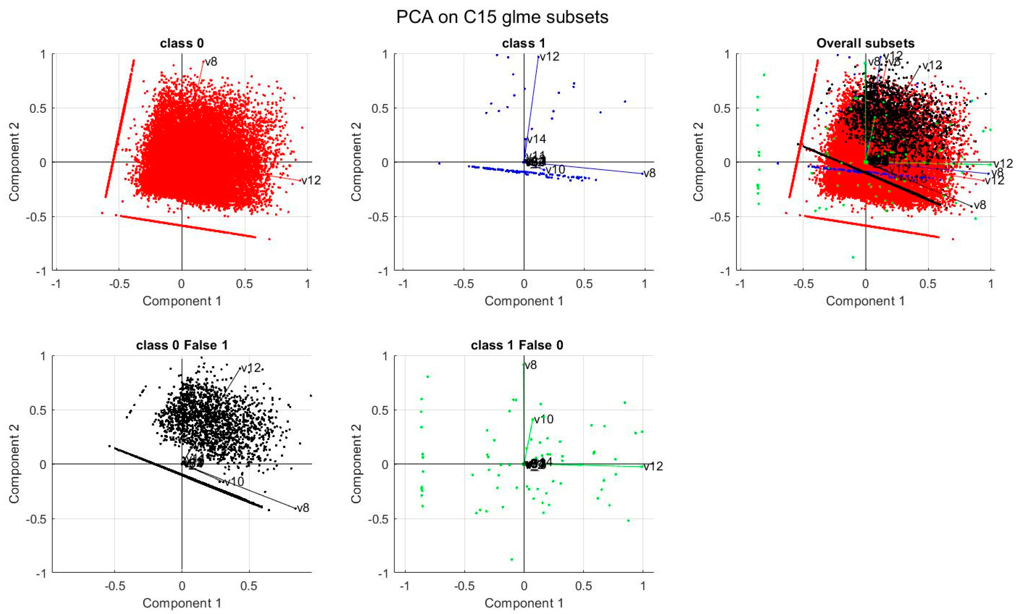
Principal component analysis (PCA) (Lebart et al., 1986) [34] was used to investigate the information content of the database and to identify the main variables explaining variance in the data. In this study, PCA was applied to understand why, for C15 models, only NN achieved good performance. Hence, we considered the four subsets of data according to the classification made by the GLME model (represented by the confusion matrix in Table A6): true injuries (class 0); false injuries (false 0); true fatalities (class 1); false fatalities (false 1). A PCA was carried out for each of them, and their outcomes are plotted in Figure 3.
The first four principal components explain more than 99% and the first two 86% of the overall variance; the related variables are C8, C10, C12, and C14 (age and years of driving license of drivers A and B, respectively). Considering that C10 and C14 are collinear with C8 and C12, we can assume that C8 and C12 are the actual crucial variables for modelling. It is worth noting that the mentioned variables are also related to the driver’s licensing age.
In Figure 3, true injuries (red) and false fatalities (black) almost overlap. The same, though to a lesser extent, occurs for true fatalities (blue) and false injuries (green). This accounts for the difficulties in increasing the performance of the GLME, NLM, and MNR models, which, contrary to NN, are not capable of such a discriminant property for those types of data.
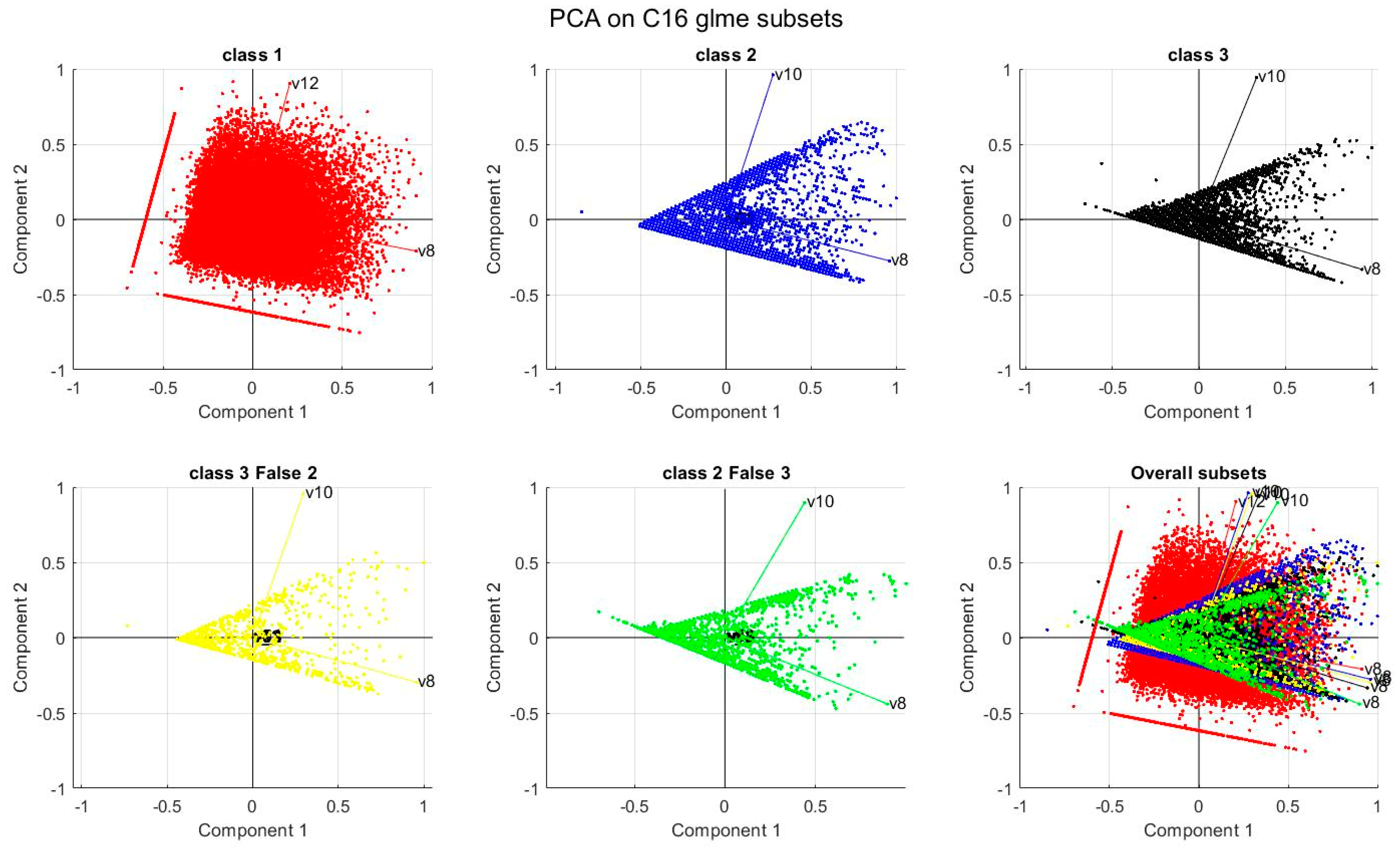
The PCA analysis for the C16 model was applied to five subsets of data corresponding to those calculated by using the GLME model (Table A6). For class 1 (crash between circulating vehicles), variance in data (red points) is well represented by variables C8 (i.e., age of driver A) and C12 (i.e., age of driver B). For the other two classes (2, pedestrian hits; 3, isolated vehicles), the situation is slightly confusing. For all four subsets, the two main principal components are represented by variables C8 and C10. As shown in Figure 4, the subsets for false cases (yellow and green points) are almost indistinguishable, as in the C15 model, but in this model, these bad samples are far fewer.
5.2. Sensitivity Analysis
Neural networks do not provide an analytical formulation between input and output variables. One way to address this issue is to conduct a sensitivity analysis. A sensitivity analysis is carried out by varying the input values individually or in a limited group (scenario) and by observing how the output varies. A number of scenarios were prepared from a large number of possible scenarios. These scenarios aim to consider some possible and typical crash situations involving male or female drivers during daytime or nighttime, with rainy weather or dry road surfaces, or with elderly drivers.
The main outcomes can be synthesized as follows: For the C15 model, a fatality crash is more likely to occur when driver A’s age is high. The difference between weather conditions in scenarios reveals that older drivers are prone to fatal crashes in unstable weather conditions. Conversely, the age of driver B does not significantly affect the output in most of the prepared scenarios. The time of crash and road conditions play a crucial role together with road typology. For example, if the road typology is a one-way carriageway in wet road conditions, a fatal crash can occur at night.
By applying sensitivity analysis to the C16 model, it was revealed that an increase in driver A’s age during unstable weather conditions (such as rainy weather with wet road conditions) significantly affected the output classified as the pedestrian hit crash type, regardless of the time of crash. However, younger drivers, such as driver B, were prone to having the same output. In addition, driver B’s licensing year variable is related to pedestrian hit crashes.
Another method to roughly assess the relative importance of input variables is to cancel one variable at a time and then calculate the new best NN and its performance. The variable whose cancelation leads to the worst performance is the most important. This method does not consider second order effects but is remarkable for its simplicity. When applied to the C15 and C16 models, it confirms and completes the outcomes of sensitivity analysis (as reported in Table 8).
5.3. Marginal Effects Analysis
Another method to analyze the effect of input when the analytical model is available, such as in GLME, is marginal effects analysis (MEA). MEA reveals the changes in a model’s response values when a specific input variable changes in a unit, while the other variables are assumed to be constant. Suppose the model is and C1 is the variable under consideration. Its marginal effect, ME, is
where y’ is the new value for the response variable after a unitary increase in the input variable, C1′ = C1 + 1. The higher the ME, the stronger the effect of the variable. If β > 0, ME > 1, and if β < 0, ME < 1. If the formula involving the variable is not linear, the calculations are more complex, but the procedure is identical. The outcomes of this analysis are reported in the synoptic Table 8.
5.4. Model Comparison
Finally, to compare the model’s performance, a confusion matrix is considered (Powers, 2020) [30]. A confusion matrix, also known as an error matrix, is a table where each column represents the instances in a predicted class (if the output is continuous, it can be divided into classes) and each row represents the actual class instances. Precision, also called positive predictive value, is the fraction of relevant instances among the retrieved instances. Meanwhile, recall, also known as sensitivity, is the fraction of retrieved relevant instances among all relevant instances. The “a-priori” rate (PR) (Equation (19)) corresponds to the percentage of the predicted crashes to the total to be predicted for each severity level, and the “a posteriori” rate (PO) (Equation (20)) is the percentage of predicted crashes to the total of predicted crashes for each severity level (Powers, 2020) [35].
where aij represents the number of predicted cases i and n is the matrix dimension.
Finally, the confusion matrix’s overall accuracy can be calculated using Equation (21) (Powers, 2020) [35]:
Accuracy is a more aggregate measure than PR and PO. The confusion matrices in Table A1, Table A2, Table A3, Table A4, Table A5, Table A6, Table A7 and Table A8 show the outcomes for the four model paradigms and for the two outputs: C15 and C16. In Table A1, the class “−1” is created by the ANN model in the recall mode; it may be that ANNs extrapolate output outside the interval used for training. As with other aggregated indices, accuracy is not a perfect measure of performance. In the case of the C15 model, its value is conditioned by the high level of imbalance in the data and by the oversampling procedure. In Table 8, a summary of model performance (accuracy, PR and PO by row and column, respectively) is reported.
The C15 output achieved the best performance (accuracy = 97.4%) in the ANN model, but not without any issues. First, a class with C15 = −1 is created, likely due to the ANN extrapolation function (which must be considered a negative capability because it is not controlled by actual data). Second, the “perfect” prediction of class 1 is attributable to oversampling; therefore, overtraining cannot be excluded. The confusion matrices for the other models were similar. Although an oversampled data set is also used, no definitive benefit is achieved and fatal crashes and those with injuries are still hardly discernible from each other (for the reasons reported by PCA in Section 4.1). For GLME and NLM models, the crucial point is to find the optimal relationship between the input variables, considering not only first- and second-order effects but also their interactions. Because the MNR model does not require an analytical formulation to model the data, it does not appear to be a suitable model when input data have complex relationships with the output.
For the C16 output, the ANN still achieved the best performance (accuracy is 93.4%), whereas the other models had similar outcomes (accuracy is never less than 91%). Differences between models are due to the different capabilities to distinguish between classes 2 and 3 (i.e., pedestrian hit and isolated vehicle crash) because class 1 is perfectly forecasted. The PCA in Section 4.1 explains the reason for this, and it may be that either further variables are needed, or events have a strong random component.
Table 8 presents the synoptic table of the model performance that synthesizes previous analyses. For the most part, the most relevant variables are age and gender of driver A and B and the type of road infrastructure (be it section or intersection). For output C15, road typology and meteorological conditions are also relevant; and for output C16, road conditions.
6. Discussion and Conclusions
The comparison of the performance of models for crash risk evaluation is a task developed by some authors (as in Iranitalaba and Khattakb (2017) [20] and Dimitrijevic et al. (2022) [15]. A common result between them and the present study is that model performance varies with the model type and with it also most significant variables (see Table 8 for a synoptic of used variables in the models developed in this research). A cross-comparison between results achieved with different data sets is not very feasible not least because of their differences; this is true not only for data distribution but also for the available fields present in the data sets themselves.
In the review paper by Slikboer et al. (2020) [36], twenty studies on the prediction of road crashes were taken into consideration, and among them only one reported an independent variable (driver gender) which was also used in our research. In the paper by Zhang et al. (2018) [37], road and meteorological conditions were the only significant fields to be compared.
A comparison of performance between different models is of certain interest; however, it must be considered that performance depends greatly on the contents of the data set (mainly related to the distribution of cases and the relationship between input and output). In the paper by Zhang et al. (2018) [37], the overall accuracy for six machine learning and statistical models ranges from 44% to 53.9%. Random forest behaves better, but no NNs are used.
In Iranitalaba and Khattakb (2017) [20], the best overall performance in predicting the costs of crashes is achieved by NNC (nearest neighbor classification) followed at a distance by SVM (support vector machine), RF (random forest), and MNL (multinomial logit).
Apart from these issues in comparing the different experiences on the subject, one limitation of this study is the contents of the data set; they do not include information about the socio-economic characteristics of people involved in the crashes, or about the flow when the crash occurred, or the speed of involved vehicles. Another limitation is that not all possible types of models have been investigated: only four. GLME and NLM models require an analytical formulation in advance. Unlike the ANN model, oversampling the data set did not improve their overall performance. However, because of the insertion of the analytical formulation, the actual effect of each input variable can be determined. Nevertheless, having many different ways of combining input variables makes analytical formulation a tricky exercise. Despite the expectations and the efforts, the performance of NLM did not overcome that of GLME and this proves that the knowledge about crash data contents is still incomplete. In addition, different analytical formulations may lead to models that appear different but have the same performance. In this contest, MNR presents a relatively higher ease of application but with no way to improve performance.
Another critical issue is the use of regression models in classification problems; this can hinder their application if the structure of output data is too complex (e.g., with more than one field).
Future studies should still focus on finding the optimal analytical formulation for regression models. In addition, research can be conducted to discover suitable data treatment methods for cases where the data set includes incomplete information or unbalanced data distribution. Notably, acquiring flow data as additional information for road crash analysis may positively affect the results of future studies. In addition, the current data set contains all crashes with injured people or fatalities. However, from a probabilistic measure of risk, there should also be a focus on crashes with only property damage, and there would be an interest in those events that did not lead to whatever type of crash for casualties.
Hence, it is worth noting that the modelling of crash data is only the first step for extracting rules or indications to be applied on the road for traffic control or road geometry concerns, and those outcomes refer only to the limited, though most expensive, component of road safety.
The paper aims at indicating the variables to be investigated in further detail, for the specific data set of Milan. Preprocessing of data shows which type and structure of model to use; it recognizes whether the collected data are really sufficient for the analysis, both for missing data and information content.
Some features about drivers turned out to be relevant, sometimes referring to driver A, sometimes to driver B. This raises a question about the meaning of A and B. At present, it is very likely that A and B (when both are present) are indicated at random (except when there is a pedestrian or a cyclist involved, they are always labelled as B) and not according to the (even presumed) responsibility for the crash. Models highlight the significance of a driver’s age, which always has a positive relationship with the output (that is, as age increases, crash severity increases). Then, it makes sense to extract crash records layered by driver age and analyze the distribution of elder drivers’ crashes on the network. The main issues with elderly drivers are related to visibility conditions (not present in the crash data set) and the complexity of maneuvers.
These two last points are related to the type of infrastructure, which is another important variable in models. They show that severity increases in intersections when crashes occur between two vehicles. None of this is really new, but this states that in Milan, for those years of data collection, the main concerns (in a statistical sense) are at intersections due to regulation or geometry. Of course, this must be investigated locally in detail.
Models do give limited suggestions about the role of weather conditions in crashes, partly due to the high percentage (87%) of crashes occurring with serene weather conditions. However, it is possible to infer that when weather conditions worsen (for example, rain, fog, or snow), pedestrians or isolated vehicle crashes may increase. In these cases, visibility and, even more generally, geometry, may be the causes or contributing causes of crashes.
Among all the information present in crash records, the most operative (at least in the short term) is crash localization (by geo-referenced devices), followed by environmental variables (meteorological, illumination, and road pavement conditions), which provide some initial hints about possible structural intervention. Data on drivers and other people involved in a crash are limited to age and years of driving license. However, no data about their psycho–physic conditions (if under the influence of alcohol or drugs, their emotional profile) or about compliance with highway rules (e.g., use of seat belts, use of glasses if needed, maximum number of driving hours, and use of cellular phones) are available. There are no data on traffic conditions (e.g., flow, percentage of heavy vehicles, and average speed) during a crash. To understand how the crash data set could be developed to improve the search for policy indications, one should refer to the concept of road safety in people’s minds, that is, their interpretation of road safety.
Author Contributions
Conceptualization, L.M.; methodology, L.M. and M.A.M.; software, M.A.M.; validation, L.M.; formal analysis, M.A.M.; data curation, M.A.M.; writing—original draft preparation, L.M. and M.A.M.; writing—review and editing, L.M.; supervision, L.M. All authors have read and agreed to the published version of the manuscript.
Funding
This research received no external funding.
Institutional Review Board Statement
The study was approved by the Ethics Committee of Politecnico di Milano (protocol code 06/2023 in date 13 February 2023).
Informed Consent Statement
Not applicable.
Data Availability Statement
Data used in this research are public.
Acknowledgments
The authors thank Regione Lombardia-Divisione Sicurezza Stradale for providing the data used in this research.
Conflicts of Interest
The authors declare no conflict of interest.
Appendix A

Table A1.
ANN confusion matrix for C15.
| Predicted Values | ||||||
|---|---|---|---|---|---|---|
| Class | −1 | 0 | 1 | Total | PR | |
| Real values | 0 | 230 | 33,325 | 1432 | 34,987 | 4.8% |
| <1% | 95.2% | 4.8% | 100% | |||
| 1 | 0 | 0 | 35,100 | 35,100 | 0.0% | |
| 0.0% | 0.0% | 100% | 100% | |||
| Total PO | 230 | 33,325 | 36,532 | 70,087 | Accuracy 97.6% | |
| 100% | 0.0% | 3.9% | ||||
Table A2.
GLME confusion matrix for C15.
| Predicted Values | |||||
|---|---|---|---|---|---|
| Class | 0 | 1 | Total | PR | |
| Real values | 0 | 24,533 | 10,454 | 34,987 | 29.9% |
| 70.1% | 29.9% | 100% | |||
| 1 | 12,420 | 22,680 | 35,100 | 35.4% | |
| 35.4% | 64.6% | 100% | |||
| Total PO | 36,953 | 33,134 | 70,087 | Accuracy 67.3% | |
| 33.6% | 31.6% | ||||
Table A3.
NLM confusion matrix for C15.
| Predicted Values | |||||
|---|---|---|---|---|---|
| Class | 0 | 1 | Total | PR | |
| Real values | 0 | 23,592 | 11,395 | 34,987 | 32.6% |
| 67.4% | 32.6% | 100% | |||
| 1 | 12,960 | 22,140 | 35,100 | 36.9% | |
| 36.9% | 63.1% | 100% | |||
| Total | 36,552 | 33,535 | 70,087 | Accuracy 65.2% | |
| PO | 35.5% | 34.0% | |||
Table A4.
MNR confusion matrix for C15.
| Predicted Values | |||||
|---|---|---|---|---|---|
| Class | 0 | 1 | Total | PR | |
| Real values | 0 | 22,695 | 12,292 | 34,987 | 35.1% |
| 64.9% | 35.1% | 100% | |||
| 1 | 10,080 | 25,020 | 35,100 | 28.7% | |
| 28.7% | 71.3% | 100% | |||
| Total | 32,775 | 37,312 | 70,087 | Accuracy 68.0% | |
| PO | 30.8% | 32.9% | |||
Table A5.
ANN confusion matrix for C16.
| Predicted Values | PR | |||||
|---|---|---|---|---|---|---|
| Class | 1 | 2 | 3 | Total | ||
| Real values | 1 | 23,398 | 0 | 0 | 23,398 | 0.0% |
| 100% | 0.0% | 0.0% | 100% | |||
| 2 | 0 | 3898 | 1477 | 5375 | 27.5% | |
| 0.0% | 72.5% | 27.5% | 100% | |||
| 3 | 0 | 837 | 5572 | 6409 | 13.1% | |
| 0.0% | 13.1% | 86.9% | 100% | |||
| Total | 23,398 | 4735 | 7049 | 35,182 | Accuracy 93.4% | |
| PO | 0% | 17.7% | 21.0% | |||
Table A6.
GLME confusion matrix for C16.
| Predicted Values | ||||||
|---|---|---|---|---|---|---|
| Class | 1 | 2 | 3 | Total | PR | |
| Real values | 1 | 23,398 | 0 | 0 | 23,398 | 0.0% |
| 100% | 0.0% | 0.0% | 100% | |||
| 2 | 0 | 3797 | 1578 | 5375 | 29.4% | |
| 0.0% | 70.6% | 29.4% | 100% | |||
| 3 | 0 | 901 | 5508 | 6409 | 14.1% | |
| 0.0% | 14.1% | 85.9% | 100% | |||
| Total | 23,398 | 4698 | 7086 | 35,182 | Accuracy 93.0% | |
| PO | 0.0% | 19.2% | 22.3% | |||
Table A7.
NLM confusion matrix for C16.
| Predicted Values | ||||||
|---|---|---|---|---|---|---|
| Class | 1 | 2 | 3 | Total | PR | |
| Real values | 1 | 23,398 | 0 | 0 | 23,398 | 0.0% |
| 100% | 0.0% | 0.0% | 100% | |||
| 2 | 0 | 3768 | 1607 | 5375 | 29.9% | |
| 0.0% | 70.1% | 29.9% | 100% | |||
| 3 | 0 | 1322 | 5087 | 6409 | 20.6% | |
| 0.0% | 20.6% | 79.4% | 100% | |||
| Total | 23,398 | 5090 | 6694 | 35,182 | Accuracy | |
| PO | 0.0% | 26.0% | 24.0% | 91.7% | ||
Table A8.
MNR confusion matrix for C16.
| Predicted Values | PR | |||||
|---|---|---|---|---|---|---|
| Class | 1 | 2 | 3 | Total | ||
| Real values | 1 | 23,398 | 0 | 0 | 23,398 | 0.0% |
| 100% | 0.0% | 0.0% | 100% | |||
| 2 | 0 | 3640 | 1735 | 5375 | 32.3% | |
| 0.0% | 67.7% | 32.3% | 100% | |||
| 3 | 0 | 1180 | 5229 | 6409 | 18.4% | |
| 0.0% | 18.4% | 81.6% | 100% | |||
| Total | 23,398 | 5090 | 6694 | 35,182 | Accuracy 91.7% | |
| PO | 0.0% | 28.5% | 21.9% | |||
References
- WHO (2022) World Health Organization. Global Status Report on Road Safety 2018; World Health Organization: Geneva, Switzerland, 2018; Available online: https://www.who.int/news-room/fact-sheets/detail/road-traffic-injuries (accessed on 12 March 2023).
- Williams, A.F.; Carsten, O. Driver age and crash involvement. Am. J. Public Health 1989, 79, 326–327. [Google Scholar] [CrossRef] [PubMed]
- Hu, P.S.; Young, J.R.; Lu, A. Highway Crash Rates and Age-Related Driver Limitations: Literature Review and Evaluation of Data Bases; United States: Washington, DC, USA, 1993. [Google Scholar] [CrossRef] [Green Version]
- Massie, D.L.; Green, P.E.; Campbell, K.L. Crash involvement rates by driver gender and the role of average annual mileage. Accid. Anal. Prev. 1997, 29, 675–685. [Google Scholar] [CrossRef]
- Bergel-Hayat, R.; Debbarh, M.; Antoniou, C.; Yannis, G. Explaining the road accident risk: Weather effects. Accid. Anal. Prev. 2013, 60, 456–465. [Google Scholar] [CrossRef] [PubMed] [Green Version]
- Brodsky, H.; Hakkert, A.S. Risk of a road accident in rainy weather. Accid. Anal. Prev. 1988, 20, 161–176. [Google Scholar] [CrossRef] [PubMed]
- Ulfarsson, G.F.; Mannering, F.L. Differences in male and female injury severities in sport-utility vehicle, minivan, pickup and passenger car accidents. Accid. Anal. Prev. 2004, 36, 135–147. [Google Scholar] [CrossRef] [PubMed]
- Noland, R.B.; Oh, L. The effect of infrastructure and demographic change on traffic-related fatalities and crashes: A case study of Illinois County-level data. Accid. Anal. Prev. 2004, 36, 525–532. [Google Scholar] [CrossRef]
- Abdulhafedh, A. Road Traffic Crash Data: An Over-view on Sources, Problems, and Collection Methods. J. Transp. Technol. 2017, 7, 206–219. [Google Scholar] [CrossRef] [Green Version]
- Amoros, E.E.; Martin, J.L.; Laumon, B. Under-reporting of road crash casualties in France. Accid. Anal. Prev. 2006, 38, 627–635. [Google Scholar] [CrossRef]
- Abay, K.A. Investigating the nature and impact of reporting bias in road crash data. Transp. Res. A 2015, 71, 31–45. [Google Scholar] [CrossRef]
- Watson, A.; Watson, B.; Vallmuur, K. Estimating under-reporting of road crash injuries to police using multiple linked data collections. Accid. Anal. Prev. 2015, 83, 18–25. [Google Scholar] [CrossRef] [Green Version]
- Imprialou, M.; Quddus, M. Crash data quality for road safety research: Current state and future directions. Accid. Anal. Prev. 2019, 130, 84–90. [Google Scholar] [CrossRef] [Green Version]
- Mehdizadeh, A.; Miao Cai Hu, Q.; Alamdar Yazdi, M.A.; Mohabbati-Kalejahi, N.; Vinel, A.; Rigdon, S.E.; Davis, K.C.; Megahed, F.M. A Review of Data Analytic Applications inRoad Traffic Safety. Part 1: Descriptive and Predictive Modeling. Sensors 2020, 20, 1107. [Google Scholar] [CrossRef] [Green Version]
- Dimitrijevic, B.; Khales, S.D.; Asadi, R.; Lee, J. Short-term segment-level crash risk prediction using advanced data modeling with proactive and reactive crash data. Appl. Sci. 2022, 12, 856. [Google Scholar] [CrossRef]
- Fausett, L.V. Fundamentals of Neural Networks: Architectures, Algorithms, and Applications; Prentice Hall: Upper Saddle River, NJ, USA, 1994. [Google Scholar]
- Mccullagh, P.; Nelder, J.A. Generalized Linear Models; Chapman & Hall: London, UK; New York, NY, USA, 1985. [Google Scholar]
- Hosmer, D.W.; Jovanovic, B.; Lemeshow, S. Best subsets logistic regression. Biometrics 1989, 45, 1265–1270. [Google Scholar] [CrossRef]
- Molenberghs, G.; Renard, D.; Verbeke, G. A review of generalized linear mixed models. J. Société Française Stat. 2002, 143, 53–78. Available online: https://www.numdam.org/item?id=jsfs_2002__143_1-2_53_0.pdf (accessed on 30 March 2023).
- Iranitalaba, A.; Khattakb, A. Comparison of four statistical and machine learning methods for crash severity prediction. Accid. Anal. Prev. 2017, 108, 27–36. [Google Scholar] [CrossRef]
- Mussone, L.; Kim, K. The analysis of motor vehicle crash clusters using the vector quantization technique. J. Adv. Transp. 2010, 44, 162–175. [Google Scholar] [CrossRef]
- Goldenbeld, C.; de Craen, S. The comparison of road safety survey answers between web-panel and face-to-face; Dutch results of SARTRE-4 survey. J. Saf. Res. 2013, 46, 13–20. [Google Scholar] [CrossRef]
- Espinoza Molina, F.E.; Arenas Ramirez, B.D.V.; Aparicio Izquierdo, F.; Zúñiga Ortega, D.C. Road Safety Perception Questionnaire (RSPQ) in Latin America: A development and validation study. Int. J. Environ. Res. Public Health 2021, 18, 2433. [Google Scholar] [CrossRef]
- AAAM-Association for Advancement of Automotive Medicine. Available online: https://www.aaam.org/ (accessed on 20 September 2022).
- Ling, C.; Ling, C.X.; Li, C. Data mining for direct marketing: Problems and solutions. In Proceedings of the Fourth International Conference on Knowledge Discovery and Data Mining (KDD-98), New York, NY, USA, 27–31 August 1998; pp. 73–79. [Google Scholar]
- Dutka, A.F. Fundamentals of Data Normalization; Addison Wesley Publishing Company: Boston, MA, USA, 1988. [Google Scholar]
- Mussone, L.; Ferrari, A.; Oneta, M. An analysis of urban collisions using an artificial intelligence model. Accid. Anal. Prev. 1999, 31, 705–718. [Google Scholar] [CrossRef]
- Chakraborty, A.; Mukherjee, D.; Mitra, S. Development of pedestrian crash prediction model for a developing country using artificial neural network. Int. J. Inj. Control Saf. Promot. 2019, 26, 283–293. [Google Scholar] [CrossRef]
- Ali, G.A.; Tayfour, A. Characteristics and prediction of traffic accident casualties in Sudan using statistical modeling and artificial neural networks. Int. J. Transp. Sci. Technol. 2012, 1, 305–317. [Google Scholar] [CrossRef] [Green Version]
- Mussone, L.; Bassani, M.; Masci, P. Analysis of Factors Affecting the Severity of Crashes in Urban Road Intersections. Acc. Anal. Prev. 2017, 103, 112–122. [Google Scholar] [CrossRef]
- Huang, H.; Zeng, Q.; Pei, X.; Wong, S.C.; Xu, P. Predicting crash frequency using an optimised radial basis function neural network model. Transp. A 2016, 12, 330–345. [Google Scholar] [CrossRef] [Green Version]
- Kumaraswamy, B. Neural networks for data classification. In Artificial Intelligence in Data Mining; Binu, D., Rajakumar, B.R., Eds.; Academic Press: Middlesex County, MA, USA, 2021; pp. 109–131. [Google Scholar] [CrossRef]
- Wu, L. Mixed Effects Models for Complex Data; Chapman & Hall/CRC Press: Boca Raton, FL, USA, 2010. [Google Scholar]
- Lebart, L.; Tabard, N.; Morineau, A. Techniques de la Description Statistique: Méthodes et Logiciels Pour l’Analyse Des Grands Tableaux; Dunod: Paris, France, 1986. [Google Scholar]
- Powers, D.M.W. Evaluation: From precision, recall and F-measure to ROC, informedness, markedness and correlation. arXiv 2020, arXiv:2010.16061. [Google Scholar]
- Slikboer, R.; Muir, S.D.; Silva, S.S.M.; Meyer, D. A systematic review of statistical models and outcomes of predicting fatal and serious injury crashes from driver crash and offense history data. Syst. Rev. 2020, 9, 220. [Google Scholar] [CrossRef]
- Zhang, J.; Li, Z.; Pu, Z.; Xu, C. Comparing Prediction Performance for Crash Injury Severity Among Various Machine Learning and Statistical Methods. IEEE Access 2018, 6, 60079–60087. [Google Scholar] [CrossRef]
Figure 1.
Distribution of crashes subdivided by (a) crash severity (C15) and (b) crash type (C16) on Milan metropolitan area.
Figure 1.
Distribution of crashes subdivided by (a) crash severity (C15) and (b) crash type (C16) on Milan metropolitan area.

Figure 2.
Neural network structures for (a) C15 crash effects and (b) C16 crash types.

Figure 3.
PCA for C15 data set; the colors identify the subset of data according to the classification made by the GLME model.
Figure 3.
PCA for C15 data set; the colors identify the subset of data according to the classification made by the GLME model.

Figure 4.
PCA for C16; the colors identify the subset of data according to the classification made by the GLME model.
Figure 4.
PCA for C16; the colors identify the subset of data according to the classification made by the GLME model.

Table 1.
Numbers and labels of variable and their statistics.
| Var. | Name | Type | Min | Median | Max | Label | Description | Frequency | Percentage |
|---|---|---|---|---|---|---|---|---|---|
| C1 | Day of week | C | 1 | 4 | 7 | 1 | Sunday | 3421 | 10% |
| 2 | Monday | 5153 | 14% | ||||||
| 3 | Tuesday | 5585 | 16% | ||||||
| 4 | Wednesday | 5642 | 16% | ||||||
| 5 | Thursday | 5537 | 16% | ||||||
| 6 | Friday | 5617 | 16% | ||||||
| 7 | Saturday | 4227 | 12% | ||||||
| C2 | Hour (daytime/night-time) | B | 0 | 0 | 1 | 0 | Day time | 24,503 | 70% |
| 1 | Night-time | 10,679 | 30% | ||||||
| C3 | Road typology | C | 1 | 2 | 4 | 1 | One-way carriag. | 6719 | 19% |
| 2 | Two-way carriag. | 14,117 | 40% | ||||||
| 3 | Two carriageways | 8297 | 24% | ||||||
| 4 | >two carriageways | 6049 | 17% | ||||||
| C4 | Type of road infrastructure | B | 0 | 1 | 1 | 0 | Intersection | 16,906 | 48% |
| 1 | Section | 18,276 | 52% | ||||||
| C5 | Road conditions | C | 1 | 1 | 3 | 1 | Dry | 28,690 | 81.50% |
| 2 | Wet | 6231 | 17.71% | ||||||
| 3 | Slippery/Icy/Frozen | 261 | 0.74% | ||||||
| C6 | Meteorological conditions | C | 1 | 1 | 4 | 1 | Serene | 30,582 | 87.00% |
| 2 | Wind | 25 | 0.07% | ||||||
| 3 | Fog | 284 | 0.81% | ||||||
| 4 | Rain/Snow/Hail | 4291 | 12.00% | ||||||
| C7 | Type of vehicle A | C | 1 | 2 | 3 | 1 | Two-wheeled | 14,355 | 41% |
| 2 | Passenger car | 18,375 | 52% | ||||||
| 3 | Other-heavy veh. | 2452 | 7% | ||||||
| C8 | Age A [years] | N | 4 | 41 (mean = 42, std = 15) | 96 | 0 | Unknown/not present | 1359 | 4% |
| [1–99] | years | 33,823 | 96% | ||||||
| C9 | Gender A | C | 0 | 1 | 2 | 0 | Unknown | 916 | 2% |
| 1 | Male | 26,576 | 76% | ||||||
| 2 | Female | 7690 | 22% | ||||||
| C10 | Years of driving license A | N | 0 | 4 (mean = 9, std = 10) | 58 | 0 | Unknown/not present | 7511 | 21% |
| [1–99] | years | 27,793 | 79% | ||||||
| C11 | Type of vehicle B | C | 0 | 1 | 3 | 0 | Unknown | 11,784 | 34% |
| 1 | Two-wheeled | 6844 | 19% | ||||||
| 2 | Passenger car | 14,998 | 43% | ||||||
| 3 | Other-heavy veh. | 1556 | 4% | ||||||
| C12 | Age B [years] | N | 4 | 42 (mean = 42, std = 14) | 93 | 0 | Unknown/not present | 12,326 | 35% |
| [1–99] | years | 22,356 | 65% | ||||||
| C13 | Gender B | C | 0 | 1 | 2 | 0 | Unknown | 12,050 | 34% |
| 1 | Male | 17,154 | 49% | ||||||
| 2 | Female | 5978 | 17% | ||||||
| C14 | Years of driving license B | N | 0 | 5 (mean = 9, std = 11) | 58 | 0 | Unknown/not present | 16,789 | 48% |
| [1–99] | years | 18,393 | 52% | ||||||
| C15 | Crash effects | B | 0 | 0 | 1 | 0 | Injuries | 34,987 | 99.5% |
| 1 | Fatalities | 195 | 0.5% | ||||||
| C16 | Crash types | C | 1 | 2 | 3 | 1 | Between circulating vehicles | 23,398 | 67% |
| 2 | Pedestrian hit | 5375 | 15% | ||||||
| 3 | Isolated vehicle crash | 6509 | 18% | ||||||
| Total observations | 35,182 | 100% |
Legend: std = standard deviation. Notes: C = Categorical, B = Binomial, N = Numeric.
Table 2.
GLME statistical analysis for C15 model.
| AIC | Likelihood | ||||
|---|---|---|---|---|---|
| 89,319 | −44,652 | ||||
| Name | Estimate | p Value | SE | Lower Limit | Upper Limit |
| C8 | 0.29417 | <10−3 | 0.018389 | 0.25812 | 0.33021 |
| C9 | 10.769 | <10−3 | 1.5483 | 7.7595 | 13.833 |
| C42 | −0.09477 | <10−3 | 0.0067284 | −0.10797 | −0.08159 |
| C92 | −8.0156 | <10−3 | 1.0326 | −10.041 | −5.9904 |
| Group variables | Estimate | ||||
| Intercept | 4.2363 | ||||
| C2 (Intercept) | −0.92965 | ||||
| C2 (Intercept) | 0.26753 | ||||
Table 3.
GLME statistical analysis for C16 model.
| AIC | Likelihood | ||||
|---|---|---|---|---|---|
| 81,010 | −40,497 | ||||
| Name | Estimate | p Value | SE | Lower Limit | Upper Limit |
| C4 | −0.0445 | <10−3 | 0.0088324 | −0.0618 | −0.02729 |
| C5 | 0.05081 | 0.01044 | 0.0198400 | 0.0119 | 0.08969 |
| C7 | −0.1832 | <10−3 | 0.0150050 | −0.2126 | −0.15379 |
| C9 | 0.5606 | <10−3 | 0.0866160 | 0.3908 | 0.73038 |
| C92 | −0.3508 | <10−3 | 0.0621540 | −0.4726 | −0.22903 |
| Group variables | Estimate | ||||
| Intercept | 0.40461 | ||||
| C2 (Intercept) | 1 | ||||
| C2 (Intercept) | 0.021654 | ||||
Table 6.
MNR statistical analysis for C15 model (underlined p values > 0.05).
| Name | Estimate | SE | p Value |
|---|---|---|---|
| α | −0.635 | 0.040 | <10−3 |
| β11 | 0.518 | 0.026 | <10−3 |
| β12 | −0.743 | 0.018 | 0 |
| β13 | −0.457 | 0.025 | <10−3 |
| β14 | 0.422 | 0.017 | <10−3 |
| β15 | 1.614 | 0.065 | <10−3 |
| β16 | −0.310 | 0.038 | <10−3 |
| β17 | −0.680 | 0.026 | <10−3 |
| β18 | −1.864 | 0.051 | <10−3 |
| β19 | 1.921 | 0.046 | 0 |
| β110 | 0.740 | 0.050 | <10−3 |
| β111 | 0.045 | 0.044 | 0.306 |
| β112 | −1.174 | 0.054 | <10−3 |
| β113 | 1.944 | 0.046 | 0 |
| β114 | 1.664 | 0.068 | <10−3 |
Table 7.
MNR statistical analysis for C16 model (underlined p values > 0.05).
| Name | Estimate | SE | p Value | Name | Estimate | SE | p Value |
|---|---|---|---|---|---|---|---|
| α1 | −31.400 | 0.482 | 0 | α2 | −0.348 | 0.0912 | 0.0001 |
| β11 | −0.127 | 0.362 | 0.723 | β21 | 0.145 | 0.0700 | 0.0370 |
| β12 | −1.739 | 0.244 | <10−3 | β22 | −0.724 | 0.0487 | <10−3 |
| β13 | 0.809 | 0.339 | 0.017 | β23 | 0.163 | 0.0690 | 0.0170 |
| β14 | −0.455 | 0.224 | 0.042 | β24 | 1.045 | 0.0453 | <10−3 |
| β15 | 1.348 | 0.797 | 0.091 | β25 | −1.641 | 0.1480 | <10−3 |
| β16 | −0.027 | 0.494 | 0.955 | β26 | 0.630 | 0.0880 | <10−3 |
| β17 | −14.595 | 0.424 | <10−3 | β27 | 3.897 | 0.0890 | 0.0000 |
| β18 | 0.118 | 0.662 | 0.857 | β28 | −0.129 | 0.1310 | 0.3240 |
| β19 | −0.866 | 0.468 | 0.064 | β29 | −1.977 | 0.0980 | <10−3 |
| β110 | 0.010 | 0.644 | 0.987 | β210 | 0.776 | 0.1280 | <10−3 |
| β111 | 226.185 | 1.115 | 0 | β211 | −2.699 | 1.3720 | 0.0490 |
| β112 | 31.872 | 1.625 | <10−3 | β212 | 2.290 | 2.4240 | 0.3440 |
| β113 | 2.755 | 1.053 | 0.009 | β213 | 1.837 | 1.5880 | 0.2470 |
| β114 | 2.303 | 1.447 | 0.111 | β214 | 0.022 | 2.1290 | 0.9910 |
Table 4.
NLM statistical analysis for C15 model.
| Name | Estimate | SE | p Value |
|---|---|---|---|
| β4 | 0.81083 | 0.0061205 | 0 |
| β5 | 0.17332 | 0.0056368 | <10−3 |
| β6 | −0.29411 | 0.010835 | <10−3 |
| β7 | −0.19772 | 0.016101 | <10−3 |
| β9 | −0.14945 | 0.019974 | <10−3 |
| β12 | −0.40295 | 0.0094004 | 0 |
| β13 | −0.23681 | 0.016157 | <10−3 |
| β44 | 0.13937 | 0.010201 | <10−3 |
| β411 | −0.14607 | 0.016511 | <10−3 |
| β711 | −0.25411 | 0.026614 | <10−3 |
| β913 | 0.54439 | 0.040193 | <10−3 |
Table 5.
NLM statistical analysis for C16 model.
| Name | Estimate | SE | p Value |
|---|---|---|---|
| β2 | 0.16018 | 0.0097000 | <10−3 |
| β4 | −0.31900 | 0.0049883 | 0 |
| β5 | −0.67276 | 0.0075298 | 0 |
| β7 | 0.15286 | 0.0070069 | <10−3 |
| β8 | 0.14588 | 0.0328520 | <10−3 |
| β11 | −0.20741 | 0.0056216 | <10−3 |
| β44 | −0.43761 | 0.0222610 | <10−3 |
| β90 | 7.13780 | 0.0892520 | 0 |
| β99 | 2.00000 | 0.0146530 | 0 |
| β913 | 0.64146 | 0.0622290 | <<10−3 |
Table 8.
Synoptic table for performance model comparison (PRi and POi are reported for each class by row and column).
Table 8.
Synoptic table for performance model comparison (PRi and POi are reported for each class by row and column).
| Model | Evaluation Method | Output C15 (Crash Severity) | Output C16 (Crash Type) | ||
|---|---|---|---|---|---|
| Relevant Variables | Accuracy [PR1,2] [PO1,2] | Relevant Variables | Accuracy [PR1,2,3 [PO1,2,3] | ||
| ANN | Sensitivity analysis | C8: Driver A age C3: Road typology C2: Hour of crash C13: Gender B | 97.6% [4.8, 0.0]% [0.0, 3.9]% | C8: Driver A age C7: Type of vehicle A C4: Type of road infrastructure C11: Type of vehicle B | 93.4% [0.0,27.5,13.1]% [0.0,17.7,21.0]% |
| GLME | Marginal Effects | C8: Driver A age C9: Gender A C4: Type of road infrastructure | 67.3% [29.9, 35.4]% [33.6, 31.6]% | C5: Road conditions C9: Gender A C4: Type of road infrastructure C7: Type of vehicle A | 93.0% [0.0,29.4,14.1]% [0.0,19.2,22.3]% |
| NLM | Model coefficients | C4: Type of road infrastructure C6: Meteorological conditions C12: Drive B age C13: Gender B | 65.2% [32.6, 36.9]% [35.5, 34.0]% | C5: Road Conditions C4: Type of road infrastructure C11: Type of vehicle B C9: Gender A | 91.7% [0.0,29.9,20.6]% [0.0,26.0,24.0]% |
| MNR | Model coefficients | C13: Gender B C9: Gender A C14: Years of driving license B C8: Driver A age | 68.0% [35.1, 28.7]% [30.8, 32.9]% | C12: Driver B age C11: Type of vehicle B C7: Type of vehicle A C13: Gender B | 91.7% [0.0,32.3,18.4]% [0.0,28.5,21.9]% |
Disclaimer/Publisher’s Note: The statements, opinions and data contained in all publications are solely those of the individual author(s) and contributor(s) and not of MDPI and/or the editor(s). MDPI and/or the editor(s) disclaim responsibility for any injury to people or property resulting from any ideas, methods, instructions or products referred to in the content. |
© 2023 by the authors. Licensee MDPI, Basel, Switzerland. This article is an open access article distributed under the terms and conditions of the Creative Commons Attribution (CC BY) license (https://creativecommons.org/licenses/by/4.0/).
Share and Cite
MDPI and ACS Style
Mussone, L.; Alizadeh Meinagh, M. A Crash Data Analysis through a Comparative Application of Regression and Neural Network Models. Safety 2023, 9, 20. https://doi.org/10.3390/safety9020020
AMA Style
Mussone L, Alizadeh Meinagh M. A Crash Data Analysis through a Comparative Application of Regression and Neural Network Models. Safety. 2023; 9(2):20. https://doi.org/10.3390/safety9020020
Chicago/Turabian StyleMussone, Lorenzo, and Mohammadamin Alizadeh Meinagh. 2023. "A Crash Data Analysis through a Comparative Application of Regression and Neural Network Models" Safety 9, no. 2: 20. https://doi.org/10.3390/safety9020020
Note that from the first issue of 2016, this journal uses article numbers instead of page numbers. See further details here.