

Manipulating Pixels in Computer Graphics by Converting Raster Elements to Vector Shapes as a Function of Hue


Abstract
: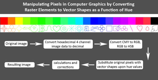
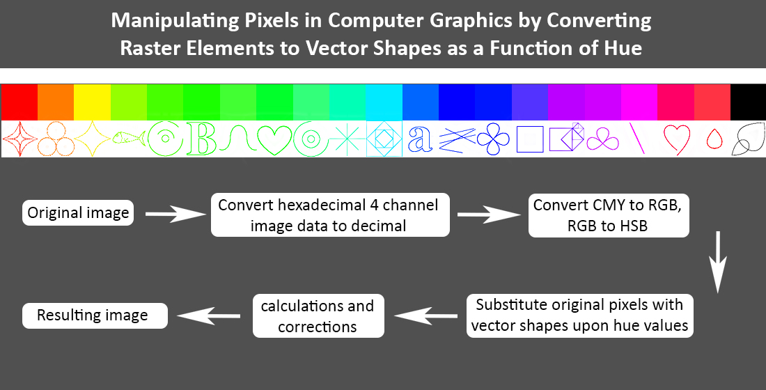
1. Introduction
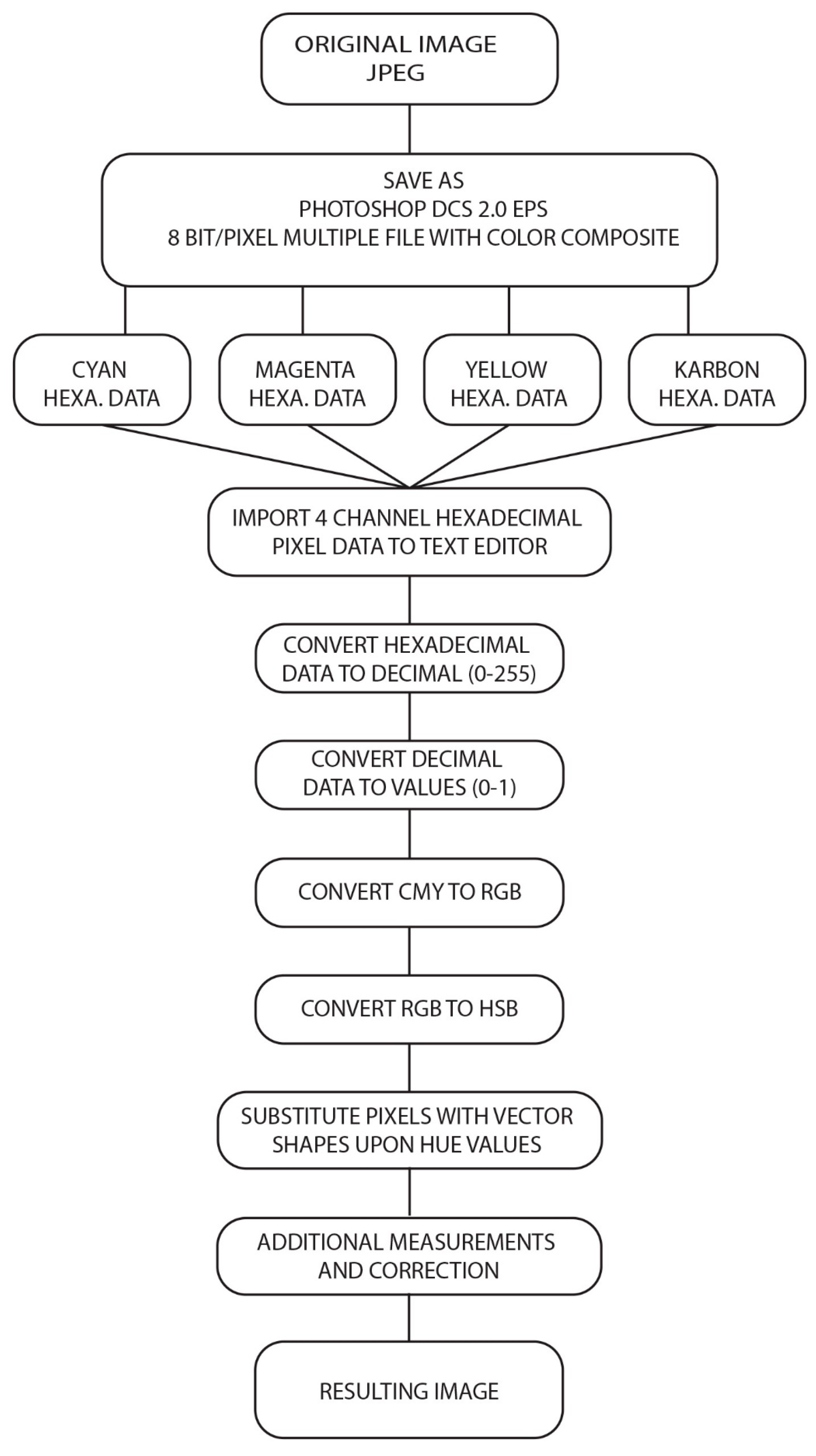
2. Materials and Methods
- -
- Define the width (w) and height (h) of the cell at the position of the original pixel;
- -
- Define the total number of columns (S) and rows (R) of the matrix;
- -
- Construct a matrix in which the cell positions x and y are defined as x = w × s; y = h × r, where ‘s’ and ‘r’ are the values of the current column and row.
M1 = M + K
Y1 = Y + K
K1 = K − K = 0
G = 1 − M1
B = 1 − Y1
For G = max, H = 2 + (B − R/Δmax–min) × 60/360
For B = max, H = 4 + (R − G/Δmax–min) × 60/360
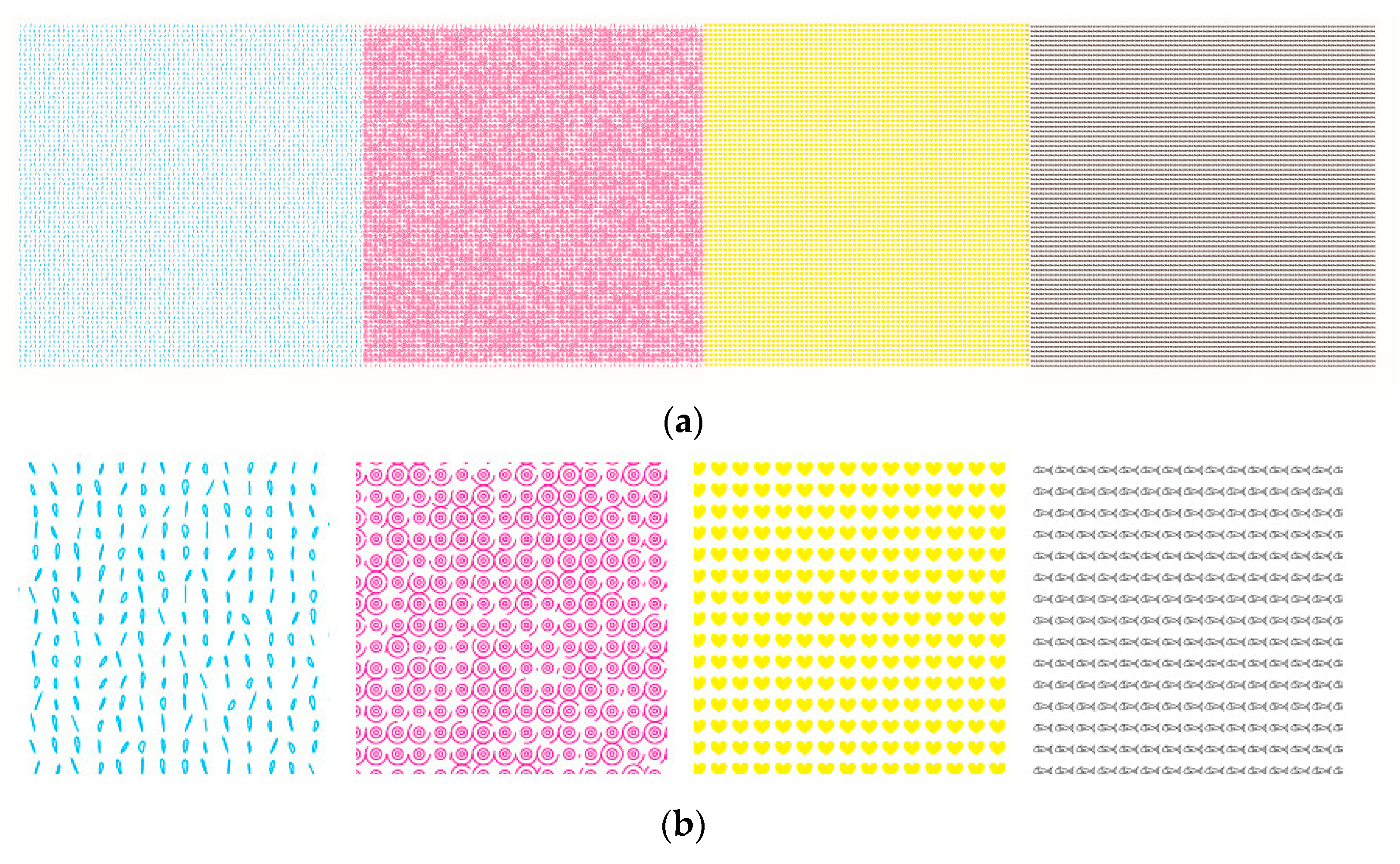
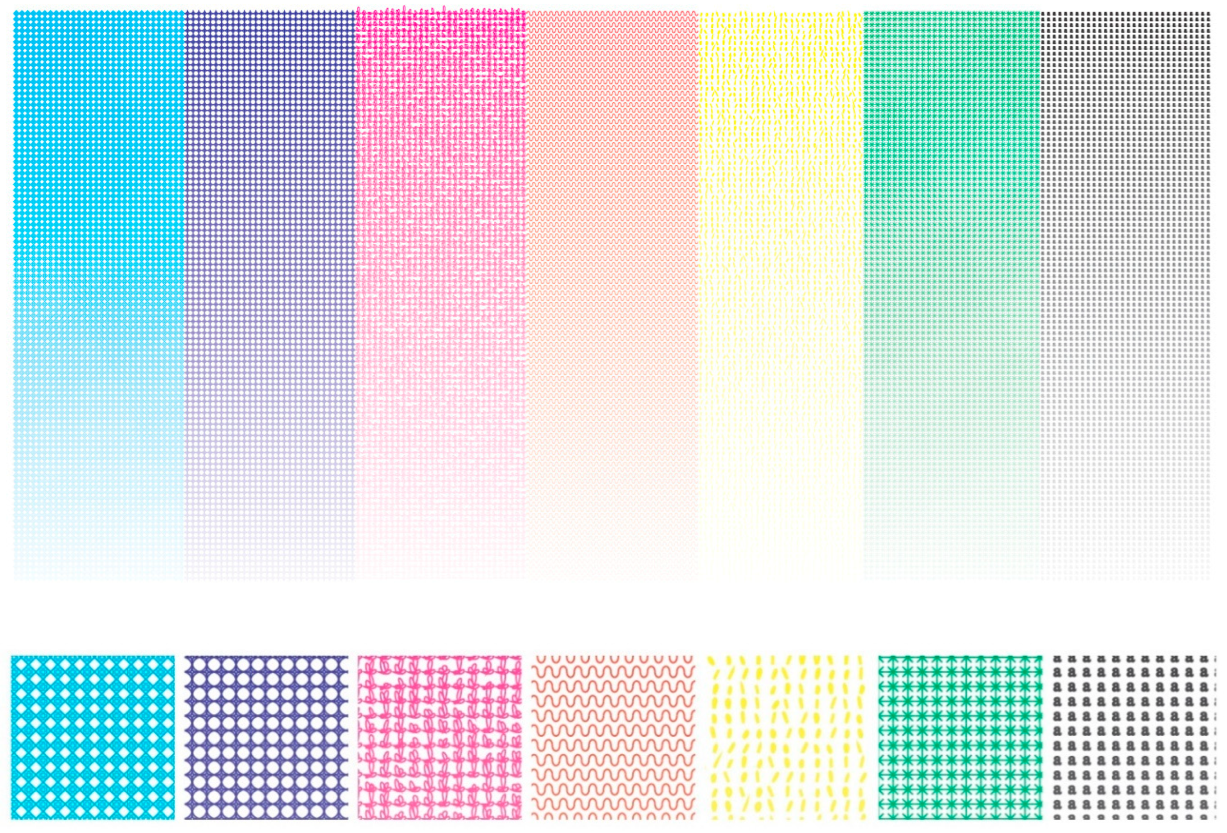
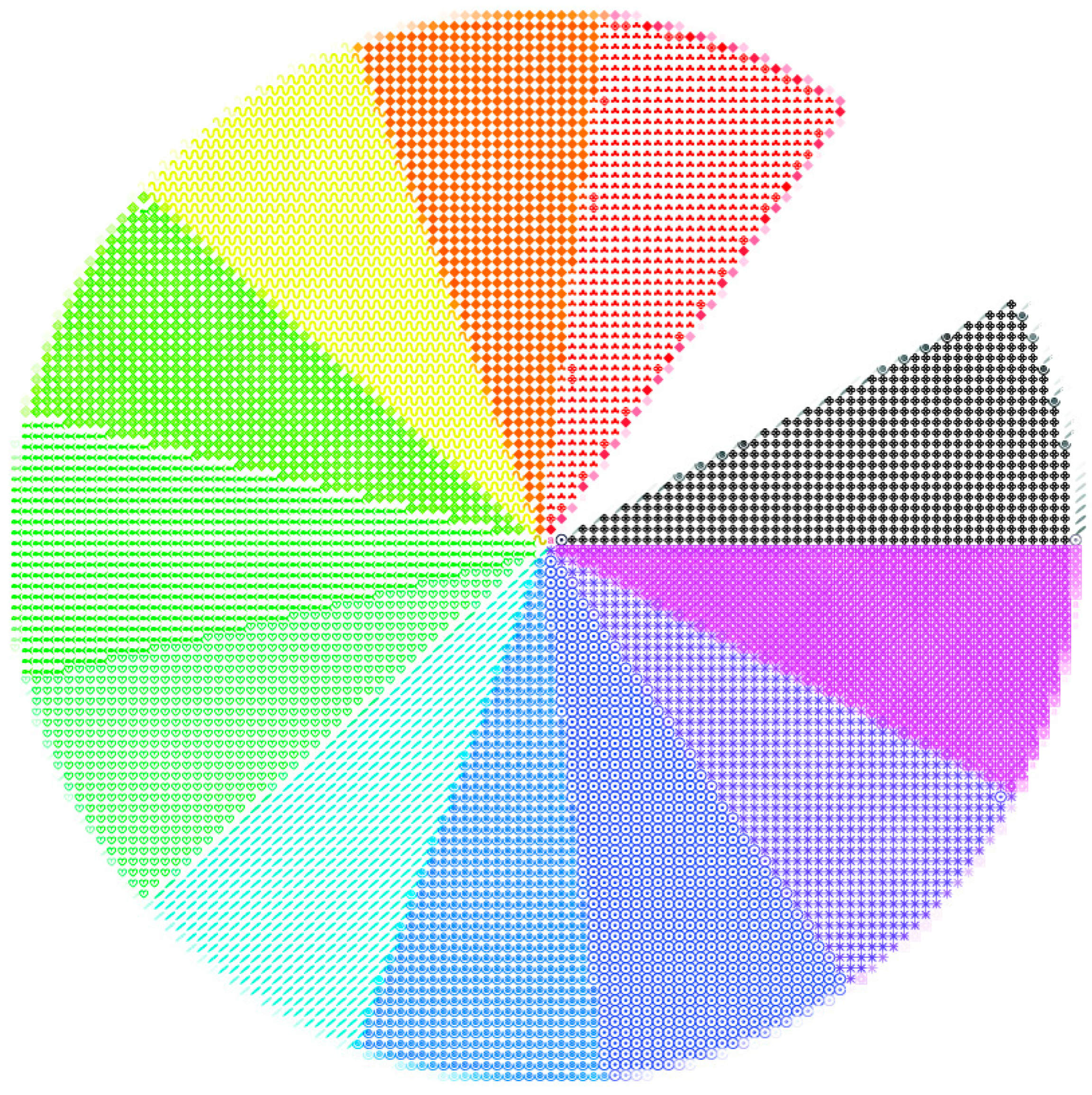
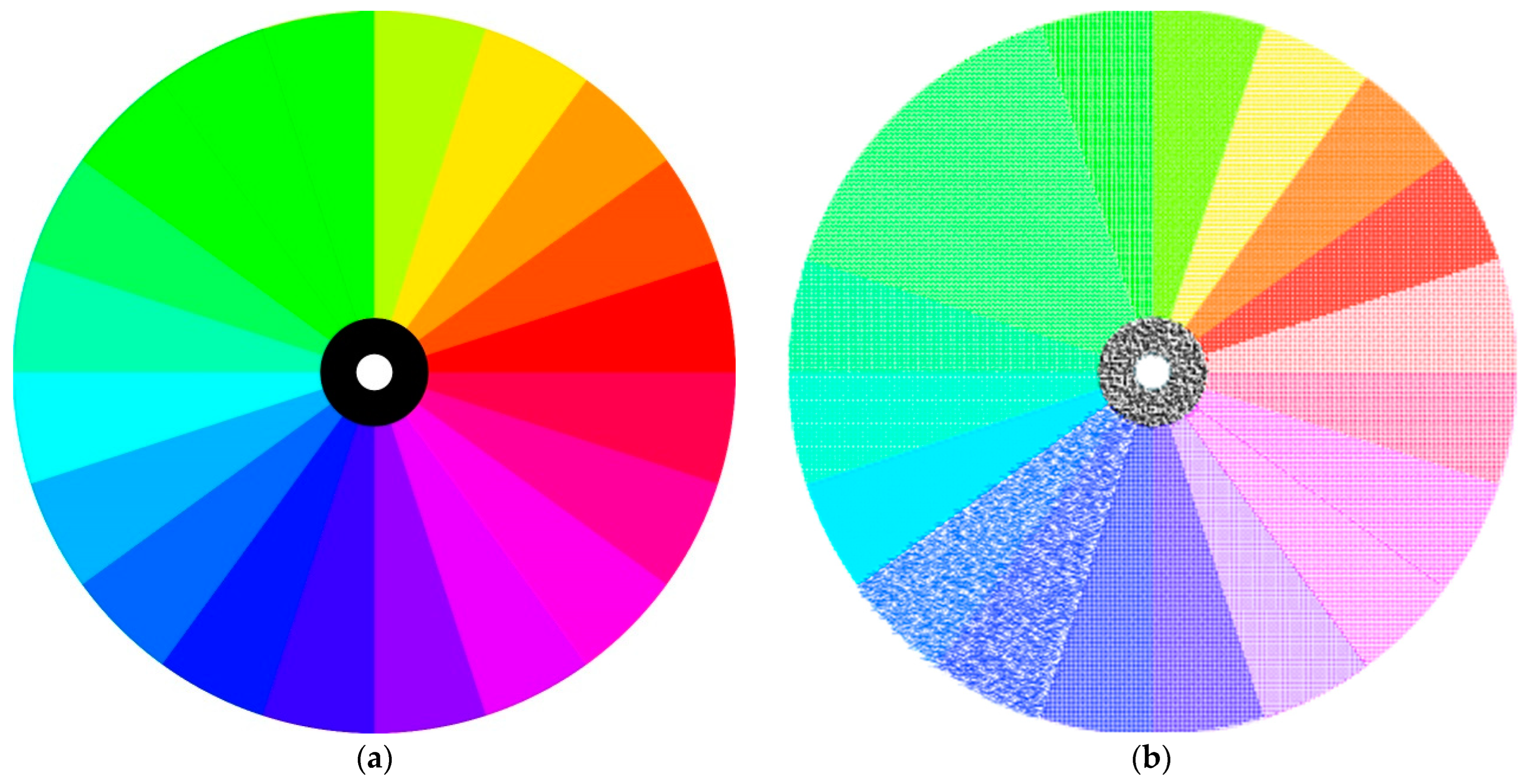
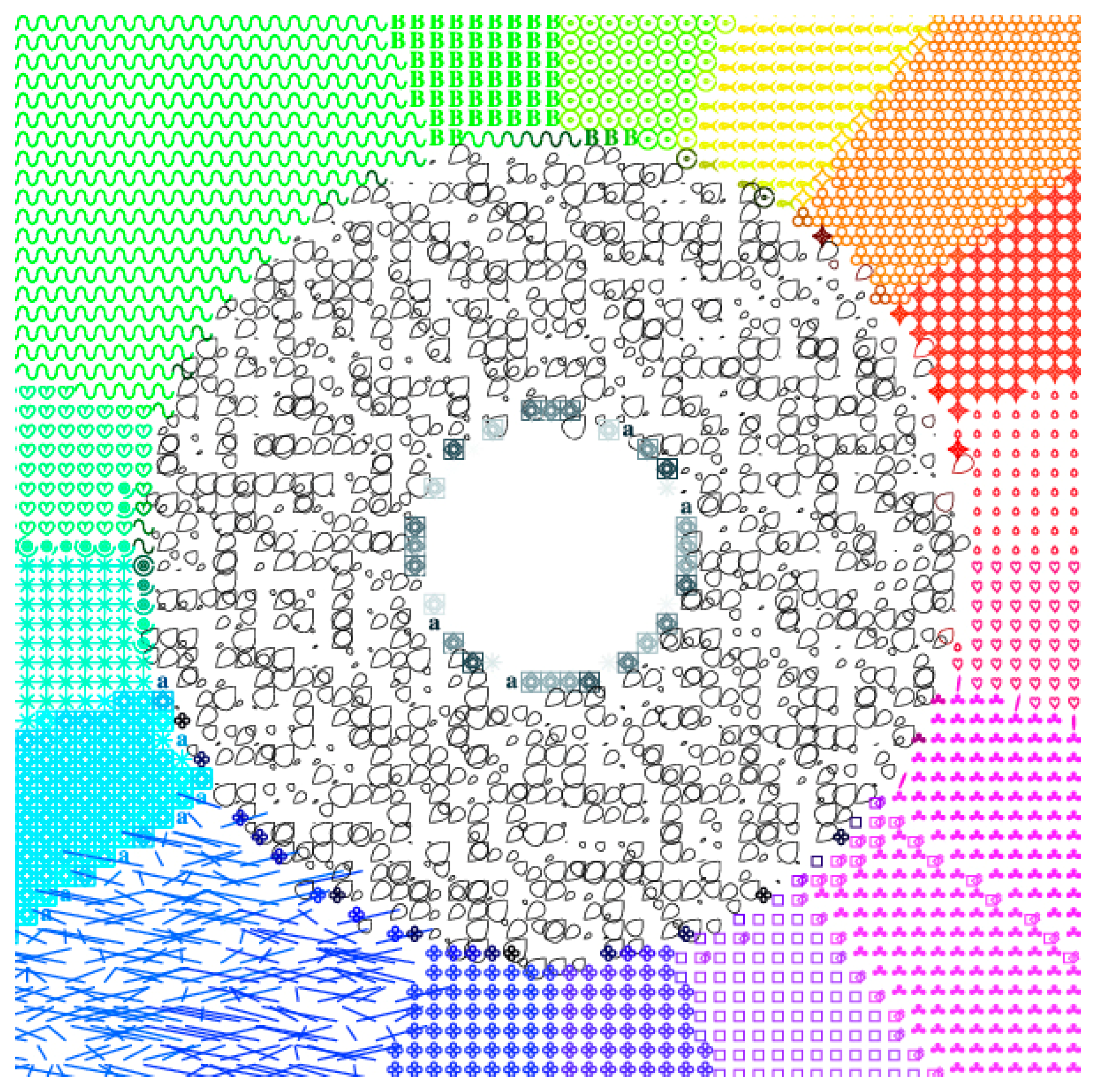
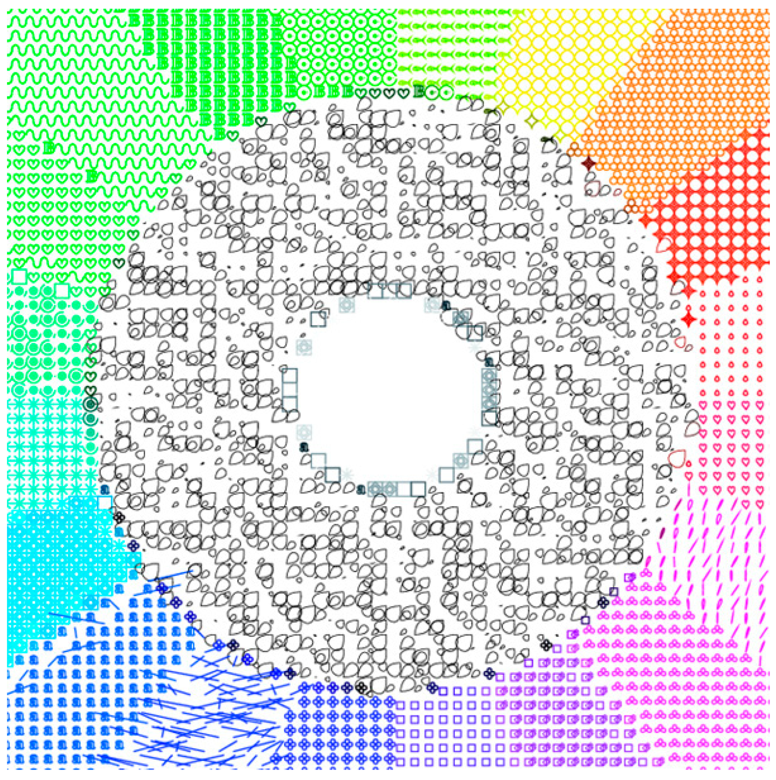
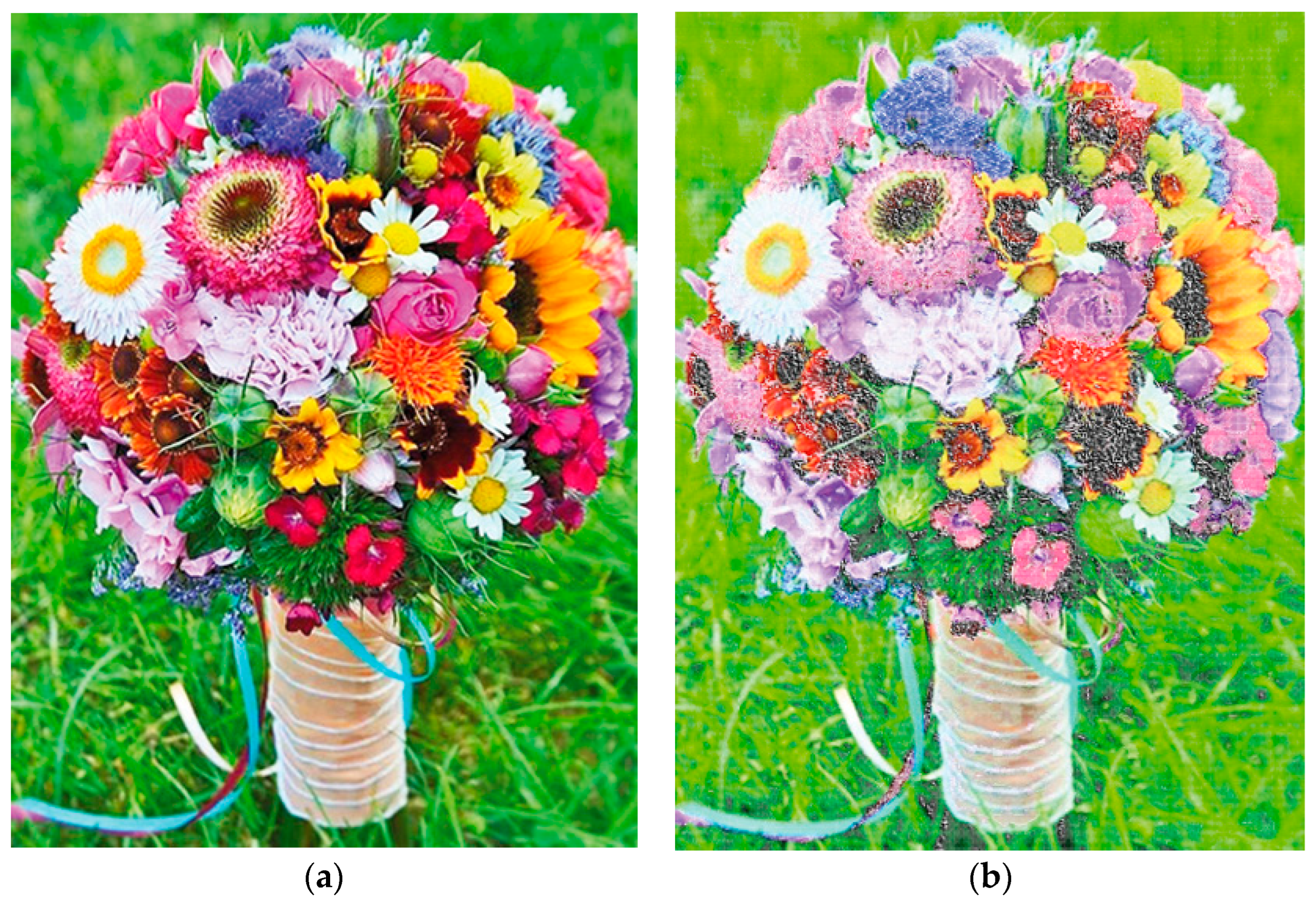
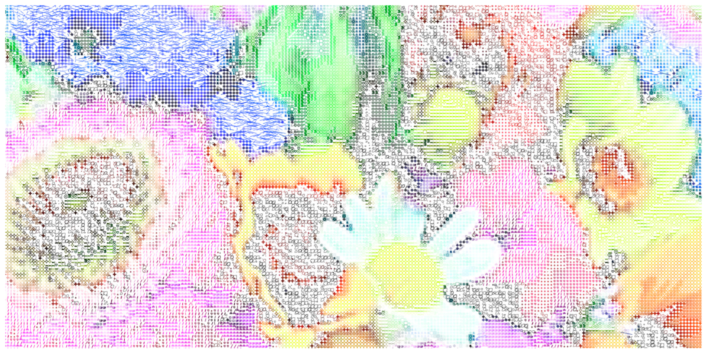
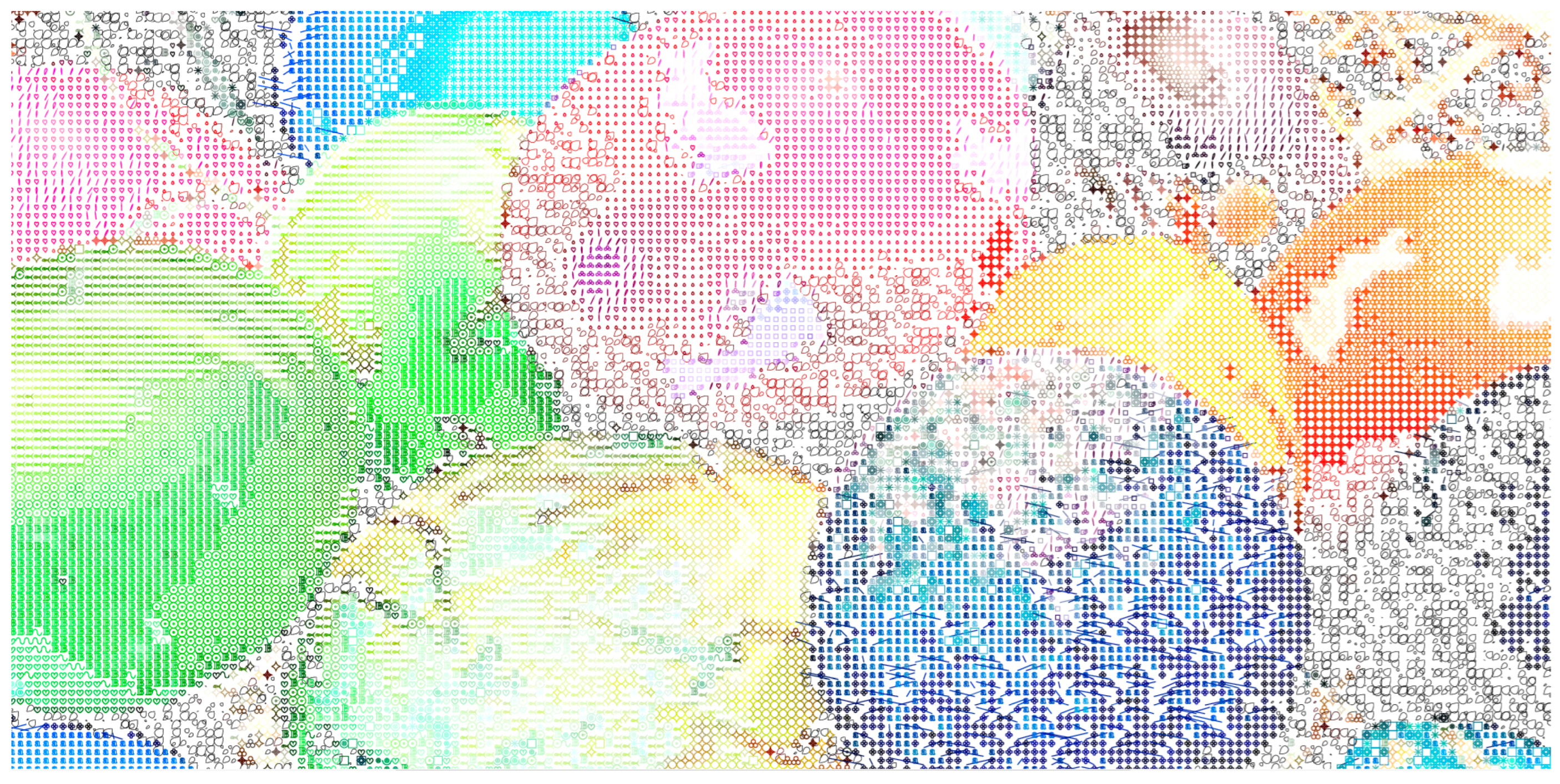
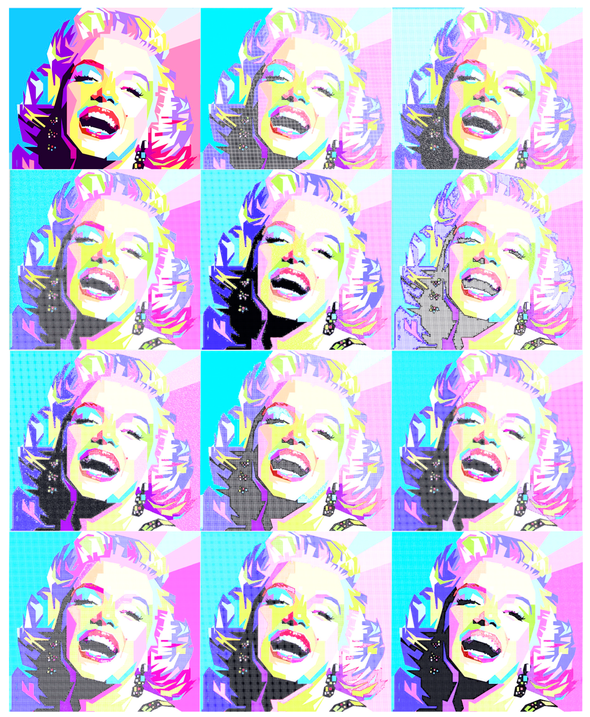
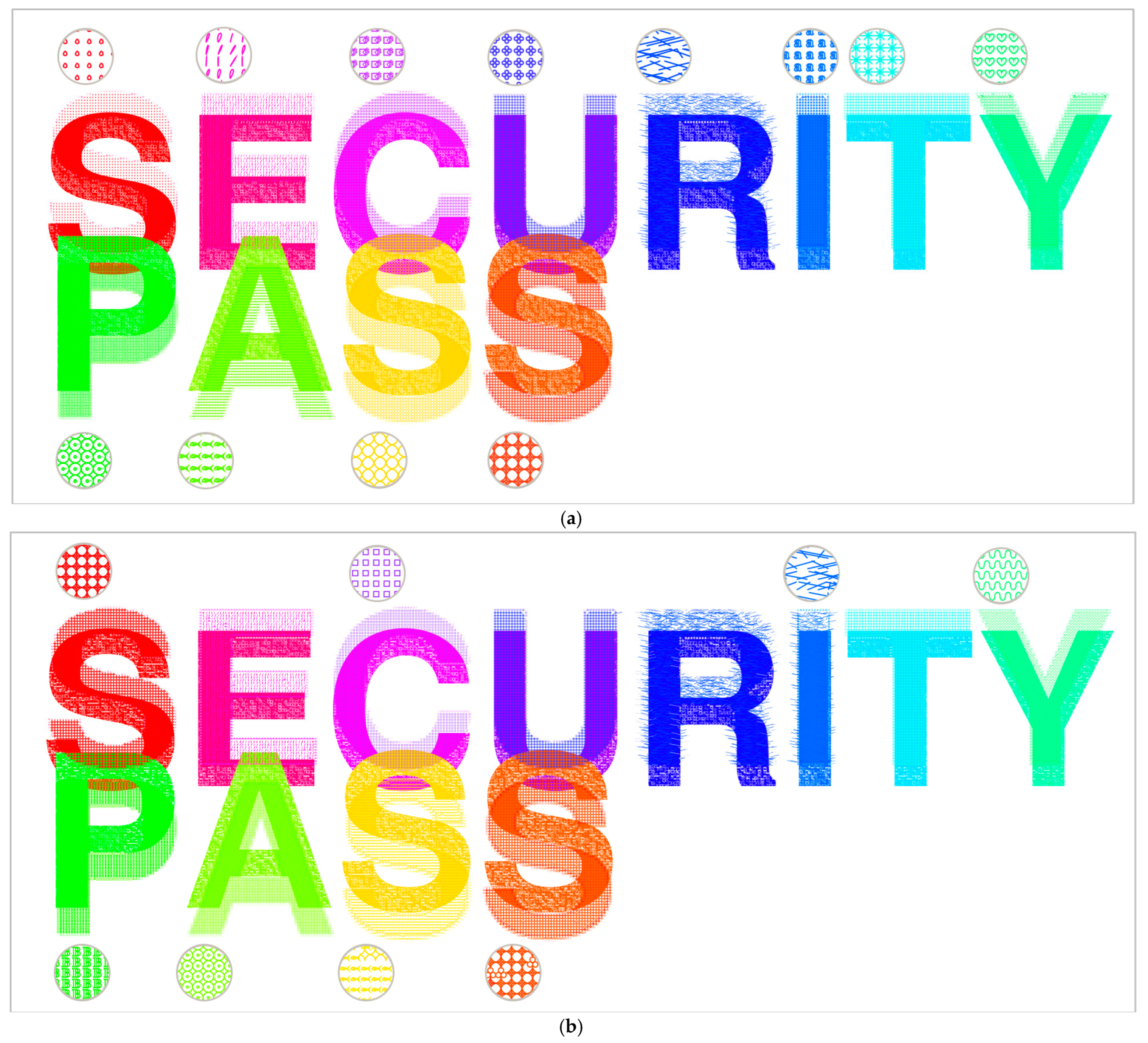
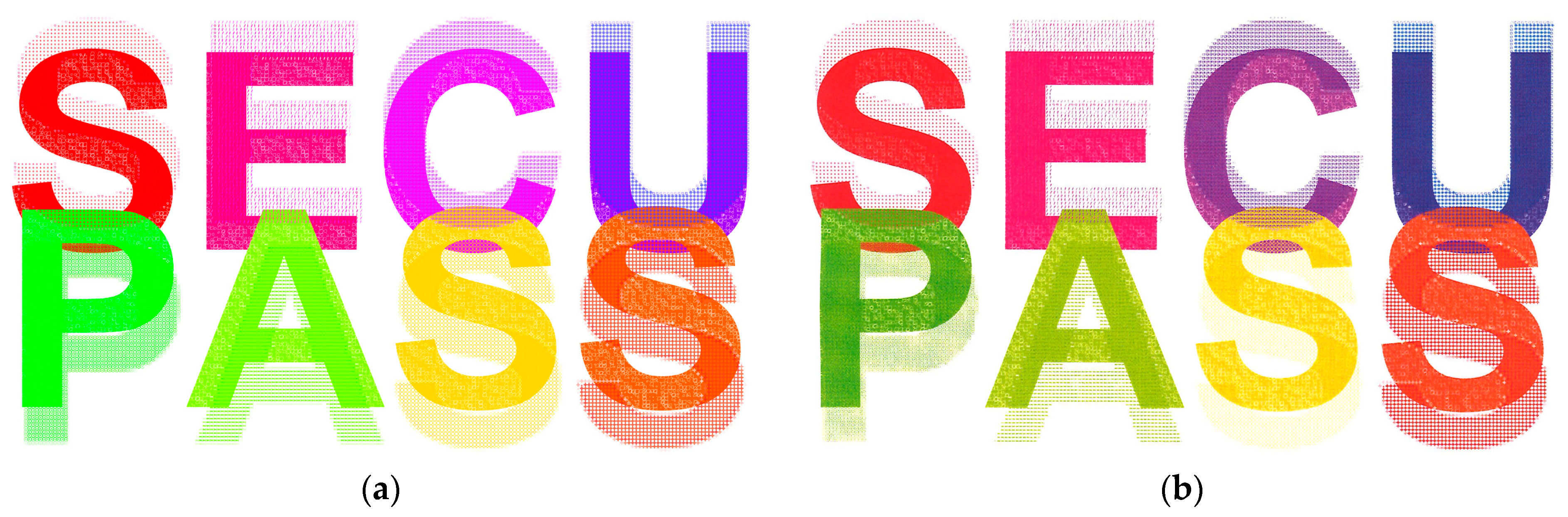
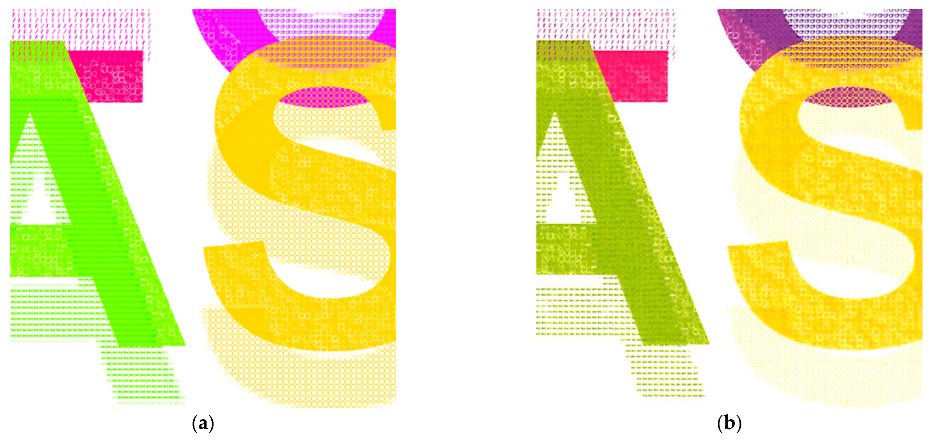
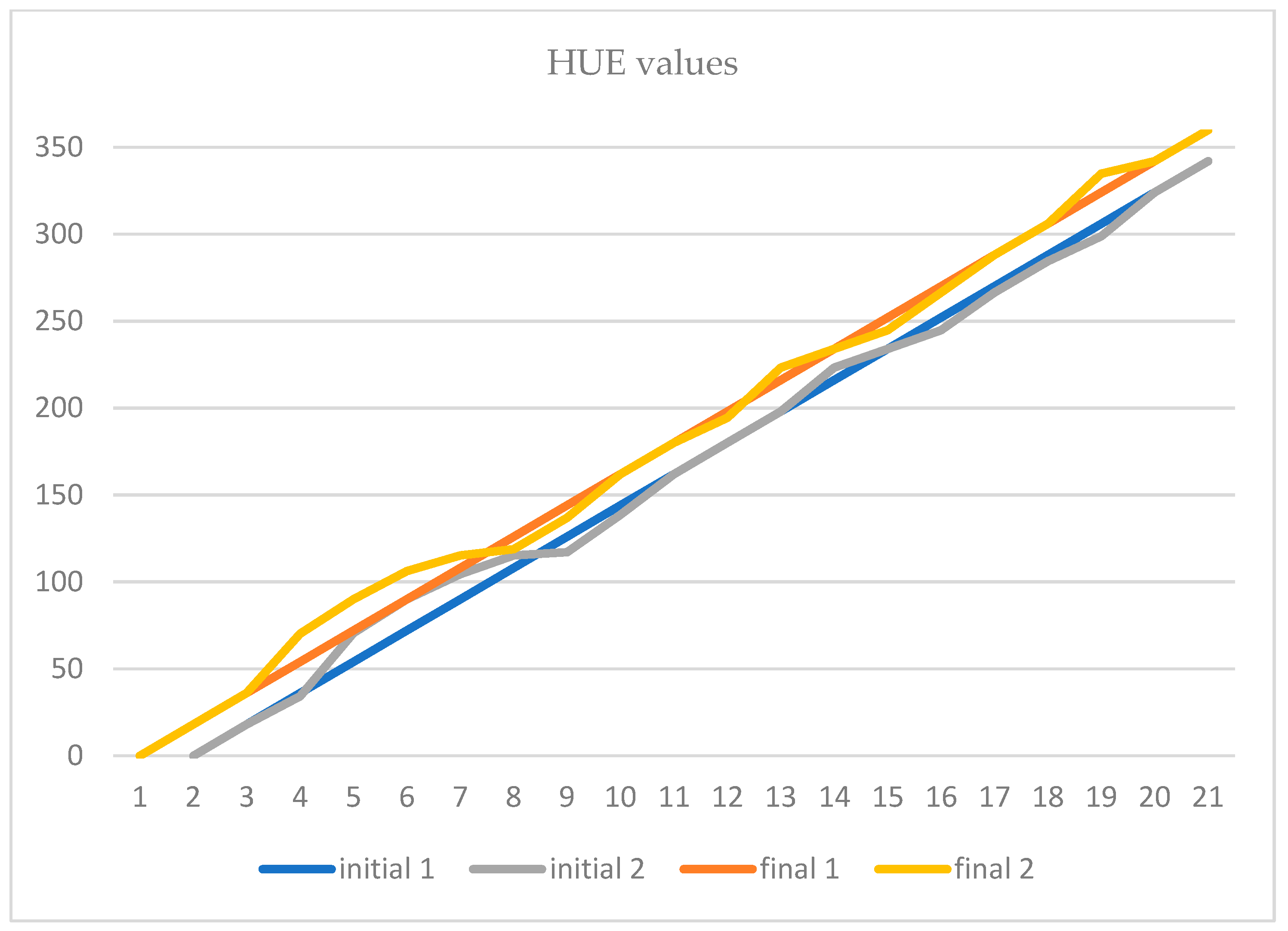
3. Results
4. Discussion and Conclusions
Supplementary Materials
Author Contributions
Funding
Institutional Review Board Statement
Informed Consent Statement
Data Availability Statement
Conflicts of Interest
References
- Ostromoukhov, V.; Hersch, R.D. Artistic Screening. In Proceedings of the SIGGRAPH’95: 22nd Annual Conference on Computer Graphics and Interactive Techniques, Los Angeles, CA, USA, 6–11 August 1995; pp. 219–228. [Google Scholar]
- Rudaz, N.; Hersch, R.D.; Ostromoukhov, V. An interface for the interactive design of artistic screens. In Electronic Publishing, Artistic Imaging and Digital Typography; Lecture Notes in Computer Science; Springer: Berlin/Heidelberg, Germany, 1998; Volume 1375, pp. 1–10. [Google Scholar]
- Ostromoukhov, V.; Rudaz, N.; Amidror, I.; Emmel, P.; Hersch, R.D. Anti-Counterfeiting Feature of Artistic Screening. In Holographic and Diffractive Techniques; SPIE: Bellingham, WA, USA, 1996; Volume 2951, pp. 126–133. [Google Scholar]
- Ostromoukhov, V. Mathematical Tools for Computer-Generated Ornamental Patterns. In Electronic Publishing, Artistic Imaging and Digital Typography; Lecture Notes in Computer Science; Springer: Berlin/Heidelberg, Germany, 1998; Volume 1375, pp. 193–223. [Google Scholar]
- Sugathan, S.; Scaria, R.; James, A.P. Adaptive Digital Scan Variable Pixels. In Proceedings of the 2015 International Conference on Advances in Computing, Communications and Informatics (ICACCI), Kochi, India, 10–13 August 2015. [Google Scholar]
- Sugathan, S.; James, A.P. Irregular pixel imaging. In Proceedings of the 2014 International Conference on Advances in Computing, Communications and Informatics (ICACCI), Delhi, India, 24–27 September 2014; pp. 2459–2463. [Google Scholar]
- Pap, K.; Žiljak, I.; Žiljak Vujić, J. Design of Digital Screening; FS Ltd.: Zagreb, Croatia, 2008. [Google Scholar]
- Koren, T.; Žiljak, V.; Rudolf, M.; Stanić Loknar, N.; Bernašek, A. Mathematical Models of the Sinusoidal Screen Family. Acta Graph. J. Print. Sci. Graph. Commun. 2017, 22, 11–20. [Google Scholar]
- Pap, K.; Žiljak Vujić, J.; Ziljak, I.; Agić, D. Screen Element Shape ‘R73’ Mutation. In DAAAM International Scientific Book; DAAAM International: Vienna, Austria, 2009; pp. 763–770. [Google Scholar]
- Ostromoukhov, V.; Hersch, R.D. Multi-Color and Artistic Dithering. In Proceedings of the SIGGRAPH 99: 26th Annual Conference on Computer Graphics and Interactive Techniques, Los Angeles, CA, USA, 8–13 August 1999; pp. 425–432. [Google Scholar]
- Kopf, J.; Lischinski, D. Depixelizing pixel art. ACM Trans. Graph. 2011, 30, 1–8. [Google Scholar] [CrossRef]
- Kabbai, L.; Sghaier, A.; Douik, A.; Machhout, M. FPGA implementation of filtered image using 2D Gaussian filter. Int. J. Adv. Comput. Sci. Appl. 2016, 7, 514–520. [Google Scholar] [CrossRef]
- Teutsch, M.; Trantelle, P.; Beyerer, J. Adaptive real-time image smoothing using local binary patterns and Gaussian filters. In Proceedings of the 2013 IEEE International Conference on Image Processing, Melbourne, VIC, Australia, 15–18 September 2013; pp. 1120–1124. [Google Scholar]
- Yang, C.; Liu, C.; Shen, C. Guided Gaussian range kernel filtering based on similarity-aware window. J. Electron. Imaging 2022, 31, 043022. [Google Scholar] [CrossRef]
- Wei, Z.; Yan, Q.; Lu, X.; Zheng, Y.; Sun, S.; Lin, J. Compression Reconstruction Network with Coordinated Self-Attention and Adaptive Gaussian Filtering Module. Mathematics 2023, 11, 847. [Google Scholar] [CrossRef]
- Aurich, V.; Weule, J. Non-Linear Gaussian Filters Performing Edge Preserving Diffusion. In Mustererkennung 1995; Sagerer, G., Posch, S., Kummert, F., Eds.; Informatik Aktuell; Springer: Berlin/Heidelberg, Germany, 1995. [Google Scholar]
- Smith, S.M.; Brady, J.M. SUSAN—A New Approach to Low Level Image Processing. Int. J. Comput. Vis. 1997, 23, 45–78. [Google Scholar] [CrossRef]
- Tomasi, C.; Manduchi, R. Bilateral filtering for gray and color images. In Proceedings of the Sixth International Conference on Computer Vision (IEEE Cat. No.98CH36271), Bombay, India, 7 January 1998; pp. 839–846. [Google Scholar]
- Cheng, S.W.; Lin, Y.T.; Peng, Y.T. A Fast Two-Stage Bilateral Filter Using Constant Time O(1) Histogram Generation. Sensors 2022, 22, 926. [Google Scholar] [CrossRef] [PubMed]
- Petschnigg, G.; Agrawala, M.; Hoppe, H.; Szeliski, R.; Cohen, M.; Toyama, K. Digital Photography with Flash and No-Flash Image Pairs; Association for Computing Machinery: New York, NY, USA, 2004; Volume 23, pp. 664–672. [Google Scholar]
- Eisemann, E.; Durand, F. Flash Photography Enhancement via Intrinsic Relighting; Association for Computing Machinery: New York, NY, USA, 2004; Volume 23, pp. 673–678. [Google Scholar]
- Choudhury, P.; Tumblin, J. The Trilateral Filter for High Contrast Images and Meshes; Association for Computing Machinery: New York, NY, USA, 2005; p. 5–es. [Google Scholar]
- Ji, G.; Wang, Z.; Zhou, L.; Xia, Y.; Zhong, S.; Gong, S. SAR Image Colorization Using Multidomain Cycle-Consistency Generative Adversarial Network. IEEE Geosci. Remote Sens. Lett. 2021, 18, 296–300. [Google Scholar] [CrossRef]
- Koukiou, G. Perceptually Optimal Color Representation of Fully Polarimetric SAR Imagery. J. Imaging 2022, 8, 67. [Google Scholar] [CrossRef] [PubMed]
- Inoue, K.; Jiang, M.; Hara, K. Hue-Preserving Saturation Improvement in RGB Color Cube. J. Imaging 2021, 7, 150. [Google Scholar] [CrossRef] [PubMed]
- Guo, G.; Han, T.; Wu, B.; Fu, J.; Xia, Z. A hue preservation lossless contrast enhancement method with RDH for color images. Digit. Signal Process. 2023, 136, 103965. [Google Scholar] [CrossRef]
- Moussa, M.I.; Abd El-Latif, E.I.; Majid, N. Enhancing the Security of Digital Image Encryption using Diagonalize Multidimensional Nonlinear Chaotic System. Int. J. Adv. Comput. Sci. Appl. (IJACSA) 2022, 13, 524–533. [Google Scholar] [CrossRef]
- Razzaq, M.A.; Shaikh, R.A.; Baig, M.A.; Memon, A.A. Digital Image Security: Fusion of Encryption, Steganography and Watermarking. Int. J. Adv. Comput. Sci. Appl. (IJACSA) 2017, 8, 224–228. [Google Scholar]
- Zhang, S.; Liu, L. A novel image encryption algorithm based on SPWLCM and DNA coding. Math. Comput. Simul. 2021, 190, 723–744. [Google Scholar] [CrossRef]
- Dronyuk, I.; Kalinchuk, V.; Greguš, M. Protection of images based on fractal geometry. Procedia Comput. Sci. 2019, 160, 515–520. [Google Scholar] [CrossRef]
- Hussein, Q.M.; Abdullah, A.S.; Mohammed, N.Q. The efficiency of Color Models layers at Color Images as Cover in text hiding. Tikrit J. Pure Sci. 2016, 21, 130–139. [Google Scholar] [CrossRef]
- Shevell, S.K. The Science of Color, 2nd ed.; Elsevier: Oxford, UK, 2003; pp. 192–197. [Google Scholar]
- Saravanan, G.; Yamuna, G.; Nandhini, S. Real time implementation of RGB to HSV/HSI/HSL and its reverse color space models. In Proceedings of the 2016 International Conference on Communication and Signal Processing (ICCSP), Melmaruvathur, India, 6–8 April 2016; pp. 462–466. [Google Scholar]
- Huang, Z.K.; Liu, D.H. Segmentation of Color Image Using EM algorithm in HSV Color Space. In Proceedings of the 2007 International Conference on Information Acquisition, Seogwipo, Republic of Korea, 8–11 July 2007; pp. 316–319. [Google Scholar]
- Converting RGB to HSV. Available online: https://mattlockyer.github.io/iat455/documents/rgb-hsv.pdf (accessed on 1 October 2022).
- Ford, A.; Roberts, A. Colour Space Conversions. 1998, pp. 11–17. Available online: https://poynton.ca/PDFs/coloureq.pdf (accessed on 22 December 2022).
- Gomes, J.; Velho, L.; Costa Sousa, M. Computer Graphics: Theory and Practice, 1st ed.; Peters, A.K., Ed.; CRC Press: New York, NY, USA, 2012; pp. 108–136. [Google Scholar] [CrossRef]
- Žiljak, V.; Pap, K. Postscript Programiranje; FS Ltd.: Zagreb, Croatia, 1999. [Google Scholar]
- Reid, G.C. Thinking in PostScrıpt®; Addison-Wesley Publishing Company: Boston, MA, USA, 1990. [Google Scholar]
- Michael, L. Scott Programming Language Pragmatics, 2nd ed.; Morgan Kaufmann Publishers: San Francisco, CA, USA, 2006; pp. 679–767. [Google Scholar]
- Adobe Systems Incorporated PostScript® LANGUAGE REFERENCE, 3rd ed.; Addison-Wesley Publishing Company: Boston, MA, USA, 1999; Retrieved 18 June 2004; Available online: https://www.adobe.com/jp/print/postscript/pdfs/PLRM.pdf (accessed on 2 December 2022).


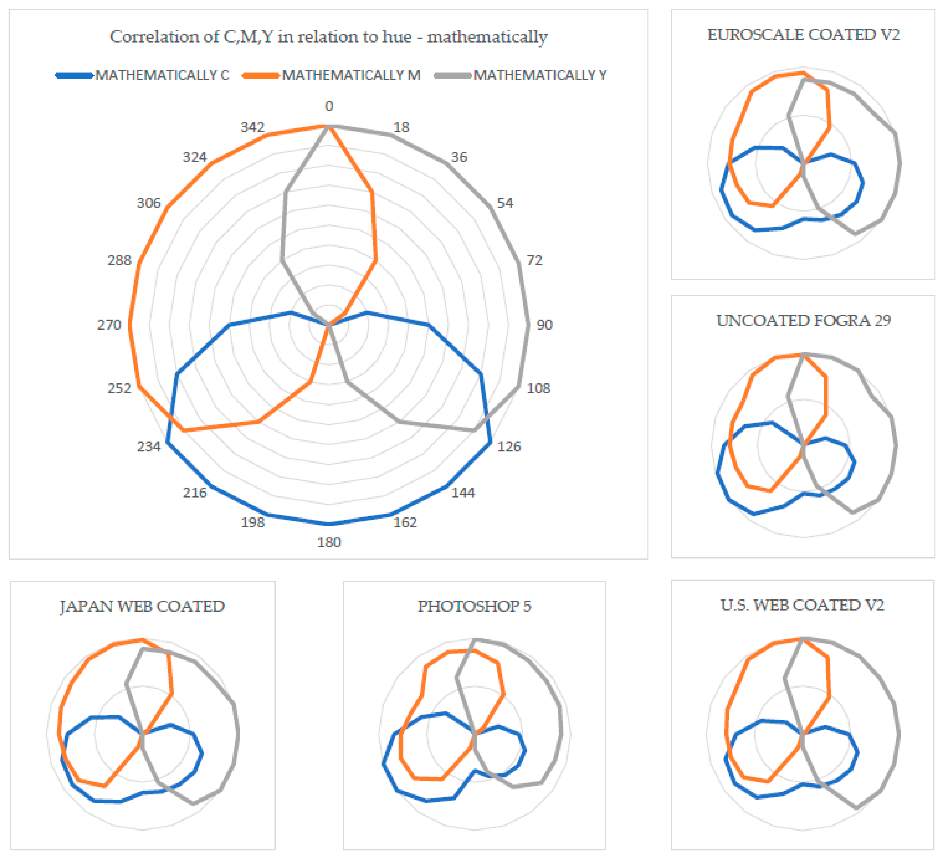
| Mathematecally | Euroscale Coated V2 | Uncoated Fogra 29 | |||||||||
|---|---|---|---|---|---|---|---|---|---|---|---|
| H | C | M | Y | H | C | M | Y | H | C | M | Y |
| 0 | 0 | 100 | 100 | 0 | 0 | 94 | 87 | 0 | 0 | 98 | 99 |
| 18 | 0 | 70 | 100 | 18 | 0 | 80 | 88 | 18 | 0 | 78 | 100 |
| 36 | 0 | 40 | 100 | 36 | 0 | 46 | 89 | 36 | 0 | 41 | 100 |
| 54 | 0 | 10 | 100 | 54 | 2 | 4 | 89 | 54 | 3 | 1 | 91 |
| 72 | 20 | 0 | 100 | 72 | 30 | 0 | 100 | 72 | 25 | 0 | 100 |
| 90 | 50 | 0 | 100 | 90 | 53 | 0 | 100 | 90 | 45 | 0 | 100 |
| 108 | 80 | 0 | 100 | 108 | 65 | 0 | 100 | 108 | 58 | 0 | 100 |
| 126 | 100 | 0 | 90 | 126 | 68 | 0 | 100 | 126 | 60 | 0 | 100 |
| 144 | 100 | 0 | 60 | 144 | 66 | 0 | 91 | 144 | 58 | 0 | 90 |
| 162 | 100 | 0 | 30 | 162 | 62 | 0 | 49 | 162 | 57 | 0 | 46 |
| 180 | 100 | 0 | 0 | 180 | 58 | 0 | 14 | 180 | 52 | 0 | 12 |
| 198 | 100 | 30 | 0 | 198 | 71 | 12 | 0 | 198 | 69 | 13 | 0 |
| 216 | 100 | 60 | 0 | 216 | 86 | 55 | 0 | 216 | 92 | 61 | 0 |
| 234 | 100 | 90 | 0 | 234 | 92 | 70 | 0 | 234 | 100 | 75 | 0 |
| 252 | 80 | 100 | 0 | 252 | 90 | 73 | 0 | 252 | 98 | 77 | 0 |
| 270 | 50 | 100 | 0 | 270 | 78 | 77 | 0 | 270 | 86 | 80 | 0 |
| 288 | 20 | 100 | 0 | 288 | 53 | 78 | 0 | 288 | 67 | 81 | 0 |
| 306 | 0 | 100 | 10 | 306 | 27 | 80 | 0 | 306 | 42 | 81 | 0 |
| 324 | 0 | 100 | 40 | 324 | 0 | 92 | 0 | 324 | 3 | 94 | 0 |
| 342 | 0 | 100 | 70 | 342 | 0 | 95 | 52 | 342 | 0 | 100 | 56 |
| Japan Web Coated | Photoshop 5 | Web Coated V2 U.S. | |||||||||
| H | C | M | Y | H | C | M | Y | H | C | M | Y |
| 0 | 0 | 98 | 89 | 0 | 0 | 87 | 99 | 0 | 0 | 99 | 100 |
| 18 | 0 | 88 | 90 | 18 | 0 | 78 | 98 | 18 | 0 | 84 | 100 |
| 36 | 0 | 52 | 93 | 36 | 0 | 51 | 95 | 36 | 0 | 47 | 100 |
| 54 | 2 | 7 | 93 | 54 | 1 | 11 | 93 | 54 | 2 | 4 | 99 |
| 72 | 31 | 0 | 100 | 72 | 26 | 0 | 93 | 72 | 25 | 0 | 100 |
| 90 | 53 | 0 | 100 | 90 | 46 | 0 | 90 | 90 | 48 | 0 | 100 |
| 108 | 65 | 0 | 100 | 108 | 55 | 0 | 88 | 108 | 60 | 0 | 100 |
| 126 | 67 | 0 | 100 | 126 | 56 | 0 | 86 | 126 | 62 | 0 | 100 |
| 144 | 65 | 0 | 90 | 144 | 53 | 0 | 68 | 144 | 60 | 0 | 95 |
| 162 | 63 | 0 | 53 | 162 | 46 | 0 | 41 | 162 | 57 | 0 | 51 |
| 180 | 61 | 0 | 15 | 180 | 38 | 0 | 16 | 180 | 52 | 0 | 13 |
| 198 | 74 | 14 | 0 | 198 | 70 | 15 | 0 | 198 | 65 | 15 | 0 |
| 216 | 86 | 67 | 0 | 216 | 86 | 58 | 0 | 216 | 81 | 61 | 0 |
| 234 | 90 | 82 | 0 | 234 | 100 | 78 | 0 | 234 | 87 | 76 | 0 |
| 252 | 88 | 84 | 0 | 252 | 100 | 81 | 0 | 252 | 84 | 78 | 0 |
| 270 | 78 | 87 | 0 | 270 | 84 | 77 | 0 | 270 | 69 | 79 | 0 |
| 288 | 56 | 89 | 0 | 288 | 58 | 70 | 0 | 288 | 45 | 82 | 0 |
| 306 | 30 | 91 | 0 | 306 | 37 | 68 | 0 | 306 | 21 | 84 | 0 |
| 324 | 0 | 96 | 0 | 324 | 6 | 87 | 0 | 324 | 0 | 96 | 0 |
| 342 | 0 | 98 | 55 | 342 | 0 | 90 | 62 | 342 | 0 | 99 | 61 |
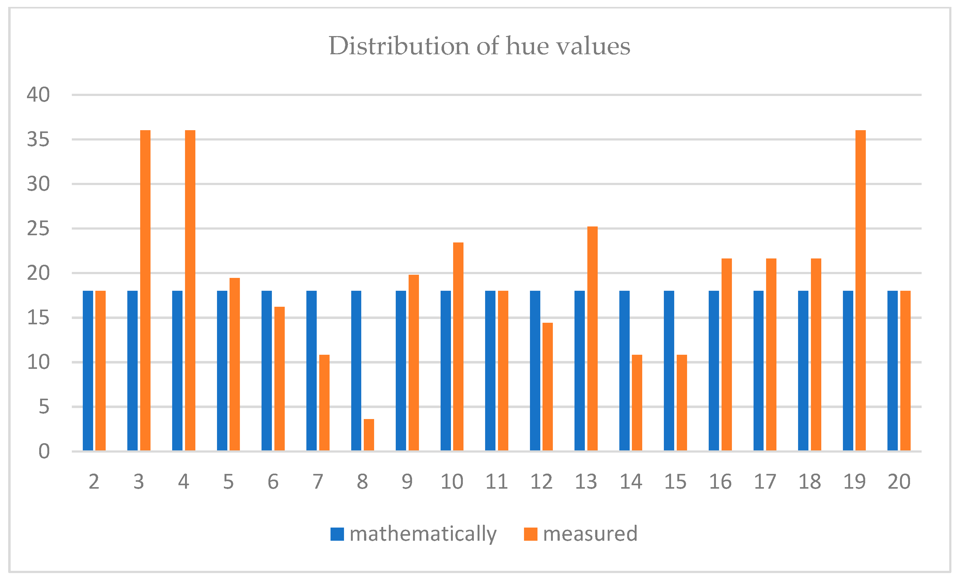
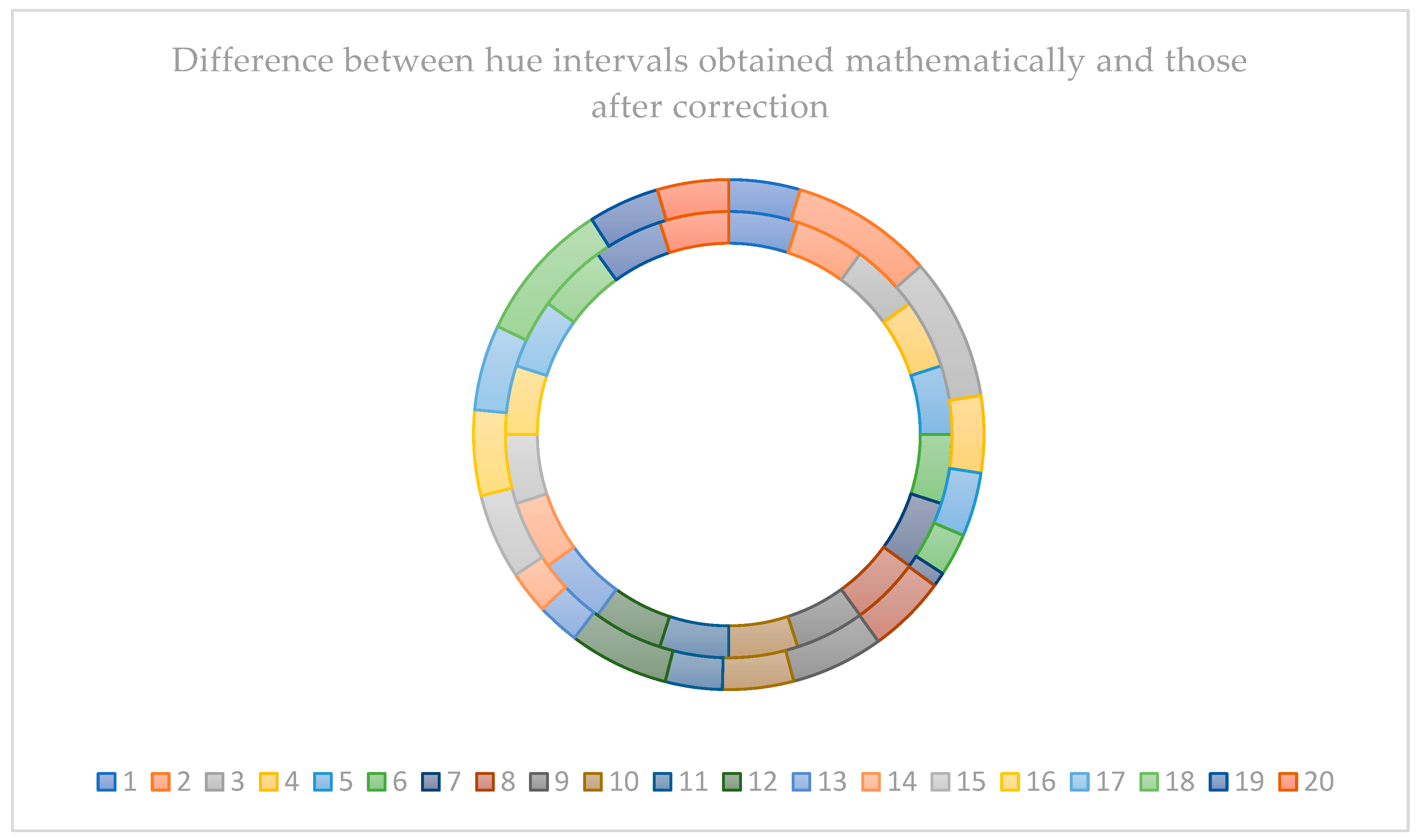
| H Mathematically (Degrees) | H Mathematically (Values 0–1) | Interval (Degrees) | H Displaying Correctly (Degrees) | H Displaying Correctly (Values 0–1) | Interval (Degrees) | |
|---|---|---|---|---|---|---|
| 1 | 0–18 | 0–0.05 | 18 | 0–18 | 0–0.05 | 18 |
| 2 | 18–36 | 0.05–0.1 | 18 | 18–36 | 0.05–0.01 | 36 |
| 3 | 36–54 | 0.1–0.15 | 18 | 34.2–70.2 | 0.095–0.195 | 36 |
| 4 | 54–72 | 0.15–0.2 | 18 | 70.56–90 | 0.196–0.25 | 19.44 |
| 5 | 72–90 | 0.2–0.25 | 18 | 90–106.2 | 0.25–0.295 | 16.2 |
| 6 | 90–108 | 0.25–0.3 | 18 | 104.4–115.2 | 0.29–0.32 | 10.8 |
| 7 | 108–126 | 0.3–0.35 | 18 | 115.2–118.8 | 0.32–0.33 | 3.6 |
| 8 | 126–144 | 0.35–0.4 | 18 | 117–136.8 | 0.325–0.38 | 19.8 |
| 9 | 144–162 | 0.4–0.45 | 18 | 138.6–162 | 0.385–0.45 | 23.4 |
| 10 | 162–180 | 0.45–0.5 | 18 | 162–180 | 0.45–0.5 | 18 |
| 11 | 180–198 | 0.5–0.55 | 18 | 180–194.4 | 0.5–0.54 | 14.4 |
| 12 | 198–216 | 0.55–0.6 | 18 | 198–223.2 | 0.55–0.62 | 25.2 |
| 13 | 216–234 | 0.6–0.65 | 18 | 223.2–234 | 0.62–0.65 | 10.8 |
| 14 | 234–252 | 0.65–0.7 | 18 | 234–244.8 | 0.65–0.68 | 10.8 |
| 15 | 252–270 | 0.7–0.75 | 18 | 244.8–266.4 | 0.68–0.74 | 21.6 |
| 16 | 270–288 | 0.75–0.8 | 18 | 266.4–288 | 0.74–0.8 | 21.6 |
| 17 | 288–306 | 0.8–0.85 | 18 | 284.4–306 | 0.79–0.85 | 21.6 |
| 18 | 306–324 | 0.85–0.9 | 18 | 298.8–334.8 | 0.83–0.93 | 36 |
| 19 | 324–342 | 0.9–0.95 | 18 | 324–342 | 0.9–0.95 | 18 |
| 20 | 342–360 | 0.95–1 | 18 | 342–360 | 0.95–1 | 18 |
Disclaimer/Publisher’s Note: The statements, opinions and data contained in all publications are solely those of the individual author(s) and contributor(s) and not of MDPI and/or the editor(s). MDPI and/or the editor(s) disclaim responsibility for any injury to people or property resulting from any ideas, methods, instructions or products referred to in the content. |
© 2023 by the authors. Licensee MDPI, Basel, Switzerland. This article is an open access article distributed under the terms and conditions of the Creative Commons Attribution (CC BY) license (https://creativecommons.org/licenses/by/4.0/).
Share and Cite
Koren Ivančević, T.; Stanić Loknar, N.; Rudolf, M.; Bratić, D. Manipulating Pixels in Computer Graphics by Converting Raster Elements to Vector Shapes as a Function of Hue. J. Imaging 2023, 9, 106. https://doi.org/10.3390/jimaging9060106
Koren Ivančević T, Stanić Loknar N, Rudolf M, Bratić D. Manipulating Pixels in Computer Graphics by Converting Raster Elements to Vector Shapes as a Function of Hue. Journal of Imaging. 2023; 9(6):106. https://doi.org/10.3390/jimaging9060106
Chicago/Turabian StyleKoren Ivančević, Tajana, Nikolina Stanić Loknar, Maja Rudolf, and Diana Bratić. 2023. "Manipulating Pixels in Computer Graphics by Converting Raster Elements to Vector Shapes as a Function of Hue" Journal of Imaging 9, no. 6: 106. https://doi.org/10.3390/jimaging9060106