
Multispectral Satellite Image Analysis for Computing Vegetation Indices by R in the Khartoum Region of Sudan, Northeast Africa


Abstract
:1. Introduction
1.1. Background
1.2. Objectives and Motivation
- To the best of our knowledge, this is the first paper in the literature that focuses on the application of R libraries for computing several vegetation indices over the area of Khartoum, Sudan;
- As opposed to previous studies, we present the application of ‘raster’ and ‘terra’ packages of R for remote sensing data analysis instead of the traditional GIS software;
- We further extend the use of Landsat 8–9 OLI/TIRS sensors to extract geospatial information from multispectral images;
- We comprehensively evaluate the performance of different vegetation indices for the case of semi-arid vegetation patterns in southern Sudan. To this end, we apply the R algorithms to calculate five different VI which differ in computational approaches and tuned to diverse environmental aspects of vegetation: (1) Normalised Difference Vegetation Index (NDVI); (2) Normalised Difference Water Index (NDWI); (3) Infrared Percentage Vegetation Index (IPVI); (4) Optimised Soil-Adjusted Vegetation Index (OSAVI); and (5) Green Normalised Difference Vegetation Index (GNDVI);
- We provide an overview of the major environmental aspects of Sudan which include recent issues of desertification related to semi-arid climate, land cover changes and hydrology of the Nile which controls the cycle of vegetation growth in Sudan.
- A summary of R scripts used for computing and mapping vegetation indices is reported, to provide the reader with the technical reference of the applied methods.
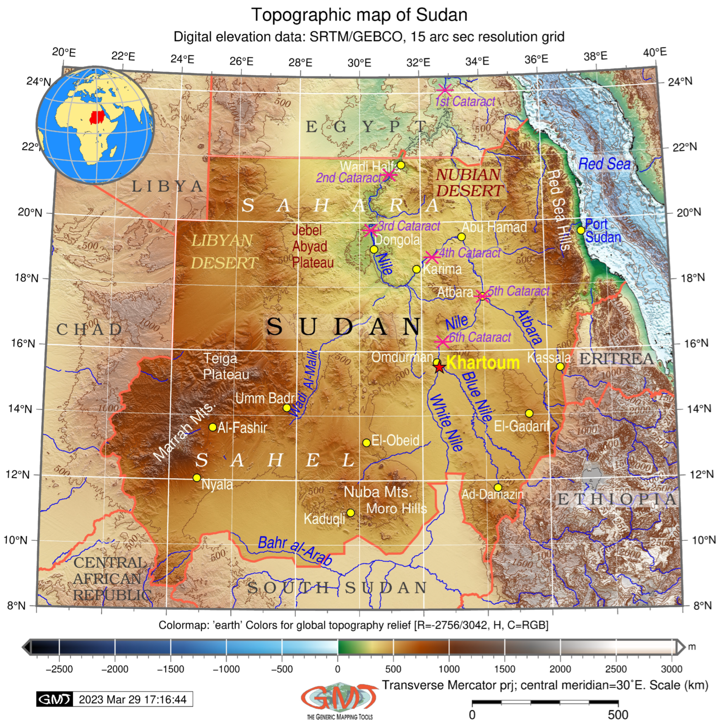
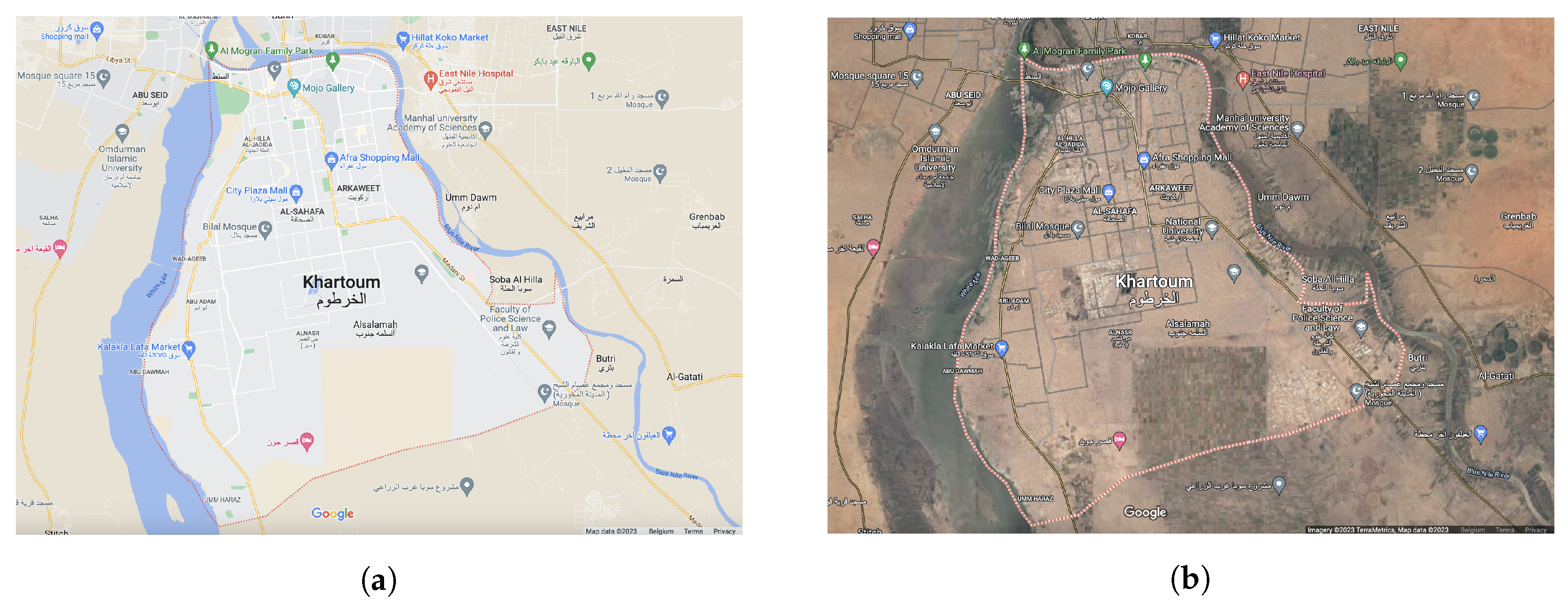
1.3. Study Area
2. Materials and Methods
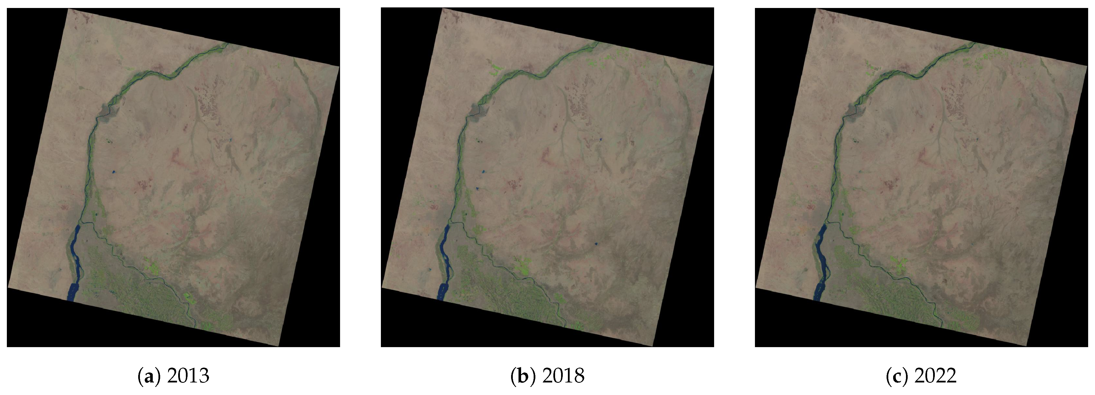
2.1. Data
2.2. Methodology
2.3. Calculating Vegetation Indices
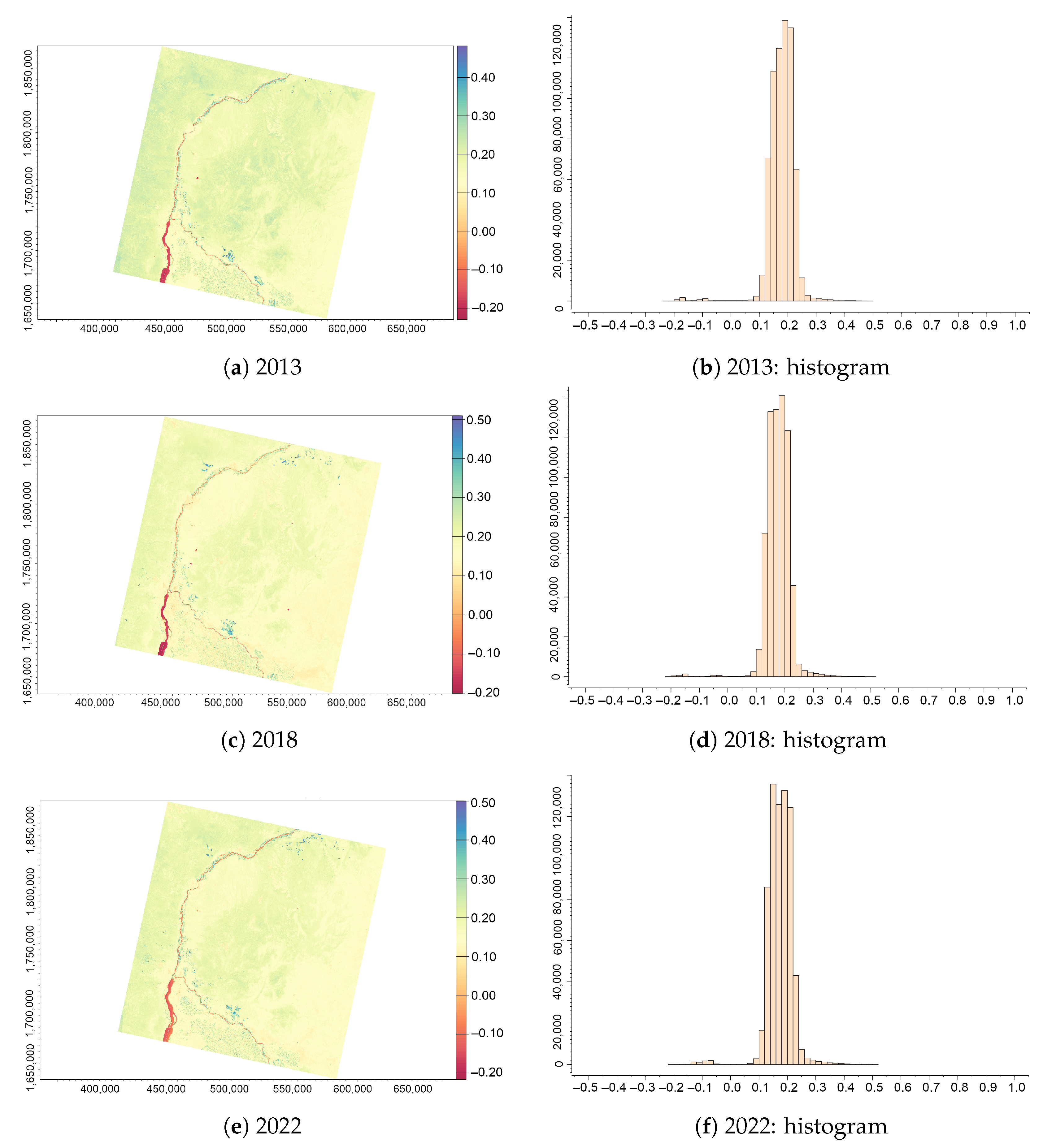
2.3.1. Normalised Difference Vegetation Index (NDVI)
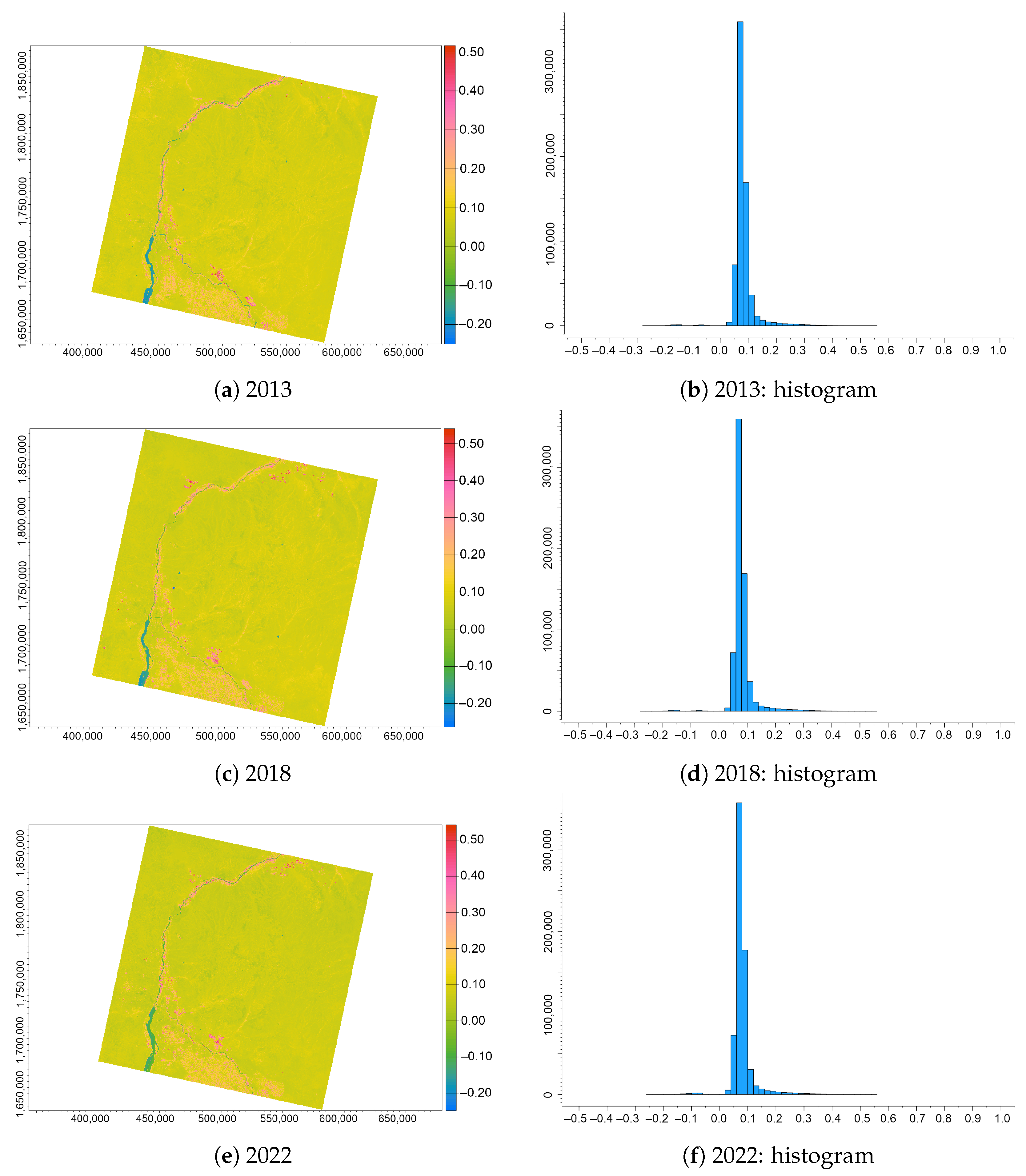
2.3.2. Green Normalised Difference Vegetation Index (GNDVI)
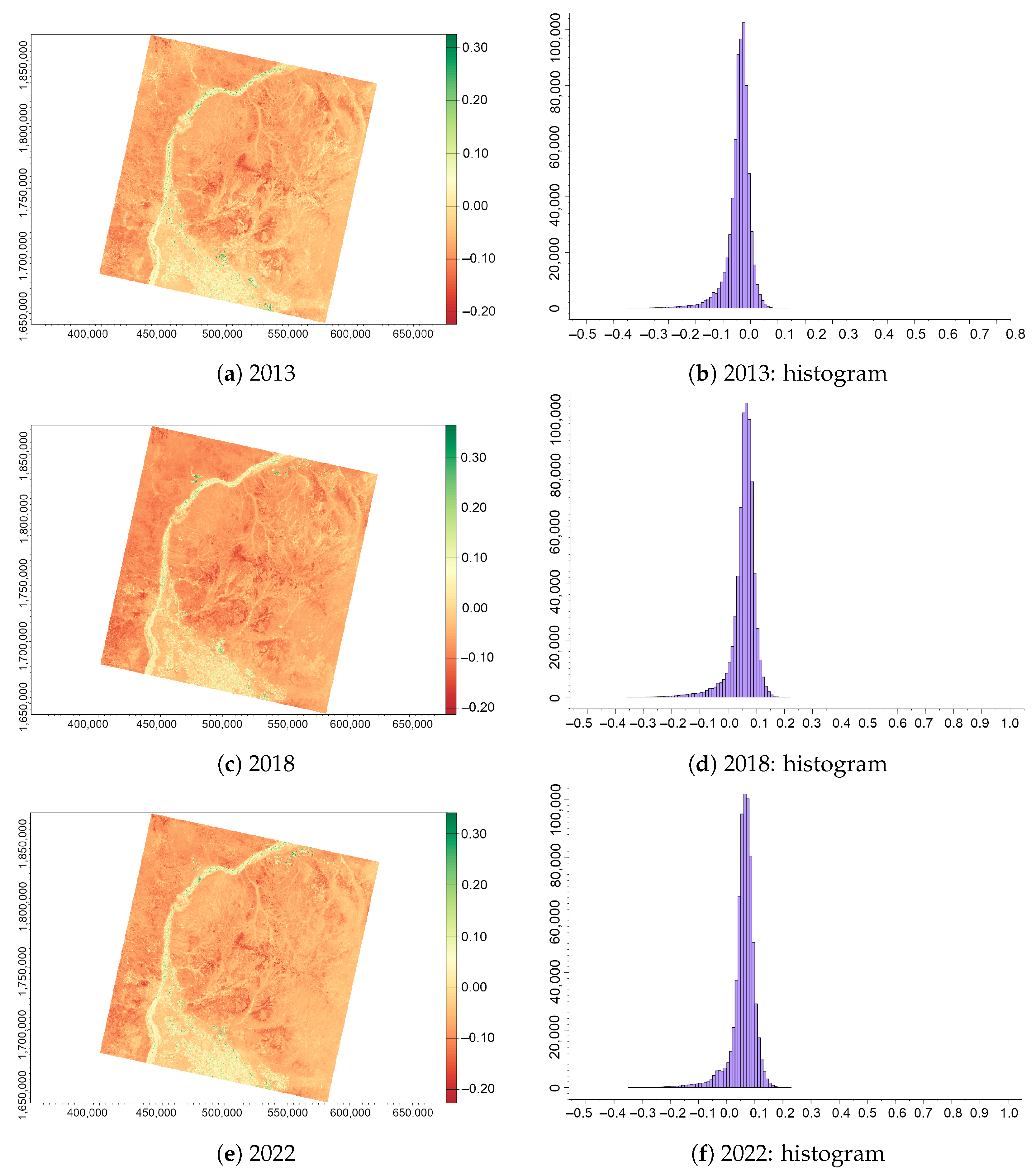
2.3.3. Normalised Difference Water Index (NDWI)
2.3.4. Optimised Soil-Adjusted Vegetation Index (OSAVI)
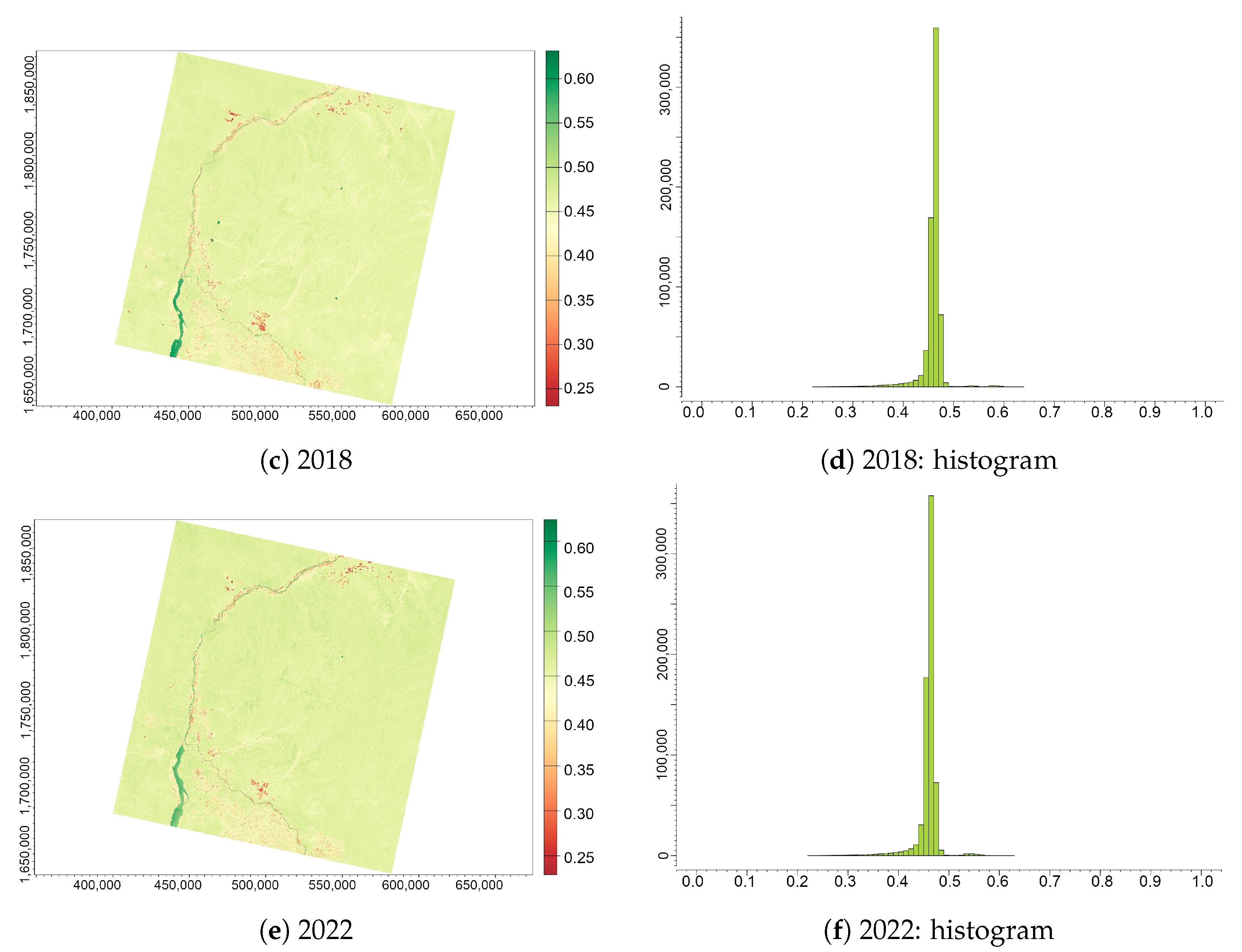
2.3.5. Infrared Percentage Vegetation Index (IPVI)
3. Results
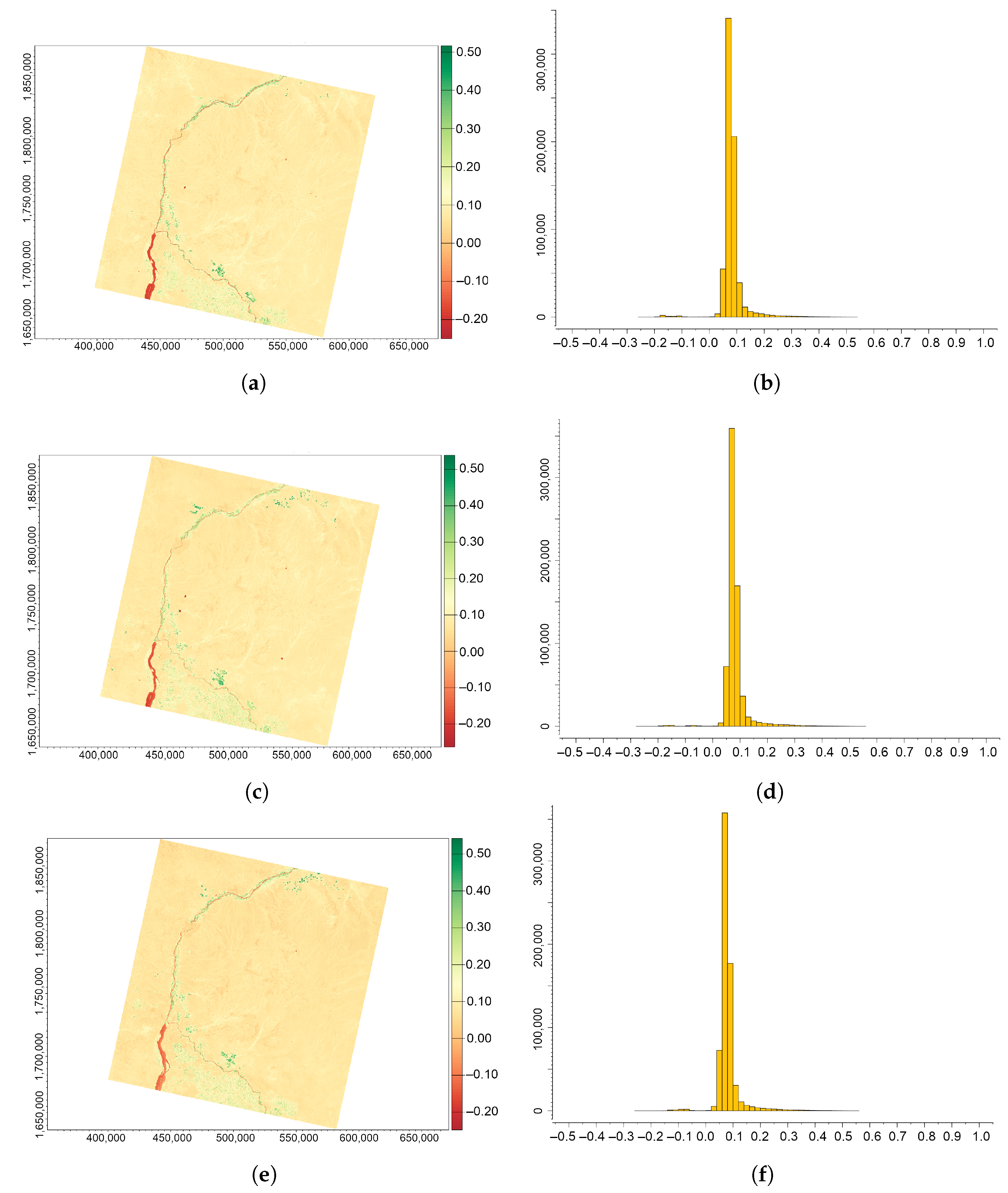
3.1. Normalised Difference Vegetation Index (NDVI)
3.2. Green Normalised Difference Vegetation Index (GNDVI)
3.3. Normalised Difference Water Index (NDWI)
3.4. Optimised Soil-Adjusted Vegetation Index (OSAVI)
3.5. Infrared Percentage Vegetation Index (IPVI)
4. Discussion
5. Conclusions
Author Contributions
Funding
Institutional Review Board Statement
Informed Consent Statement
Data Availability Statement
Acknowledgments
Conflicts of Interest
Abbreviations
| ENVI | ENvironment for Visualizing Images |
| ERDAS Imagine | Earth Resources Data Analysis System Imagine |
| GIS | Geographic Information System |
| GMT | Generic Mapping Tools |
| GNDVI | Green Normalised Difference Vegetation Index |
| IPVI | Infrared Percentage Vegetation Index |
| Landsat 8–9 OLI/TIRS | Landsat 8–9 Operational Land Imager (OLI) and Thermal Infrared (TIRS) |
| NDVI | Normalised Difference Vegetation Index |
| NDWI | Normalised Difference Water Index |
| OSAVI | Optimised Soil-Adjusted Vegetation Index |
| SAVI | Soil-Adjusted Vegetation Index |
| USGS | United States Geological Survey |
| UTM | Universal Transverse Mercator |
| VIs | Vegetation Indices |
| WGS84 | World Geodetic System 1984 |
Appendix A. Metadata on the Landsat 8–9 OLI/TIRS Images (USGS EarthExplorer)

| Dataset Attribute | Attributes for Image on 21 December 2018 | Attributes for 18 December 2018 | Attributes for 20 December 2018 |
|---|---|---|---|
| Landsat Scene Identifier | LC91730492022355LGN01 | LC81730492018352LGN00 | LC81730492013354LGN01 |
| Date Acquired | 21 December 2018 | 18 December 2018 | 20 December 2018 |
| Collection Category | T1 | T1 | T1 |
| Collection Number | 2 | 2 | 2 |
| WRS Path | 173 | 173 | 173 |
| WRS Row | 49 | 49 | 49 |
| Target WRS Path | 173 | 173 | 173 |
| Target WRS Row | 49 | 49 | 49 |
| Nadir/Off Nadir | NADIR | NADIR | NADIR |
| Roll Angle | −0.001 | 0.000 | 0.000 |
| Date Product Generated L2 | 17 March 2023 | 30 August 2020 | 12 September 2020 |
| Date Product Generated L1 | 17 March 2023 | 30 August 2020 | 12 September 2020 |
| Start Time | 21 December 2022 08:09:26 | 18 December 2018 08:08:54.736348 | 20 December 2013 08:10:29.988456 |
| Stop Time | 21 December 2022 08:09:58 | 18 December 2018 08:09:26.506347 | 20 December 2013 08:11:01.758452 |
| Station Identifier | LGN | LGN | LGN |
| Day/Night Indicator | DAY | DAY | DAY |
| Land Cloud Cover | 0.00 | 0.00 | 0.00 |
| Scene Cloud Cover L1 | 0.00 | 0.00 | 0.00 |
| Ground Control Points Model | 511 | 521 | 639 |
| Ground Control Points Version | 5 | 5 | 5 |
| Geometric RMSE Model | 7.263 | 6.387 | 4.378 |
| Geometric RMSE Model X | 5.055 | 4.612 | 2.951 |
| Geometric RMSE Model Y | 5.216 | 4.418 | 3.234 |
| Processing Software Version | LPGS_16.2.0 | LPGS_15.3.1c | LPGS_15.3.1c |
| Sun Elevation L0RA | 44.22152569 | 44.38827439 | 44.40055924 |
| Sun Azimuth L0RA | 148.68774152 | 148.91482828 | 149.05309430 |
| TIRS SSM Model | N/A | FINAL | ACTUAL |
| Data Type L2 | OLI_TIRS_L2SP | OLI_TIRS_L2SP | OLI_TIRS_L2SP |
| Sensor Identifier | OLI_TIRS | OLI_TIRS | OLI_TIRS |
| Satellite | 9 | 8 | 8 |
| Product Map Projection L1 | UTM | UTM | UTM |
| UTM Zone | 36 | 36 | 36 |
| Datum | WGS84 | WGS84 | WGS84 |
| Ellipsoid | WGS84 | WGS84 | WGS84 |
| Scene Center Lat DMS | 15°5403.06 N | 15°5403.56 N | 15°5403.42 N |
| Scene Center Long DMS | 33°0632.69 E | 33°0735.51 E | 33°0559.28 E |
| Corner Upper Left Lat DMS | 16°5634.84 N | 16°5644.88 N | 16°5644.41 N |
| Corner Upper Left Long DMS | 32°0224.68 E | 32°0325.49 E | 32°0144.08 E |
| Corner Upper Right Lat DMS | 16°5630.70 N | 16°5640.13 N | 16°5640.63 N |
| Corner Upper Right Long DMS | 34°1042.96 E | 34°1143.87 E | 34°1012.61 E |
| Corner Lower Left Lat DMS | 14°5038.76 N | 14°5039.01 N | 14°5038.58 N |
| Corner Lower Left Long DMS | 32°0300.32 E | 32°0400.55 E | 32°0220.18 E |
| Corner Lower Right Lat DMS | 14°5035.16 N | 14°5034.87 N | 14°5035.34 N |
| Corner Lower Right Long DMS | 34°0959.18 E | 34°1059.41 E | 34°0929.09 E |
| Scene Center Latitude | 15.90085 | 15.90099 | 15.90095 |
| Scene Center Longitude | 33.10908 | 33.12653 | 33.09980 |
| Corner Upper Left Latitude | 16.94301 | 16.94580 | 16.94567 |
| Corner Upper Left Longitude | 32.04019 | 32.05708 | 32.02891 |
| Corner Upper Right Latitude | 16.94186 | 16.94448 | 16.94462 |
| Corner Upper Right Longitude | 34.17860 | 34.19552 | 34.17017 |
| Corner Lower Left Latitude | 14.84410 | 14.84417 | 14.84405 |
| Corner Lower Left Longitude | 32.05009 | 32.06682 | 32.03894 |
| Corner Lower Right Latitude | 14.84310 | 14.84302 | 14.84315 |
| Corner Lower Right Longitude | 34.16644 | 34.18317 | 34.15808 |
Appendix B. R Scripts Used for Computing and Plotting the Vegetation Indices
Appendix B.1. R Code for Computing the NDVI
| Listing A1. R code for computing the NDVI (here: a case from 2022). |
 |
Appendix B.2. R Code for Computing the GNDVI
| Listing A2. R code for computing the GNDVI (here: a case from 2013). |
 |
Appendix B.3. R Code for Computing the NDWI
| Listing A3. R code for computing the NDWI (here: a case from 2018). |
 |
Appendix B.4. R Code for Computing the OSAVI
| Listing A4. R code for computing the OSAVI (here: a case from 2022). |
 |
Appendix B.5. R code for computing the IPVI
| Listing A5. R code for computing the IPVI (here: a case from 2013). |
 |
References
- Ahmed, S.A.; Kheiry, M.A.; Mofadel Hassan, I. 4—Impact of Vegetation Cover Changes on Gum Arabic Production Using Remote Sensing Applications in Gedarif State, Sudan. In Gum Arabic; Mariod, A.A., Ed.; Academic Press: Cambridge, MA, USA, 2018; pp. 29–43. [Google Scholar] [CrossRef]
- Hawash, E.; El-Hassanin, A.; Amer, W.; El-Nahry, A.; Effat, H. Change detection and urban expansion of Port Sudan, Red Sea, using remote sensing and GIS. Environ. Monit. Assess. 2021, 193, 723. [Google Scholar] [CrossRef] [PubMed]
- Youssef, A.M.; Ibrahem, S.M.; El Sayed, A.N.; Masoud, M.H. Assessment and management of water resources in Wadi El-Deeb using geophysical, hydrological and GIS techniques-Red Sea. J. Afr. Earth Sci. 2020, 164, 103777. [Google Scholar] [CrossRef]
- Qu, L.; Shao, Y.; Zhang, L. Land suitability evaluation method based on GIS technology. In Proceedings of the 2013 Second International Conference on Agro-Geoinformatics (Agro-Geoinformatics), Fairfax, VA, USA, 12–16 August 2013; pp. 7–12. [Google Scholar] [CrossRef]
- Aldoma, A.; Mohamed, M. Simulation of rainfall runoff process for Khartoum State (Sudan) using remote sensing and geographic information systems (GIS). Int. J. Water Resour. Environ. Eng. 2014, 6, 98–105. [Google Scholar]
- Abdekareem, M.; Al-Arifi, N.; Abdalla, F.; Mansour, A.; El-Baz, F. Fusion of Remote Sensing Data Using GIS-Based AHP-Weighted Overlay Techniques for Groundwater Sustainability in Arid Regions. Sustainability 2022, 14, 7871. [Google Scholar] [CrossRef]
- El Bastawesy, M.; Cherif, O.; Sultan, M. The geomorphological evidences of subsidence in the Nile Delta: Analysis of high resolution topographic DEM and multi-temporal satellite images. J. Afr. Earth Sci. 2017, 136, 252–261. [Google Scholar] [CrossRef]
- Sosnowski, A.; Ghoneim, E.; Burke, J.J.; Hines, E.; Halls, J. Remote regions, remote data: A spatial investigation of precipitation, dynamic land covers, and conflict in the Sudd wetland of South Sudan. Appl. Geogr. 2016, 69, 51–64. [Google Scholar] [CrossRef]
- Gorsevski, V.; Geores, M.; Kasischke, E. Human dimensions of land use and land cover change related to civil unrest in the Imatong Mountains of South Sudan. Appl. Geogr. 2013, 38, 64–75. [Google Scholar] [CrossRef]
- Wilson, E.H.; Sader, S.A. Detection of forest harvest type using multiple dates of Landsat TM imagery. Remote Sens. Environ. 2002, 80, 385–396. [Google Scholar] [CrossRef]
- Lemenkova, P.; Debeir, O. Satellite Image Processing by Python and R Using Landsat 9 OLI/TIRS and SRTM DEM Data on Côte d’Ivoire, West Africa. J. Imaging 2022, 8, 317. [Google Scholar] [CrossRef]
- Khiry, M.A.; Csaplovics, E. Appropriate Methods for Monitoring and Mapping Land Cover Changes in Semi-arid Areas in North Kordofan (Sudan) by Using Satellite Imagery and Spectral Mixture Analysis. In Proceedings of the 2007 International Workshop on the Analysis of Multi-temporal Remote Sensing Images, Leuven, Belgium, 18–20 July 2007; pp. 1–4. [Google Scholar] [CrossRef]
- Salih, A.A.; Ganawa, E.T.; Elmahl, A.A. Spectral mixture analysis (SMA) and change vector analysis (CVA) methods for monitoring and mapping land degradation/desertification in arid and semiarid areas (Sudan), using Landsat imagery. Egypt. J. Remote Sens. Space Sci. 2017, 20, S21–S29. [Google Scholar] [CrossRef]
- Nori, W.; Sulieman, H.M.; Niemeyer, I. Detection of land cover changes in El Rawashda Forest, Sudan: A systematic comparison. In Proceedings of the 2009 IEEE International Geoscience and Remote Sensing Symposium, Cape Town, South Africa, 12–17 July 2009; Volume 1, pp. 88–91. [Google Scholar] [CrossRef]
- Lemenkova, P.; Debeir, O. R Libraries for Remote Sensing Data Classification by k-means Clustering and NDVI Computation in Congo River Basin, DRC. Appl. Sci. 2022, 12, 12554. [Google Scholar] [CrossRef]
- Seaquist, J.; Chappell, A.; Eklundh, L. Exploring and improving NOAA AVHRR NDVI image quality for African drylands. In Proceedings of the IEEE International Geoscience and Remote Sensing Symposium, Toronto, ON, Canada, 24–28 June 2002; Volume 4, pp. 2006–2008. [Google Scholar] [CrossRef]
- Rivera-Marin, D.; Dash, J.; Ogutu, B. The use of remote sensing for desertification studies: A review. J. Arid Environ. 2022, 206, 104829. [Google Scholar] [CrossRef]
- Ali, R.; Zahran, S. Evaluation of NASA land information system in prediction stream runoff: Case study of Atbara and Blue Nile Sub-Basins. In Modeling Earth Systems and Environment; Springer: Cham, Switzerland, 2023. [Google Scholar] [CrossRef]
- Kumar, B.; Babu, K.; Anusha, B.; Rajasekhar, M. Geo-environmental monitoring and assessment of land degradation and desertification in the semi-arid regions using Landsat 8 OLI / TIRS, LST, and NDVI approach. Environ. Challenges 2022, 8, 100578. [Google Scholar] [CrossRef]
- Rashid, M.B.; Sheik, M.R.; Haque, A.E.; Siddique, M.A.B.; Habib, M.A.; Patwary, M.A.A. Salinity-induced change in green vegetation and land use patterns using remote sensing, NDVI, and GIS techniques: A case study on the southwestern coast of Bangladesh. Case Stud. Chem. Environ. Eng. 2023, 7, 100314. [Google Scholar] [CrossRef]
- Ezaidi, S.; Aydda, A.; Kabbachi, B.; Althuwaynee, O.F.; Ezaidi, A.; Haddou, M.A.; Idoumskine, I.; Thorpe, J.; Park, H.J.; Kim, S.W. Multi-temporal Landsat-derived NDVI for vegetation cover degradation for the period 1984-2018 in part of the Arganeraie Biosphere Reserve (Morocco). Remote Sens. Appl. Soc. Environ. 2022, 27, 100800. [Google Scholar] [CrossRef]
- de la Iglesia Martinez, A.; Labib, S. Demystifying normalized difference vegetation index (NDVI) for greenness exposure assessments and policy interventions in urban greening. Environ. Res. 2023, 220, 115155. [Google Scholar] [CrossRef]
- Omar, M.S.; Kawamukai, H. Prediction of NDVI using the Holt-Winters model in high and low vegetation regions: A case study of East Africa. Sci. Afr. 2021, 14, e01020. [Google Scholar] [CrossRef]
- Wang, C.; Wang, A.; Guo, D.; Li, H.; Zang, S. Off-peak NDVI correction to reconstruct Landsat time series for post-fire recovery in high-latitude forests. Int. J. Appl. Earth Obs. Geoinf. 2022, 107, 102704. [Google Scholar] [CrossRef]
- Barriguinha, A.; Jardim, B.; de Castro Neto, M.; Gil, A. Using NDVI, climate data and machine learning to estimate yield in the Douro wine region. Int. J. Appl. Earth Obs. Geoinf. 2022, 114, 103069. [Google Scholar] [CrossRef]
- Roy, B. Optimum machine learning algorithm selection for forecasting vegetation indices: MODIS NDVI & EVI. Remote Sens. Appl. Soc. Environ. 2021, 23, 100582. [Google Scholar] [CrossRef]
- Li, J.; Li, C.; Xu, W.; Feng, H.; Zhao, F.; Long, H.; Meng, Y.; Chen, W.; Yang, H.; Yang, G. Fusion of optical and SAR images based on deep learning to reconstruct vegetation NDVI time series in cloud-prone regions. Int. J. Appl. Earth Obs. Geoinf. 2022, 112, 102818. [Google Scholar] [CrossRef]
- Davidson, C.; Jaganathan, V.; Sivakumar, A.N.; Czarnecki, J.M.P.; Chowdhary, G. NDVI/NDRE prediction from standard RGB aerial imagery using deep learning. Comput. Electron. Agric. 2022, 203, 107396. [Google Scholar] [CrossRef]
- Zhao, J.; Wang, Y.; Zhang, H. Automated batch processing of mass remote sensing and geospatial data to meet the needs of end users. In Proceedings of the 2011 IEEE International Geoscience and Remote Sensing Symposium, Vancouver, BC, Canada, 24–29 July 2011; pp. 3464–3467. [Google Scholar] [CrossRef]
- Lemenkova, P.; Debeir, O. Quantitative Morphometric 3D Terrain Analysis of Japan Using Scripts of GMT and R. Land 2023, 12, 261. [Google Scholar] [CrossRef]
- Zhang, M.; Yue, P.; Guo, X. GIScript: Towards an interoperable geospatial scripting language for GIS programming. In Proceedings of the 2014 The Third International Conference on Agro-Geoinformatics, Beijing, China, 11–14 August 2014; pp. 1–5. [Google Scholar] [CrossRef]
- Lemenkova, P.; Debeir, O. Seismotectonics of Shallow-Focus Earthquakes in Venezuela with Links to Gravity Anomalies and Geologic Heterogeneity Mapped by a GMT Scripting Language. Sustainability 2022, 14, 15966. [Google Scholar] [CrossRef]
- Pandit, A.; Sawant, S.; Mohite, J.; Pappula, S. Development of Geospatial Processing Frameworks for Sentinel-1, -2 Satellite Data. In Proceedings of the IGARSS 2020–2020 IEEE International Geoscience and Remote Sensing Symposium, Waikoloa, HI, USA, 26 September–2 October 2020; pp. 3123–3126. [Google Scholar] [CrossRef]
- Walter, G.; Warmerdam, F.; Farris-Manning, P. An open source tool for geospatial image exploitation. In Proceedings of the IEEE International Geoscience and Remote Sensing Symposium, Toronto, ON, Canada, 24–28 June 2002; Volume 6, pp. 3522–3524. [Google Scholar] [CrossRef]
- Leveau, L.M.; Isla, F.I. Predicting bird species presence in urban areas with NDVI: An assessment within and between cities. Urban For. Urban Green. 2021, 63, 127199. [Google Scholar] [CrossRef]
- Chávez, R.O.; Meseguer-Ruiz, O.; Olea, M.; Calderón-Seguel, M.; Yager, K.; Isela Meneses, R.; Lastra, J.A.; Núñez-Hidalgo, I.; Sarricolea, P.; Serrano-Notivoli, R.; et al. Andean peatlands at risk? Spatiotemporal patterns of extreme NDVI anomalies, water extraction and drought severity in a large-scale mining area of Atacama, northern Chile. Int. J. Appl. Earth Obs. Geoinf. 2023, 116, 103138. [Google Scholar] [CrossRef]
- Klimavičius, L.; Rimkus, E.; Stonevičius, E.; Mačiulytė, V. Seasonality and long-term trends of NDVI values in different land use types in the eastern part of the Baltic Sea basin. Oceanologia 2023, 65, 171–181. [Google Scholar] [CrossRef]
- Prăvălie, R.; Sîrodoev, I.; Nita, I.A.; Patriche, C.; Dumitraşcu, M.; Roşca, B.; Tişcovschi, A.; Bandoc, G.; Săvulescu, I.; Mănoiu, V.; et al. NDVI-based ecological dynamics of forest vegetation and its relationship to climate change in Romania during 1987–2018. Ecol. Indic. 2022, 136, 108629. [Google Scholar] [CrossRef]
- Alvi, S.H. Climatic changes, desertification and the Republic of Sudan. GeoJournal 1994, 33, 393–399. [Google Scholar] [CrossRef]
- Dawelbait, M.; Morari, F. Monitoring desertification in a Savannah region in Sudan using Landsat images and spectral mixture analysis. J. Arid Environ. 2012, 80, 45–55. [Google Scholar] [CrossRef]
- Mohamed, M.A.; El Afandi, G.S.; El-Mahdy, M.E.S. Impact of climate change on rainfall variability in the Blue Nile basin. Alex. Eng. J. 2022, 61, 3265–3275. [Google Scholar] [CrossRef]
- Hulme, M. The adaptability of a rural water supply system to extreme rainfall anomalies in central Sudan. Appl. Geogr. 1986, 6, 89–105. [Google Scholar] [CrossRef]
- Elagib, N.A. Changing rainfall, seasonality and erosivity in the hyper-arid zone of Sudan. Land Degrad. Dev. 2011, 22, 505–512. [Google Scholar] [CrossRef]
- Ayoub, A.T. Land degradation, rainfall variability and food production in the Sahelian zone of the Sudan. Land Degrad. Dev. 1999, 10, 489–500. [Google Scholar] [CrossRef]
- Akhtar, M.; Mensching, H.; Domnick, I. Methods applied for recording desertification and their results from Sahel region of the Republic of Sudan. Desertif. Control Bull. 1994, 25, 40–47. [Google Scholar]
- Salih, A.A.; Hamid, A.A. Hydrological studies in the White Nile State in Sudan. Egypt. J. Remote Sens. Space Sci. 2017, 20, S31–S38. [Google Scholar] [CrossRef]
- Fuller, T.D. Resettlement as a desertification control measure: A case study in Darfur Region, Sudan—Part II: Recommendations. Agric. Adm. Ext. 1987, 26, 39–55. [Google Scholar] [CrossRef]
- Salih, A.; Hassaballa, A.A. Quantitative Assessment of Land Sensitivity to Desertification in Central Sudan: An Application of Remote Sensing-Based MEDALUS Model. In Applications of Space Techniques on the Natural Hazards in the MENA Region; Springer International Publishing: Cham, Switzerland, 2022; pp. 419–446. [Google Scholar] [CrossRef]
- Tariku, T.B.; Gan, K.E.; Tan, X.; Gan, T.Y.; Shi, H.; Tilmant, A. Global warming impact to River Basin of Blue Nile and the optimum operation of its multi-reservoir system for hydropower production and irrigation. Sci. Total Environ. 2021, 767, 144863. [Google Scholar] [CrossRef]
- Sulieman, H.; Elagib, N. Implications of climate, land-use and land-cover changes for pastoralism in eastern Sudan. J. Arid Environ. 2012, 85, 132–141. [Google Scholar] [CrossRef]
- Wessel, P.; Luis, J.F.; Uieda, L.; Scharroo, R.; Wobbe, F.; Smith, W.H.F.; Tian, D. The Generic Mapping Tools Version 6. Geochem. Geophys. Geosyst. 2019, 20, 5556–5564. [Google Scholar] [CrossRef]
- El-Karouri, M.O.H. The Impact of Desertification on Land Productivity in Sudan. In Physics of Desertification; Springer: Dordrecht, The Netherlands, 1986; pp. 52–58. [Google Scholar] [CrossRef]
- Pearce, D. Natural resource management and anti-desertification policy in the Sahel-Sudan zone: A case study of Gum Arabic. GeoJournal 1988, 17, 349–355. [Google Scholar] [CrossRef]
- Yang, Z.; Gao, X.; Lei, J.; Meng, X.; Zhou, N. Analysis of spatiotemporal changes and driving factors of desertification in the Africa Sahel. CATENA 2022, 213, 106213. [Google Scholar] [CrossRef]
- Falkenmark, M.; Rockström, J. Building resilience to drought in desertification-prone savannas in Sub-Saharan Africa: The water perspective. Nat. Resour. Forum 2008, 32, 93–102. [Google Scholar] [CrossRef]
- Khiry, M.; Dafalla, M.; Csaplovics, E. Mapping and assessment of sand encroachment by spectral mixture analysis in arid and semi-arid areas: Case study North Kordofan, Sudan. In Proceedings of the 6th International Conference on “Earth Observation & Geoinformation Sciences in Support of Africa’s Development” (AARSE2006), Cairo, Egypt, 30 October–2 November 2006; pp. 1–7. [Google Scholar]
- Shamim, M.Z.M.; Elsheikh, E.A.A.; Salih, F.E.M.S.; Islam, M.R. Signal Attenuation Prediction Model for a 22 GHz Terrestrial Communication Link in Sudan Due to Dust and Sand Storms Using Machine Learning. IEEE Access 2021, 9, 164632–164642. [Google Scholar] [CrossRef]
- Elsheikh, E.A.A.; Islam, M.R.; Habaebi, M.H.; Ismail, A.F.; Zyoud, A. Dust Storm Attenuation Modeling Based on Measurements in Sudan. IEEE Trans. Antennas Propag. 2017, 65, 4200–4208. [Google Scholar] [CrossRef]
- Elsheikh, E.A.A.; Rafiqul, I.M.; Ismail, A.F.; Habaebi, M.; Chebil, J. Dust storms attenuation measurements at 14 GHz and 21 GHz in Sudan. In Proceedings of the 2015 International Conference on Computing, Control, Networking, Electronics and Embedded Systems Engineering (ICCNEEE), Khartoum, Sudan, 7–9 September 2015; pp. 11–16. [Google Scholar] [CrossRef]
- Biro, K.; Pradhan, B.; Buchroithner, M.; Makeschin, F. Land Use/Land Cover Change Analysis and its Impact on Soil Properties in the Northern Part of Gadarif Region, Sudan. Land Degrad. Dev. 2013, 24, 90–102. [Google Scholar] [CrossRef]
- El-Niweiri, M.A.A.; Moritz, R.F.A.; Lattorff, H.M.G. The Invasion of the Dwarf Honeybee, Apis florea, along the River Nile in Sudan. Insects 2019, 10, 405. [Google Scholar] [CrossRef]
- Fuller, D.; Parenti, M.; Hassan, A.; Beier, J.C. Linking land cover and species distribution models to project potential ranges of malaria vectors: An example using Anopheles arabiensis in Sudan and Upper Egypt. Malar. J. 2012, 11, 264. [Google Scholar] [CrossRef]
- Melesse, A.M.; Abtew, W.; Setegn, S.G. Nile River Basin, 1st ed.; Ecohydrological Challenges, Climate Change and Hydropolitics; Springer: Cham, Switzerland, 2016. [Google Scholar]
- Hamad, O.; El-Battahani, A. Sudan and the Nile Basin. Aquat. Sci. 2005, 67, 28–41. [Google Scholar] [CrossRef]
- Halwagy, R. Studies on the succession of vegetation on some islands and sand banks in the nile near Khartoum, Sudan. Vegetatio 1963, 11, 217–234. [Google Scholar] [CrossRef]
- Billi, P.; el Badri Ali, O. Sediment transport of the Blue Nile at Khartoum. Quat. Int. 2010, 226, 12–22. [Google Scholar] [CrossRef]
- Pacini, N.; Harper, D.M. Hydrological characteristics and water resources management in the Nile Basin. Ecohydrol. Hydrobiol. 2016, 16, 242–254. [Google Scholar] [CrossRef]
- Ayik, A.; Ijumba, N.; Kabiri, C.; Goffin, P. Preliminary assessment of small hydropower potential using the Soil and Water Assessment Tool model: A case study of Central Equatoria State, South Sudan. Energy Rep. 2023, 9, 2229–2246. [Google Scholar] [CrossRef]
- Kau, A.; Gramlich, R.; Sewilam, H. Modelling land suitability to evaluate the potential for irrigated agriculture in the Nile region in Sudan. Sustain. Water Resour. Manag. 2023, 9, 10. [Google Scholar] [CrossRef]
- Kobayashi, A. Desertification. In International Encyclopedia of Human Geography, 2nd ed.; Kobayashi, A., Ed.; Elsevier: Oxford, UK, 2020; pp. 257–262. [Google Scholar] [CrossRef]
- Sulieman, H.M. Expansion of mechanized rain-fed agriculture and land-use/land-cover change in the Southern Gadarif, Sudan. Afr. J. Agric. Res. 2010, 5, 1609–1615. [Google Scholar]
- Ibrahim, F. Anthropogenic causes of desertification in Western Sudan. GeoJournal 1978, 2, 243–254. [Google Scholar] [CrossRef]
- Ahmed, S.M. Impacts of drought, food security policy and climate change on performance of irrigation schemes in Sub-saharan Africa: The case of Sudan. Agric. Water Manag. 2020, 232, 106064. [Google Scholar] [CrossRef]
- Nesser, G.; Abdelbagi, A.; Ishag, A.; Hammad, A.M.A.; Tagelseed, M. Seasonal levels of pesticide residues in the main and the Blue Nile waters in Sudan. Arab. J. Geosci. 2020, 13, 994. [Google Scholar] [CrossRef]
- Ahmed, A. Land use history of Jebel Marra, Sudan, as related to the present distribution of woody vegetation. GeoJournal 1982, 6, 5–14. [Google Scholar] [CrossRef]
- Sulieman, H.; Ahmed, A. Monitoring changes in pastoral resources in eastern Sudan: A synthesis of remote sensing and local knowledge. Pastoralism 2013, 3, 22. [Google Scholar] [CrossRef]
- Akhtar, M.; Mensching, H. Desertification in the Butana. GeoJournal 1993, 31, 41–50. [Google Scholar] [CrossRef]
- Schumacher, J.; Luedeling, E.; Gebauer, J.; Saied, A.; El-Siddig, K.; Buerkert, A. Spatial expansion and water requirements of urban agriculture in Khartoum, Sudan. J. Arid Environ. 2009, 73, 399–406. [Google Scholar] [CrossRef]
- Babiker, A. Urbanization and desertification in the Sudan with special reference to Khartoum. GeoJournal 1982, 6, 69–76. [Google Scholar] [CrossRef]
- Mohammed, E.; Alawad, H.; Zeinelabdein, K.; Ali, A. Urban expansion and population growth in Omdurman city, Sudan using geospatial technologies and statistical approaches. Am. J. Earth Sci. 2015, 2, 1–7. [Google Scholar]
- Sasmaz, A. The Atbara porphyry gold–copper systems in the Red Sea Hills, Neoproterozoic Arabian–Nubian Shield, NE Sudan. J. Geochem. Explor. 2020, 214, 106539. [Google Scholar] [CrossRef]
- Khiry, M.A. Spectral Mixture Analysis for Monitoring and Mapping Desertification Processes in Semi-Arid Areas in North Kordofan State, Sudan; University of Dresden: Dresden, Germany, 2007. [Google Scholar] [CrossRef]
- Elnashar, A.; Zeng, H.; Wu, B.; Gebremicael, T.G.; Marie, K. Assessment of environmentally sensitive areas to desertification in the Blue Nile Basin driven by the MEDALUS-GEE framework. Sci. Total Environ. 2022, 815, 152925. [Google Scholar] [CrossRef]
- Subramaniam, M.; Bunka, C.; Park, S.S. Desertification. In The Wiley-Blackwell Encyclopedia of Globalization; John Wiley & Sons, Ltd.: Hoboken, NJ, USA, 2013; pp. 1–10. [Google Scholar] [CrossRef]
- Honegger, M.; Williams, M. Human occupations and environmental changes in the Nile valley during the Holocene: The case of Kerma in Upper Nubia (northern Sudan). Quat. Sci. Rev. 2015, 130, 141–154. [Google Scholar] [CrossRef]
- Omar, A.; Abdi, E.K.; Glover, O.L. Causes and Impacts of Land Degradation and Desertification: Case Study of the Sudan. Int. J. Agric. For. 2013, 3, 40–51. [Google Scholar]
- Khalifa, M.; Elagib, N.A.; Ribbe, L.; Schneider, K. Spatio-temporal variations in climate, primary productivity and efficiency of water and carbon use of the land cover types in Sudan and Ethiopia. Sci. Total Environ. 2018, 624, 790–806. [Google Scholar] [CrossRef]
- Jahelnabi, A.; Zhao, J.; Li, C.; Fadoul, S.M.; Shi, Y.; Bsheer, A.K.; Yagoub, Y.E. Assessment of the contribution of climate change and human activities to desertification in Northern Kordofan-Province, Sudan using net primary productivity as an indicator. Contemp. Probl. Ecol. 2016, 9, 674–683. [Google Scholar] [CrossRef]
- Darkoh, M.B.K. The nature, causes and consequences of desertification in the drylands of Africa. Land Degrad. Dev. 1998, 9, 1–20. [Google Scholar] [CrossRef]
- Conway, D. From headwater tributaries to international river: Observing and adapting to climate variability and change in the Nile basin. Glob. Environ. Chang. 2005, 15, 99–114. [Google Scholar] [CrossRef]
- Babiker, I.S.; Mohamed, M.A.A. Use of NRCS-curve number method for peak discharge estimation in Sharqu ElNeil locality, Khartoum, Sudan. Arab. J. Geosci. 2019, 12, 541. [Google Scholar] [CrossRef]
- Abdelmalik, K.W.; Abdelmohsen, K. GRACE and TRMM mission: The role of remote sensing techniques for monitoring spatio-temporal change in total water mass, Nile basin. J. Afr. Earth Sci. 2019, 160, 103596. [Google Scholar] [CrossRef]
- Elsheikh, A.; Abdelsalam, M.G.; Mickus, K. Geology and geophysics of the West Nubian Paleolake and the Northern Darfur Megalake (WNPL–NDML): Implication for groundwater resources in Darfur, northwestern Sudan. J. Afr. Earth Sci. 2011, 61, 82–93. [Google Scholar] [CrossRef]
- Mahmoud, A.; Obeid, M. Ecological studies in the vegetation of the Sudan. Plant Ecol. 1971, 23, 153–176. [Google Scholar] [CrossRef]
- Sene, K.; Tate, E.; Farquharson, F. Sensitivity Studies of the Impacts of Climate Change on White Nile Flows. Clim. Chang. 2001, 50, 177–208. [Google Scholar] [CrossRef]
- Bakhit, A.; Ibrahim, F. Geomorphological aspects of the process of desertification in Western Sudan. GeoJournal 1982, 6, 19–24. [Google Scholar] [CrossRef]
- Mohamed Ali, O.M. From vision to action: Towards a national policy for integrated water management in Sudan. In Water Resources Perspectives: Evaluation, Management and Policy; Developments in Water Science; Alsharhan, A.S., Wood, W.W., Eds.; Elsevier: Amsterdam, The Netherlands, 2003; Volume 50, pp. 237–244. [Google Scholar] [CrossRef]
- Elshaikh, A.E.; Yang, S.H.; Jiao, X.; Elbashier, M.M. Impacts of Legal and Institutional Changes on Irrigation Management Performance: A Case of the Gezira Irrigation Scheme, Sudan. Water 2018, 10, 1579. [Google Scholar] [CrossRef]
- Roy, D.; Kovalskyy, V.; Zhang, H.; Vermote, E.; Yan, L.; Kumar, S.; Egorov, A. Characterization of Landsat-7 to Landsat-8 reflective wavelength and normalized difference vegetation index continuity. Remote Sens. Environ. 2016, 185, 57–70. [Google Scholar] [CrossRef]
- Hammad, M.; Mucsi, L.; van Leeuwen, B. Land Cover Change Investigation in the Southern Syrian Coastal Basins During the Past 30-Years Using Landsat Remote Sensing Data. J. Environ. Geogr. 2018, 11, 45–51. [Google Scholar] [CrossRef]
- Liang, Y.; Yin, F.; Xie, D.; Liu, L.; Zhang, Y.; Ashraf, T. Inversion and Monitoring of the TP Concentration in Taihu Lake Using the Landsat-8 and Sentinel-2 Images. Remote Sens. 2022, 14, 6284. [Google Scholar] [CrossRef]
- Talebi, H.; Samadianfard, S.; Kamran, K.V. A novel method based on Landsat 8 and MODIS satellite images to estimate monthly reference evapotranspiration in arid and semi-arid climats. Water Soil Manag. Model. 2023, 3, 180–195. [Google Scholar] [CrossRef]
- Wang, J.; Xiao, X.; Qin, Y.; Dong, J.; Zhang, G.; Yang, X.; Wu, X.; Biradar, C.; Hu, Y. Annual forest maps in the contiguous United States during 2015–2017 from analyses of PALSAR-2 and Landsat images. Earth Syst. Sci. Data Discuss. 2023, 2023, 1–29. [Google Scholar] [CrossRef]
- Yilmaz, O.S.; Gulgen, F.; Balik Sanli, F.; Ates, A.M. The Performance Analysis of Different Water Indices and Algorithms Using Sentinel-2 and Landsat-8 Images in Determining Water Surface: Demirkopru Dam Case Study. Arab. J. Sci. Eng. 2023. [Google Scholar] [CrossRef]
- Nasseri, S.; Farhadi Bansouleh, B.; Azari, A. Estimation of land surface temperature in agricultural lands using Sentinel 2 images: A case study for sunflower fields. Irrig. Drain. 2023, 72, 1–11. [Google Scholar] [CrossRef]
- Li, R.; Wang, L.; Lu, Y. A comparative study on intra-annual classification of invasive saltcedar with Landsat 8 and Landsat 9. Int. J. Remote Sens. 2023, 44, 2093–2114. [Google Scholar] [CrossRef]
- Veretekhina, S.; Sergey, K.; Pronkina, T.; Khalyukin, V.; Alla, M.; Khudyakova, E.; Stepantsevich, M. Comparative Analysis of Big Data Acquisition Technology from Landsat 8 and Sentinel-2 Satellites. In Proceedings of the Cybernetics Perspectives in Systems; Silhavy, R., Ed.; Springer: Cham, Switzerland, 2022; pp. 41–53. [Google Scholar]
- Gumma, M.K.; Thenkabail, P.S.; Teluguntla, P.G.; Oliphant, A.; Xiong, J.; Giri, C.; Pyla, V.; Dixit, S.; Whitbread, A.M. Agricultural cropland extent and areas of South Asia derived using Landsat satellite 30-m time-series big-data using random forest machine learning algorithms on the Google Earth Engine cloud. GIScience Remote Sens. 2020, 57, 302–322. [Google Scholar] [CrossRef]
- Earth Resources Observation and Science (EROS) Center. Collection 2 Landsat 8–9 OLI (Operational Land Imager) and TIRS (Thermal Infrared Sensor) Level-2 Science Product. Online. Dataset. 2020. Available online: https://www.usgs.gov/centers/eros/science/usgs-eros-archive-landsat-archives-landsat-8-9-olitirs-collection-2-level-2 (accessed on 20 February 2023). [CrossRef]
- R Core Team. R: A Language and Environment for Statistical Computing; R Foundation for Statistical Computing: Vienna, Austria, 2022. [Google Scholar]
- Neuwirth, E. Package ‘RColorBrewer’. Version 1.1-3. 2022. Available online: https://cran.r-project.org/web/packages/RColorBrewer/index.html (accessed on 10 February 2023).
- Harrell, F.E., Jr. Hmisc: Harrell Miscellaneous. Version: 5.0-1. 2023. Available online: https://hbiostat.org/R/Hmisc/ (accessed on 15 February 2023).
- Wright, K. Pals. License GPL-3. 2021. Available online: https://kwstat.github.io/pals/ (accessed on 17 February 2023).
- Rouse, J.; Haas, R.; Scheel, J.; Deering, D. Monitoring Vegetation Systems in the Great Plains with ERTS. In Proceedings of the 3rd Earth Resource Technology Satellite (ERTS) Symposium, NASA. Goddard Space Flight Center 3d ERTS-1 Symp., Washington, DC, USA, 10–14 December 1974; Section A. Volume 1, pp. 48–62. [Google Scholar]
- Gwapedza, D.; Hughes, D.A.; Slaughter, A.R.; Mantel, S.K. Temporal Influences of Vegetation Cover (C) Dynamism on MUSLE Sediment Yield Estimates: NDVI Evaluation. Water 2021, 13, 2707. [Google Scholar] [CrossRef]
- Wu, S.; Gao, X.; Lei, J.; Zhou, N.; Wang, Y. Spatial and Temporal Changes in the Normalized Difference Vegetation Index and Their Driving Factors in the Desert/Grassland Biome Transition Zone of the Sahel Region of Africa. Remote Sens. 2020, 12, 4119. [Google Scholar] [CrossRef]
- Ghebrezgabher, M.G.; Yang, T.; Yang, X.; Eyassu Sereke, T. Assessment of NDVI variations in responses to climate change in the Horn of Africa. Egypt. J. Remote Sens. Space Sci. 2020, 23, 249–261. [Google Scholar] [CrossRef]
- Rulinda, C.; Dilo, A.; Bijker, W.; Stein, A. Characterising and quantifying vegetative drought in East Africa using fuzzy modelling and NDVI data. J. Arid Environ. 2012, 78, 169–178. [Google Scholar] [CrossRef]
- Gitelson, A.A.; Kaufman, Y.J.; Merzlyak, M.N. Use of a green channel in remote sensing of global vegetation from EOS-MODIS. Remote Sens. Environ. 1996, 58, 289–298. [Google Scholar] [CrossRef]
- Gao, B. NDWI – A normalized difference water index for remote sensing of vegetation liquid water from space. Remote Sens. Environ. 1996, 58, 257–266. [Google Scholar] [CrossRef]
- McFeeters, S.K. Using the Normalized Difference Water Index (NDWI) within a Geographic Information System to Detect Swimming Pools for Mosquito Abatement: A Practical Approach. Remote Sens. 2013, 5, 3544–3561. [Google Scholar] [CrossRef]
- Zheng, Y.; Tang, L.; Wang, H. An improved approach for monitoring urban built-up areas by combining NPP-VIIRS nighttime light, NDVI, NDWI, and NDBI. J. Clean. Prod. 2021, 328, 129488. [Google Scholar] [CrossRef]
- Teng, J.; Xia, S.; Liu, Y.; Yu, X.; Duan, H.; Xiao, H.; Zhao, C. Assessing habitat suitability for wintering geese by using Normalized Difference Water Index (NDWI) in a large floodplain wetland, China. Ecol. Indic. 2021, 122, 107260. [Google Scholar] [CrossRef]
- Rondeaux, G.; Steven, M.; Baret, F. Optimization of Soil-Adjusted Vegetation Indices. Remote Sens. Environ. 1996, 55, 95–107. [Google Scholar] [CrossRef]
- Crippen, R.E. Calculating the vegetation index faster. Remote Sens. Environ. 1990, 34, 71–73. [Google Scholar] [CrossRef]
- RStudio Team. RStudio, PBC. In RStudio: Integrated Development for R; RStudio, Inc.: Boston, MA, USA, 2020; Available online: http://www.rstudio.com/ (accessed on 28 March 2023).
- Dictionary. Biology Online. 2023. Available online: https://www.biologyonline.com/dictionary/vigor (accessed on 10 April 2023).


| Date | Spacecraft | Landsat Product ID | Scene ID |
|---|---|---|---|
| 20 December 2013 | Lands. 8 | LC08_L2SP_173049_20131220_20200912_02_T1 | LC81730492013354LGN01 |
| 18 December 2013 | Lands. 8 | LC08_L2SP_173049_20181218_20200830_02_T1 | LC81730492018352LGN00 |
| 21 December 2013 | Lands. 9 | LC09_L2SP_173049_20221221_20221224_02_T1 | LC91730492022355LGN00 |
| VI | 2013 | 2018 | 2022 |
|---|---|---|---|
| −0.2742168 | −0.2817099 | −0.2791084 | |
| 0.7246868 | 0.5796811 | 0.6044010 | |
| −0.2387020 | −0.2830099 | −0.2253696 | |
| 0.6371941 | 0.5690726 | 0.7235179 | |
| −0.4046338 | −0.5656914 | −0.5743572 | |
| 0.3880472 | 0.3764042 | 0.4152763 | |
| −0.2742153 | −0.2817084 | −0.2791067 | |
| 0.7246833 | 0.5796785 | 0.6043976 | |
| 0.1376566 | 0.2101595 | 0.1977995 | |
| 0.6371084 | 0.6408550 | 0.6395542 |
Disclaimer/Publisher’s Note: The statements, opinions and data contained in all publications are solely those of the individual author(s) and contributor(s) and not of MDPI and/or the editor(s). MDPI and/or the editor(s) disclaim responsibility for any injury to people or property resulting from any ideas, methods, instructions or products referred to in the content. |
© 2023 by the authors. Licensee MDPI, Basel, Switzerland. This article is an open access article distributed under the terms and conditions of the Creative Commons Attribution (CC BY) license (https://creativecommons.org/licenses/by/4.0/).
Share and Cite
Lemenkova, P.; Debeir, O. Multispectral Satellite Image Analysis for Computing Vegetation Indices by R in the Khartoum Region of Sudan, Northeast Africa. J. Imaging 2023, 9, 98. https://doi.org/10.3390/jimaging9050098
Lemenkova P, Debeir O. Multispectral Satellite Image Analysis for Computing Vegetation Indices by R in the Khartoum Region of Sudan, Northeast Africa. Journal of Imaging. 2023; 9(5):98. https://doi.org/10.3390/jimaging9050098
Chicago/Turabian StyleLemenkova, Polina, and Olivier Debeir. 2023. "Multispectral Satellite Image Analysis for Computing Vegetation Indices by R in the Khartoum Region of Sudan, Northeast Africa" Journal of Imaging 9, no. 5: 98. https://doi.org/10.3390/jimaging9050098