
6D Object Localization in Car-Assembly Industrial Environment

Abstract
:1. Introduction
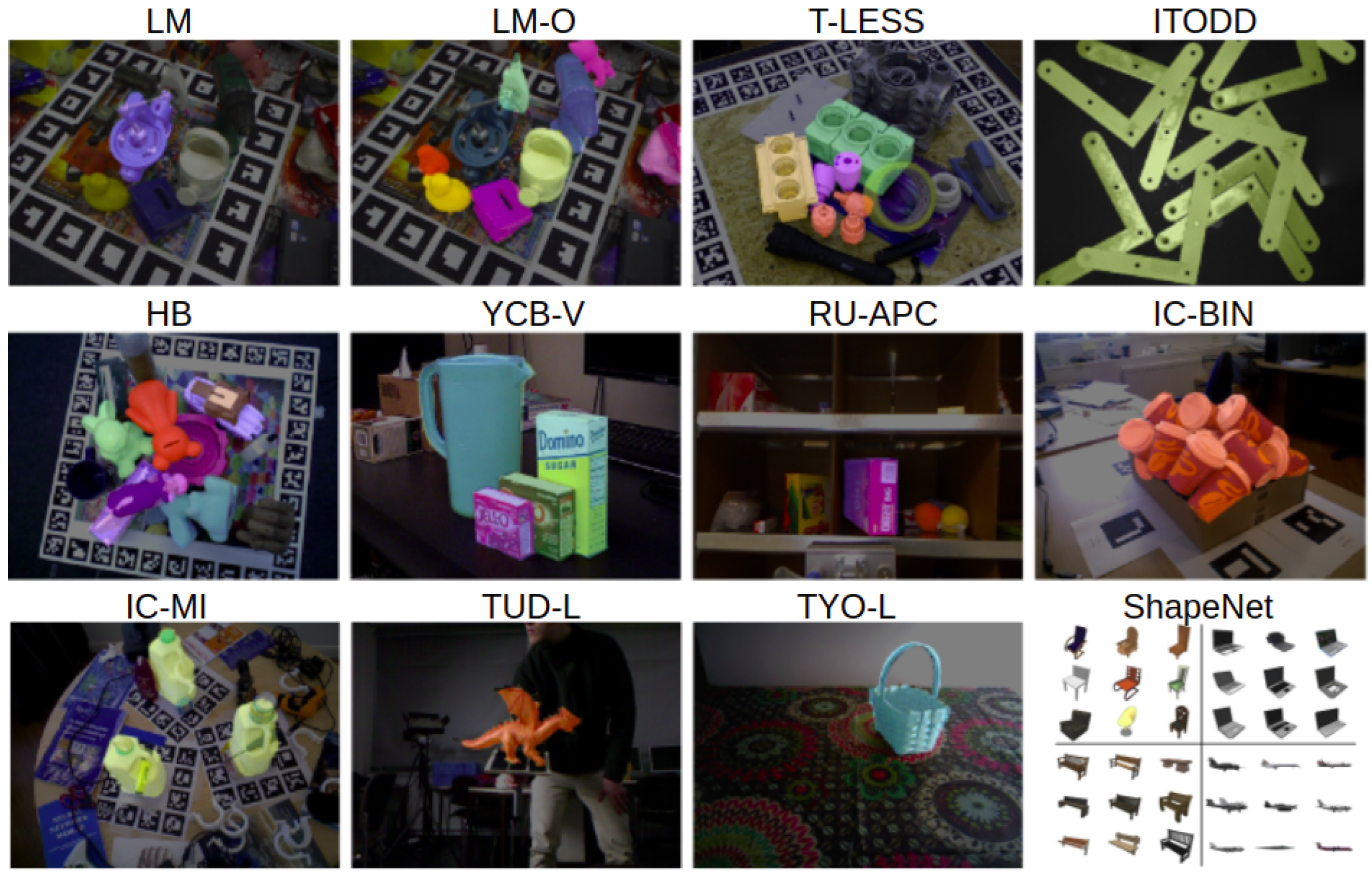
2. Related Work
3. Methodology
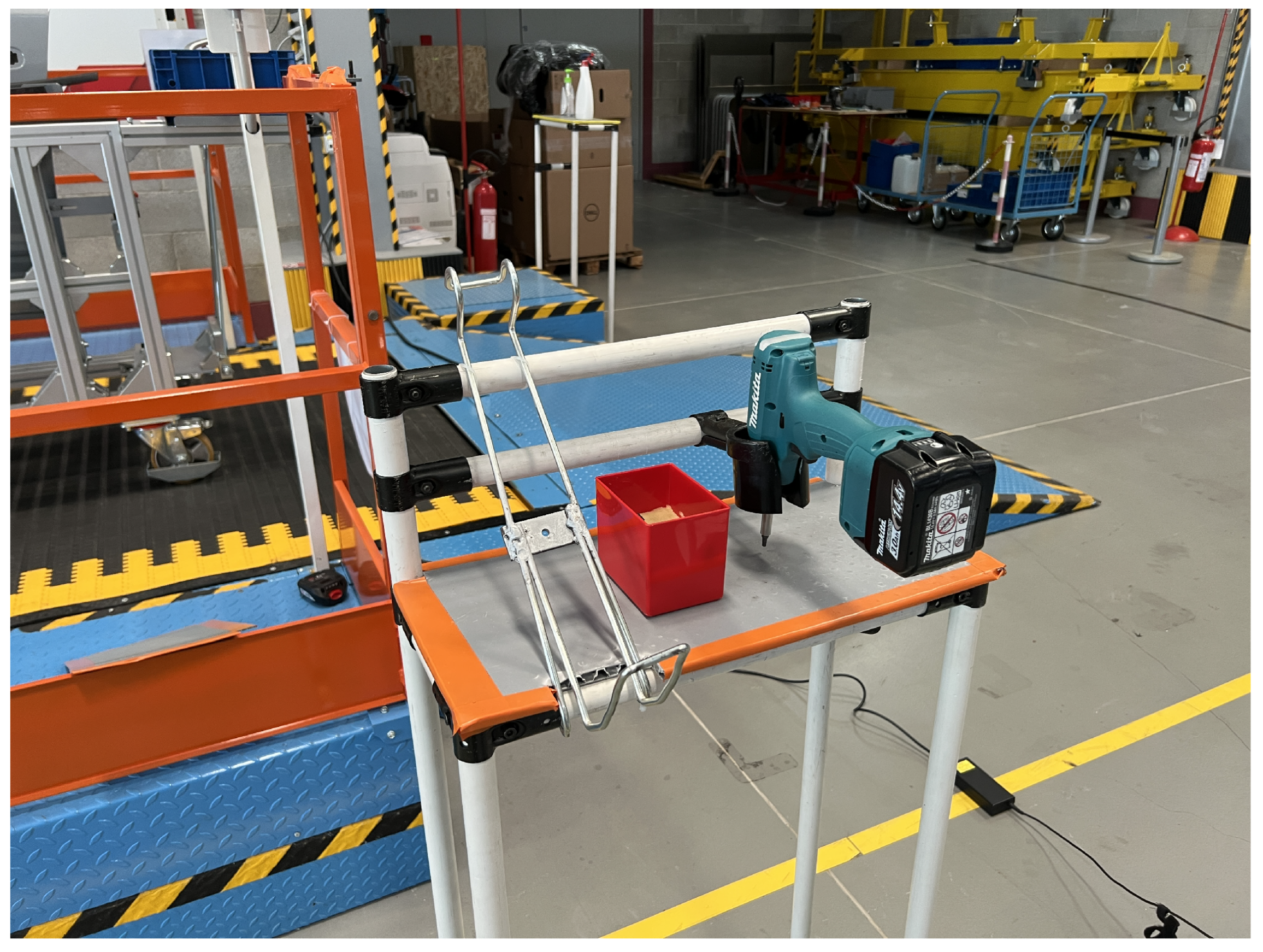
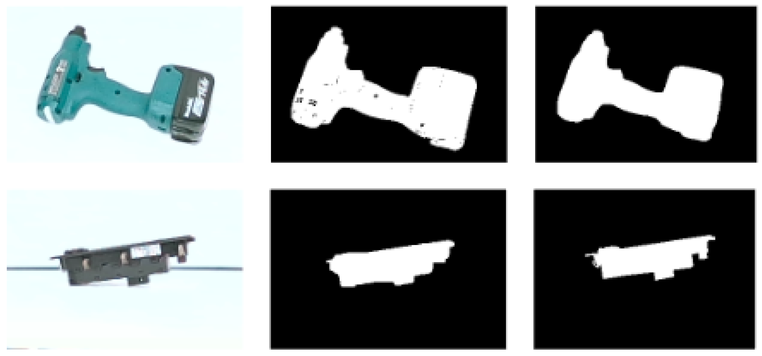
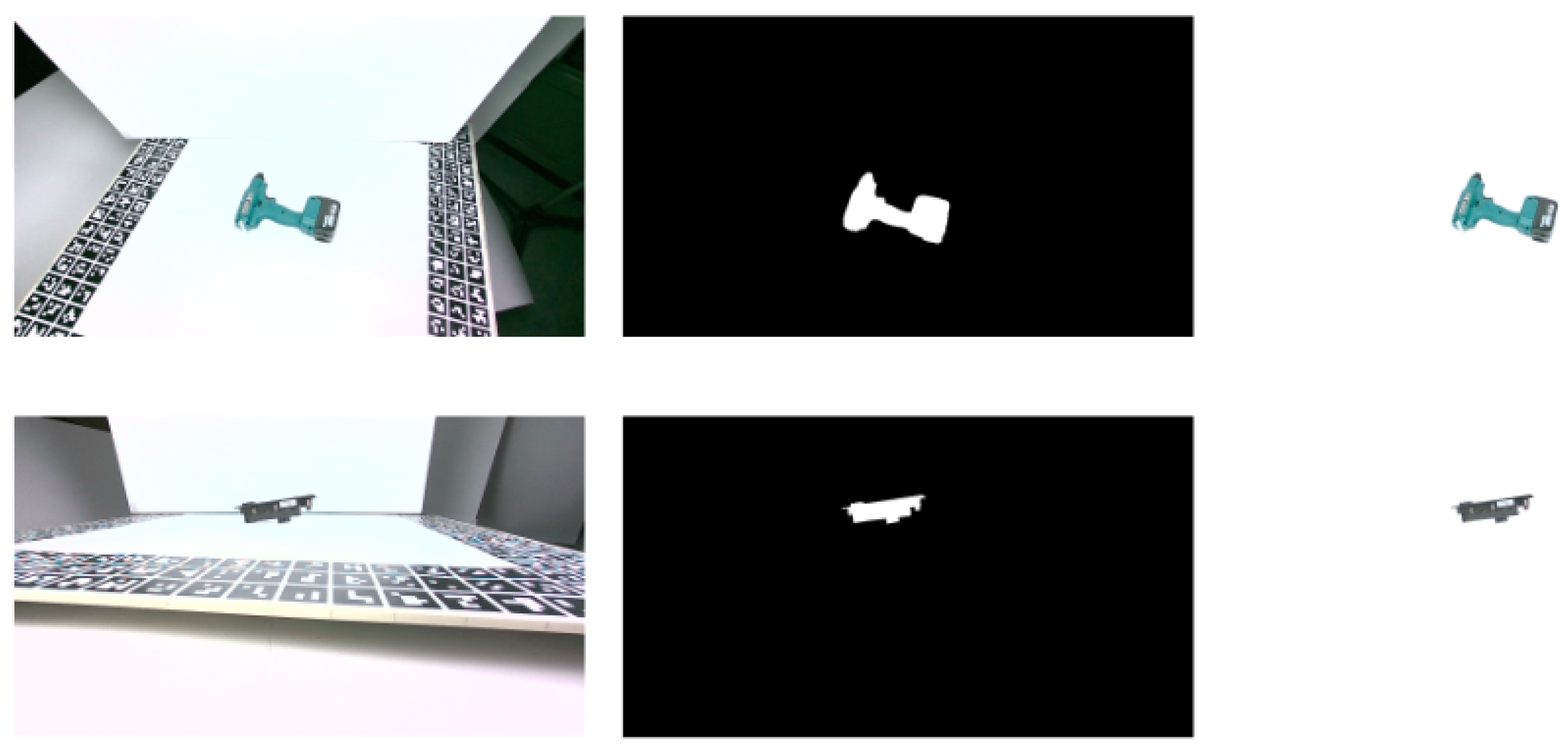
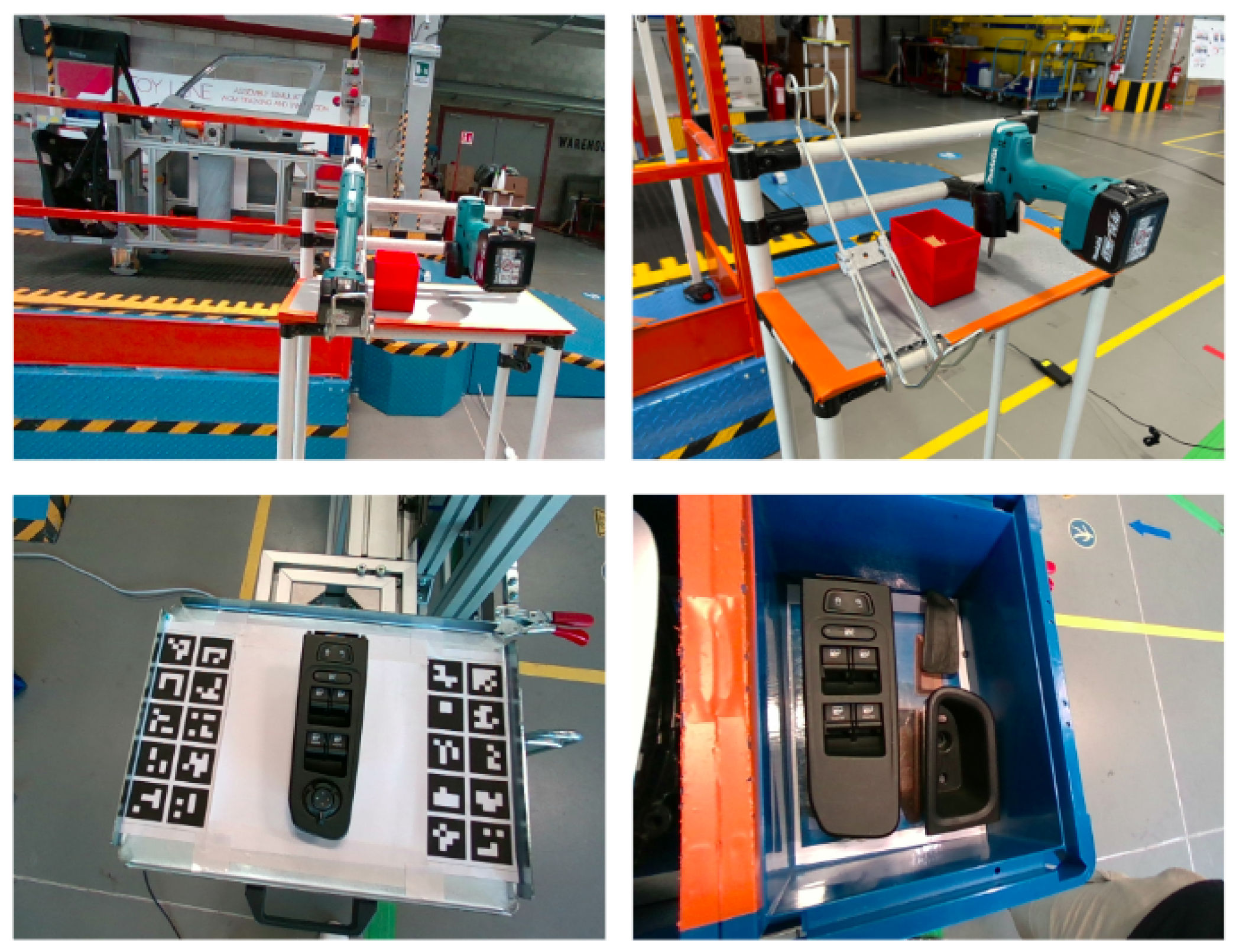
3.1. Challenging Objects and Environmental Conditions
3.2. Object Pose Estimation
3.3. Evaluation Metrics
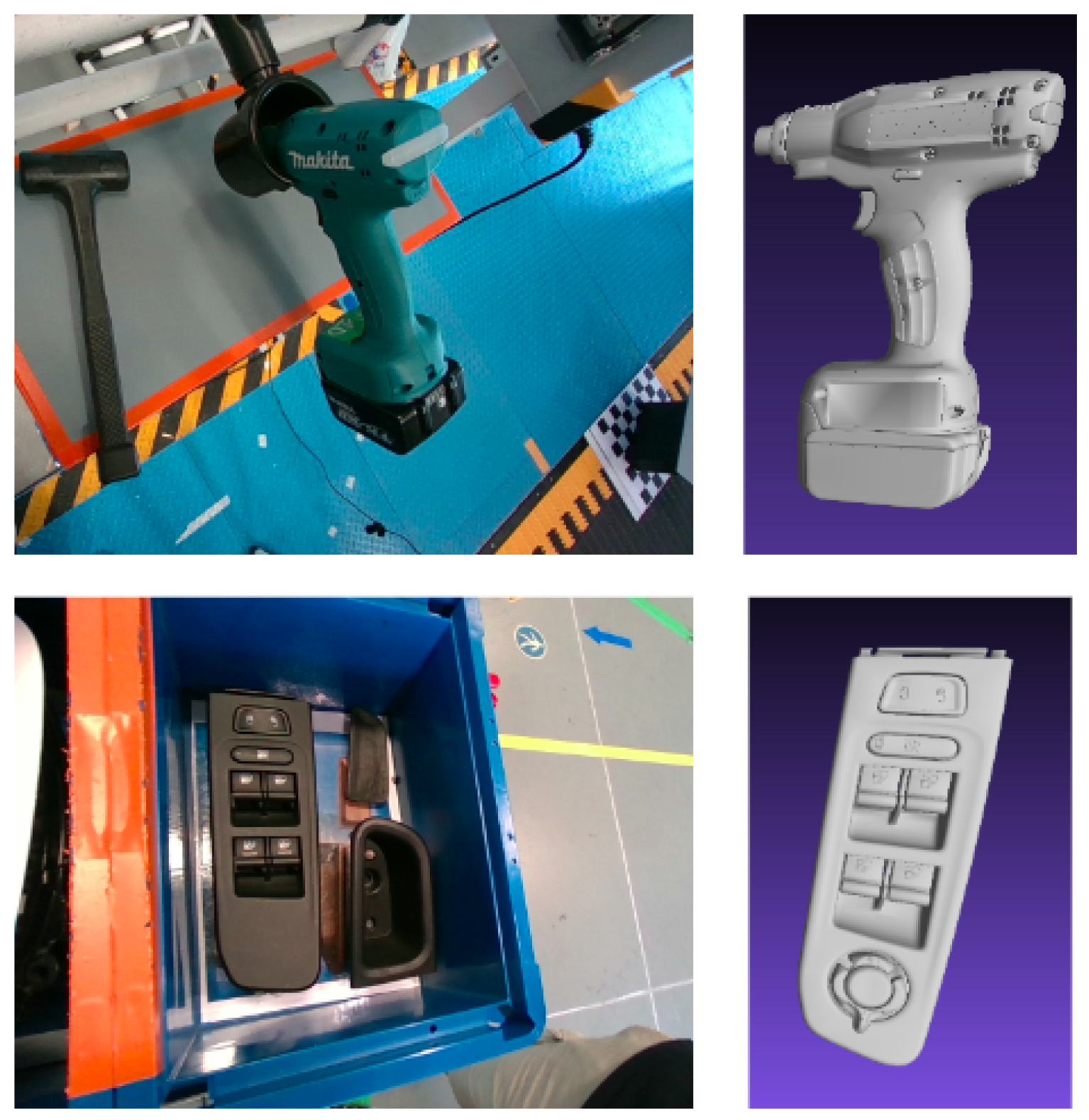
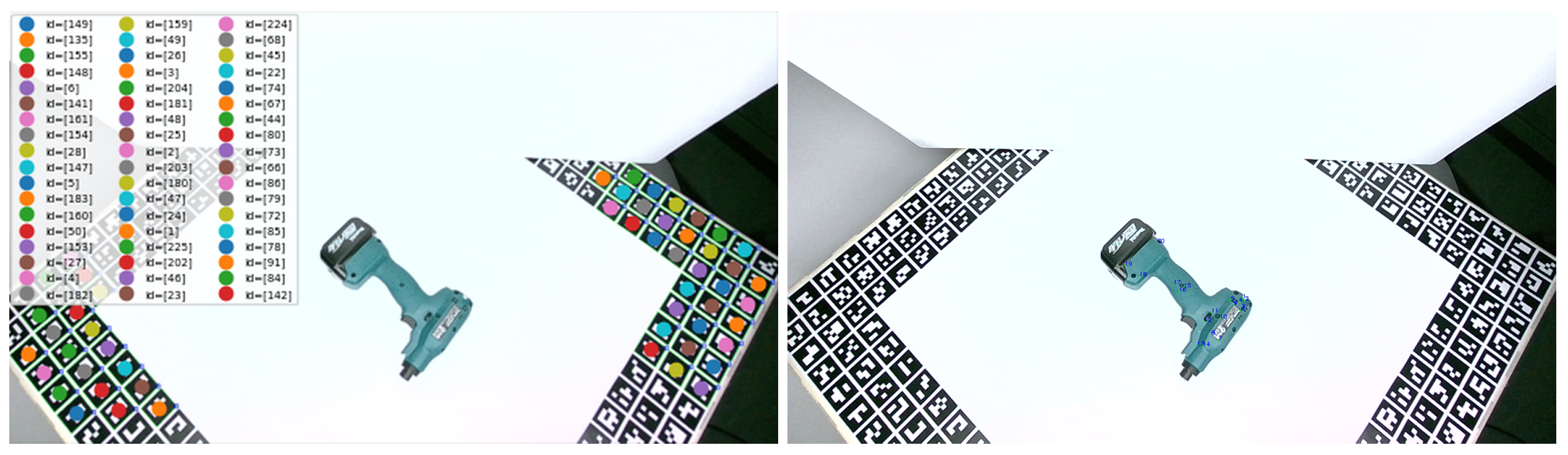
3.4. Object Models
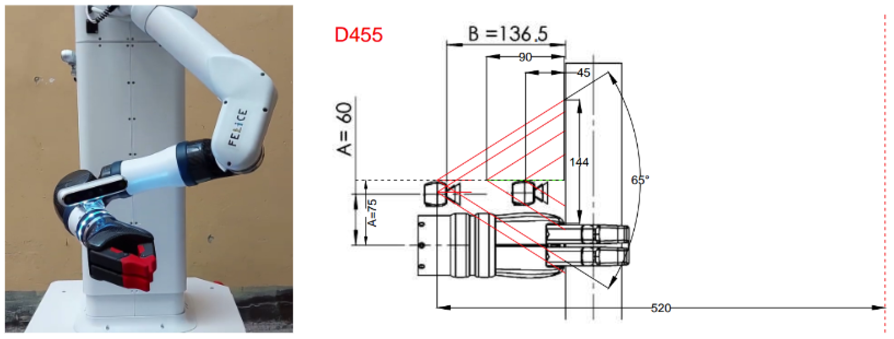
3.5. On-Robot Application/Integration
- ROS integration of RealSense2: The integration of the used RealSense camera was achieved through the wrapper provided by Intel. A ROS node was created to receive aligned images and camera calibration parameters from the RealSense camera, that would be further used as inputs for the object pose estimation.
- Detection and Localization node: The functionality of the object localization was integrated into ROS using a ROS package. This package contains a node that receives the input data from the RealSense camera and runs the object detection and localization as an on-demand ROS service, requested to localize an object, and the results are further communicated through a ROS message.
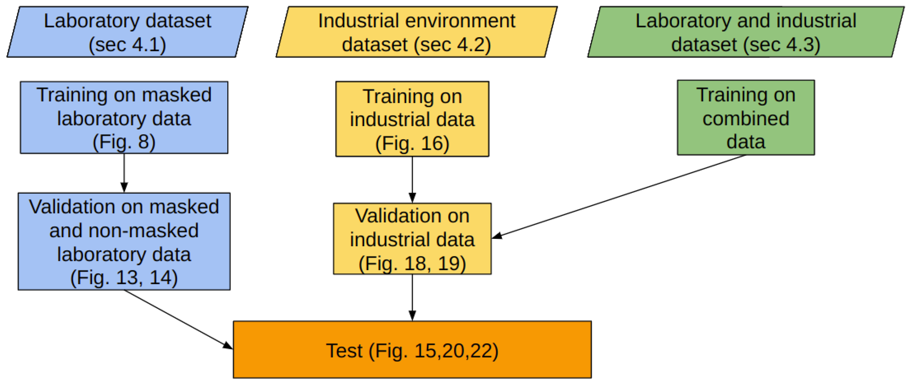
4. Experiments and Results
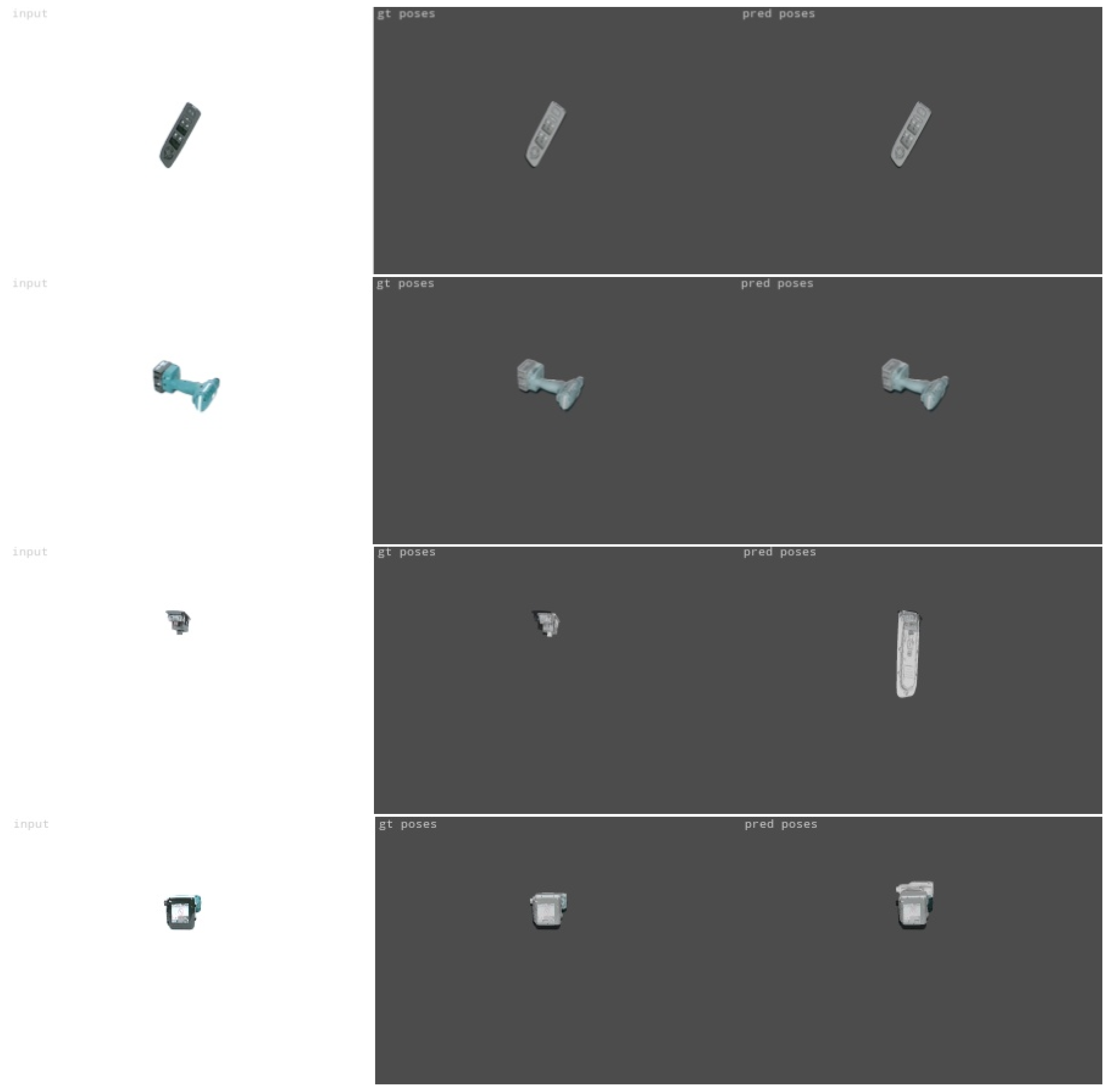
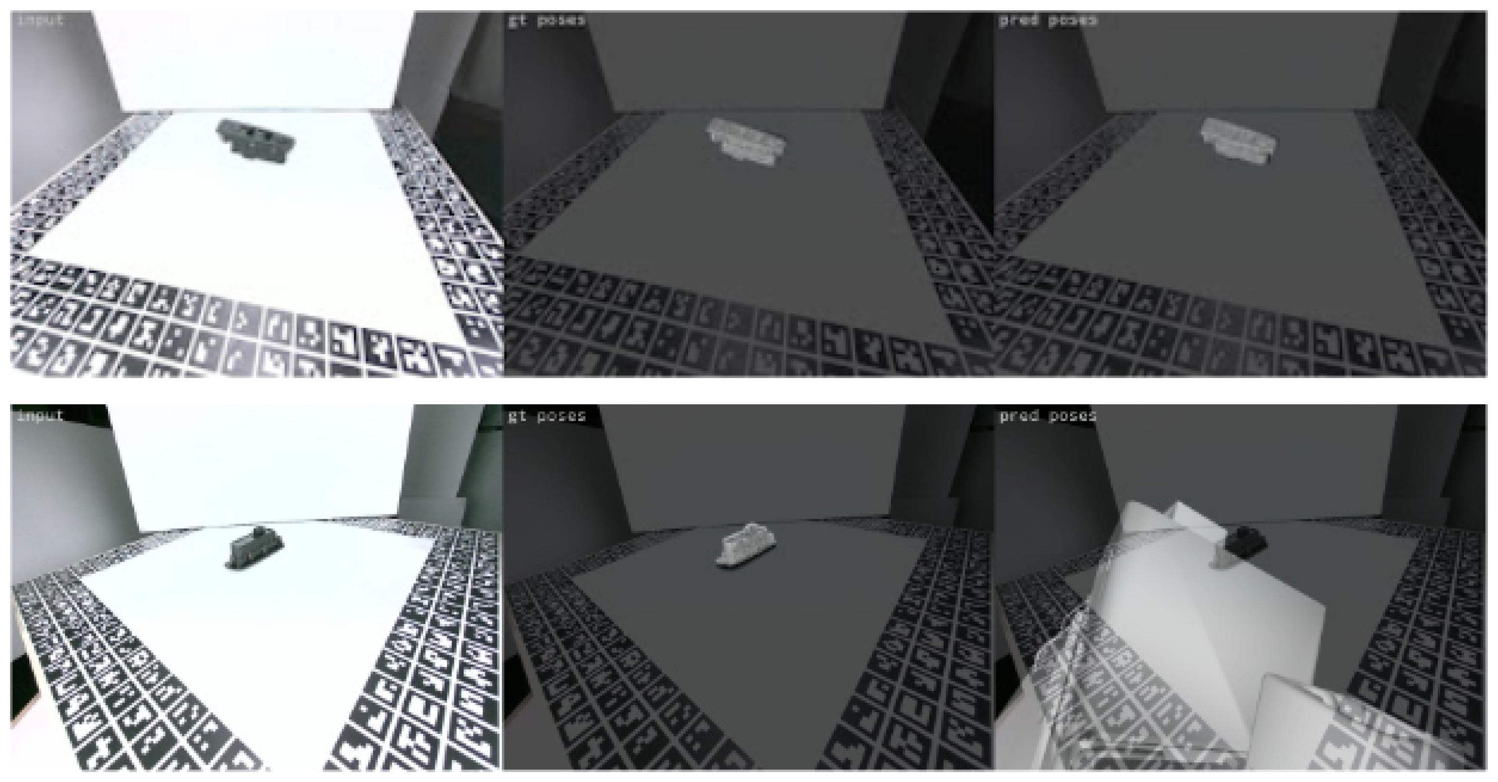
4.1. Model Trained on Laboratory Data
4.1.1. Datasets
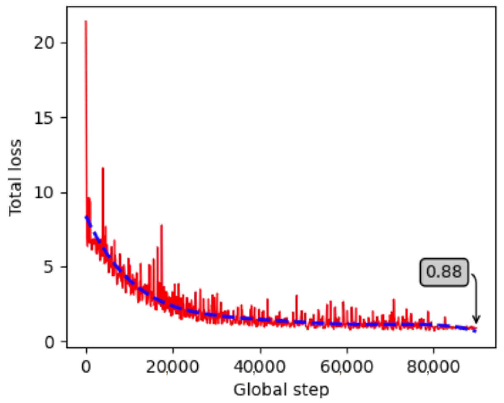
4.1.2. Training, Validation and Testing Results
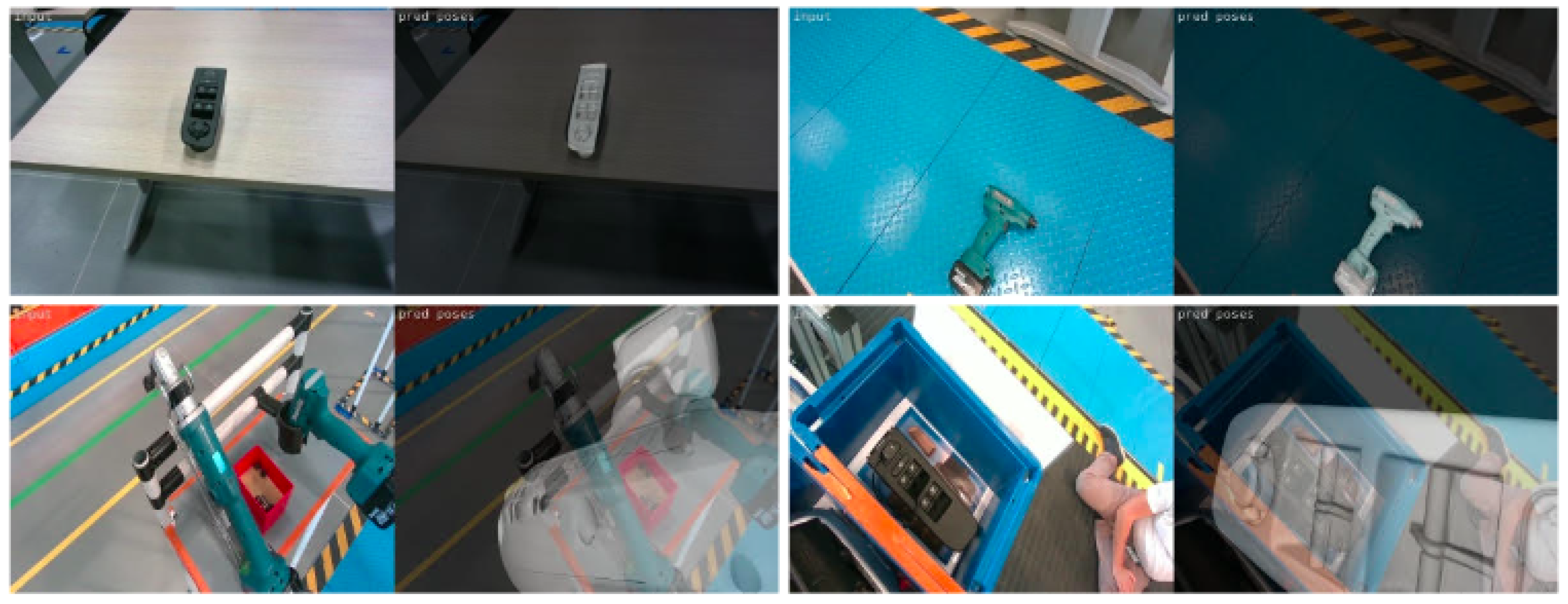
4.2. Model Trained on Real Industrial Environment Data
4.2.1. Datasets
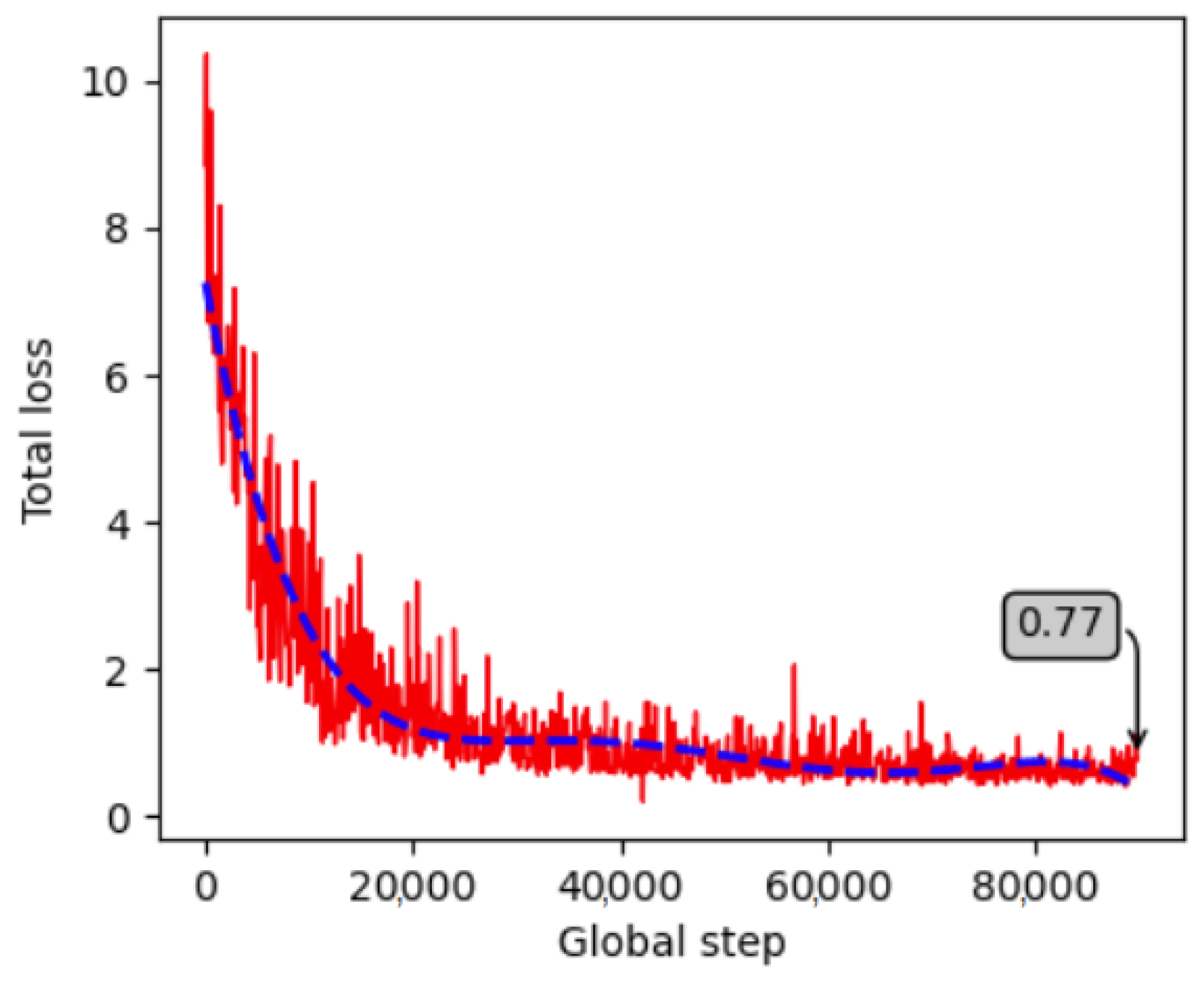
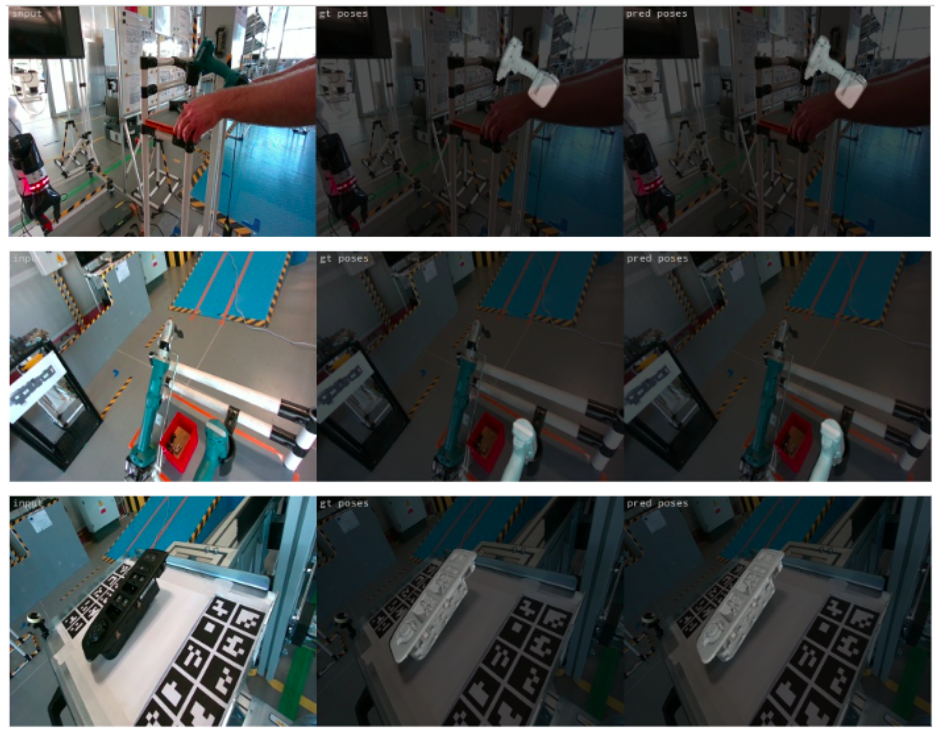
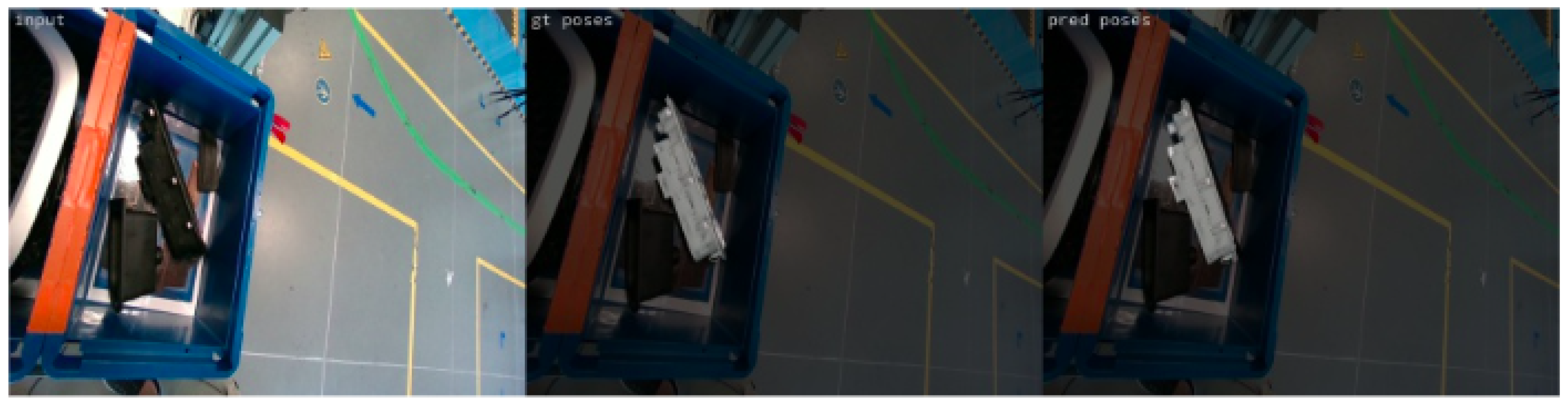
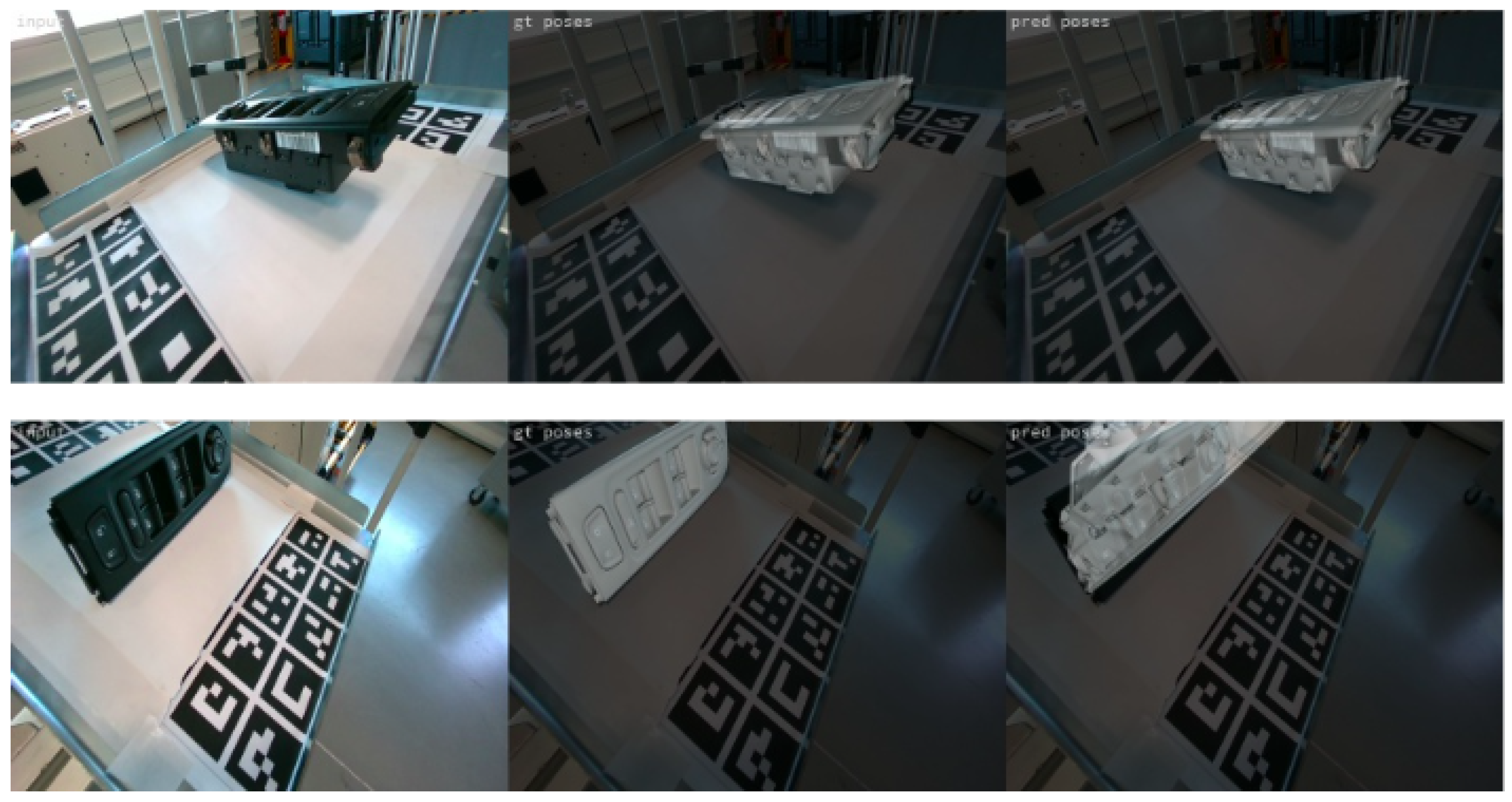
4.2.2. Training, Validation and Testing Results
4.3. Model Trained on Both the Laboratory and the Real Industrial Environment Data
4.3.1. Datasets
4.3.2. Training, Validation and Testing Results
5. Conclusions
Author Contributions
Funding
Institutional Review Board Statement
Informed Consent Statement
Data Availability Statement
Acknowledgments
Conflicts of Interest
References
- Hodaň, T.; Baráth, D.; Matas, J. EPOS: Estimating 6D Pose of Objects with Symmetries. In Proceedings of the IEEE Conference on Computer Vision and Pattern Recognition (CVPR), Virtual, 14–19 June 2020. [Google Scholar]
- Clement, F.; Shah, K.; Pancholi, D. A Review of methods for Textureless Object Recognition. arXiv 2019, arXiv:1910.14255. [Google Scholar]
- Du, G.; Wang, K.; Lian, S.; Zhao, K. Vision-based robotic grasping from object localization, object pose estimation to grasp estimation for parallel grippers: A review. Artif. Intell. Rev. 2021, 54, 1677–1734. [Google Scholar] [CrossRef]
- Kim, S.H.; Hwang, Y. A Survey on Deep learning-based Methods and Datasets for Monocular 3D Object Detection. Electronics 2021, 10, 517. [Google Scholar] [CrossRef]
- He, Z.; Feng, W.; Zhao, X.; Lv, Y. 6D Pose Estimation of Objects: Recent Technologies and Challenges. Appl. Sci. 2021, 11, 228. [Google Scholar] [CrossRef]
- Sahin, C.; Kim, T.K. Recovering 6D object pose: A review and multi-modal analysis. In Proceedings of the European Conference on Computer Vision (ECCV) Workshops, Munich, Germany, 8–14 September 2018. [Google Scholar]
- Rahman, M.M.; Tan, Y.; Xue, J.; Lu, K. Recent advances in 3D object detection in the era of deep neural networks: A survey. IEEE Trans. Image Process. 2019, 29, 2947–2962. [Google Scholar] [CrossRef] [PubMed]
- Wu, J.; Yin, D.; Chen, J.; Wu, Y.; Si, H.; Lin, K. A Survey on Monocular 3D Object Detection Algorithms Based on Deep Learning. J. Phys. Conf. Ser. 2020, 1518, 012049. [Google Scholar] [CrossRef]
- Shi, Y.; Huang, J.; Xu, X.; Zhang, Y.; Xu, K. StablePose: Learning 6D Object Poses from Geometrically Stable Patches. arXiv 2021, arXiv:2102.09334. [Google Scholar]
- Labbe, Y.; Carpentier, J.; Aubry, M.; Sivic, J. CosyPose: Consistent multi-view multi-object 6D pose estimation. In Proceedings of the European Conference on Computer Vision (ECCV), Glasgow, UK, 23–28 August 2020. [Google Scholar]
- Jiang, X.; Li, D.; Chen, H.; Zheng, Y.; Zhao, R.; Wu, L. Uni6D: A Unified CNN Framework without Projection Breakdown for 6D Pose Estimation. In Proceedings of the IEEE/CVF Conference on Computer Vision and Pattern Recognition, New Orleans, LA, USA, 18–22 June 2022; pp. 11174–11184. [Google Scholar]
- Various authors. Papers with Code—6D Pose Estimation Using RGB. 2021. Available online: https://paperswithcode.com/task/6d-pose-estimation (accessed on 30 December 2022).
- Hodaň, T.; Sundermeyer, M.; Drost, B.; Labbé, Y.; Brachmann, E.; Michel, F.; Rother, C.; Matas, J. BOP challenge 2020 on 6D object localization. In Proceedings of the European Conference on Computer Vision, Glasgow, UK, 23–28 August 2020; Springer: Berlin/Heidelberg, Germany, 2020; pp. 577–594. [Google Scholar]
- Park, K.; Patten, T.; Vincze, M. Pix2Pose: Pixel-wise coordinate regression of objects for 6D pose estimation. In Proceedings of the IEEE/CVF International Conference on Computer Vision, Seoul, Republic of Korea, 27 October–2 November 2019; pp. 7668–7677. [Google Scholar]
- Li, Y.; Wang, G.; Ji, X.; Xiang, Y.; Fox, D. DeepIM: Deep iterative matching for 6D pose estimation. In Proceedings of the European Conference on Computer Vision (ECCV), Munich, Germany, 8–14 September 2018; pp. 683–698. [Google Scholar]
- Tan, M.; Le, Q. EfficientNet: Rethinking model scaling for convolutional neural networks. In Proceedings of the International Conference on Machine Learning, PMLR, Long Beach, CA, USA, 9–15 June 2019; pp. 6105–6114. [Google Scholar]
- Dosovitskiy, A.; Fischer, P.; Ilg, E.; Hausser, P.; Hazirbas, C.; Golkov, V.; Van Der Smagt, P.; Cremers, D.; Brox, T. FlowNet: Learning optical flow with convolutional networks. In Proceedings of the IEEE International Conference on Computer Vision, Santiago, Chile, 7–13 December 2015; pp. 2758–2766. [Google Scholar]
- Lepetit, V.; Moreno-Noguer, F.; Fua, P. EPnP: An accurate O(n) solution to the PnP problem. Int. J. Comput. Vis. 2009, 81, 155. [Google Scholar] [CrossRef] [Green Version]
- Fischler, M.A.; Bolles, R.C. Random sample consensus: A paradigm for model fitting with applications to image analysis and automated cartography. Commun. ACM 1981, 24, 381–395. [Google Scholar] [CrossRef]
- Jin, M.; Li, J.; Zhang, L. DOPE++: 6D pose estimation algorithm for weakly textured objects based on deep neural networks. PLoS ONE 2022, 17, e0269175. [Google Scholar] [CrossRef] [PubMed]
- He, Y.; Sun, W.; Huang, H.; Liu, J.; Fan, H.; Sun, J. PVN3D: A Deep Point-wise 3D Keypoints Voting Network for 6DoF Pose Estimation. In Proceedings of the IEEE/CVF Conference on Computer Vision and Pattern Recognition, Seattle, WA, USA, 13–19 June 2020; pp. 11632–11641. [Google Scholar]
- He, Y.; Huang, H.; Fan, H.; Chen, Q.; Sun, J. Ffb6d: A full flow bidirectional fusion network for 6D pose estimation. In Proceedings of the IEEE/CVF Conference on Computer Vision and Pattern Recognition, Nashville, TN, USA, 20–25 June 2021; pp. 3003–3013. [Google Scholar]
- He, Y.; Wang, Y.; Fan, H.; Sun, J.; Chen, Q. FS6D: Few-Shot 6D Pose Estimation of Novel Objects. In Proceedings of the IEEE/CVF Conference on Computer Vision and Pattern Recognition, New Orleans, LA, USA, 18–24 June 2022; pp. 6814–6824. [Google Scholar]
- Cao, T.; Luo, F.; Fu, Y.; Zhang, W.; Zheng, S.; Xiao, C. DGECN: A Depth-Guided Edge Convolutional Network for End-to-End 6D Pose Estimation. In Proceedings of the IEEE/CVF Conference on Computer Vision and Pattern Recognition, New Orleans, LA, USA, 18–24 June 2022; pp. 3783–3792. [Google Scholar]
- He, Z.; Zhang, L. Multi-adversarial faster-RCNN for unrestricted object detection. In Proceedings of the IEEE/CVF International Conference on Computer Vision, Seoul, Republic of Korea, 27–28 October 2019; pp. 6668–6677. [Google Scholar]
- Li, F.; Yu, H.; Shugurov, I.; Busam, B.; Yang, S.; Ilic, S. NeRF-Pose: A First-Reconstruct-Then-Regress Approach for Weakly-supervised 6D Object Pose Estimation. arXiv 2022, arXiv:2203.04802. [Google Scholar]
- Hinterstoisser, S.; Lepetit, V.; Ilic, S.; Holzer, S.; Bradski, G.; Konolige, K.; Navab, N. Model based training, detection and pose estimation of texture-less 3D objects in heavily cluttered scenes. In Proceedings of the Asian Conference on Computer Vision, Daejeon, Republic of Korea, 5–9 November 2012; Springer: Berlin/Heidelberg, Germany, 2012; pp. 548–562. [Google Scholar]
- Brachmann, E.; Krull, A.; Michel, F.; Gumhold, S.; Shotton, J.; Rother, C. Learning 6D object pose estimation using 3D object coordinates. In Proceedings of the European Conference on Computer Vision, Zurich, Switzerland, 6–12 September 2014; Springer: Berlin/Heidelberg, Germany, 2014; pp. 536–551. [Google Scholar]
- Kaskman, R.; Zakharov, S.; Shugurov, I.; Ilic, S. Homebreweddb: RGB-D dataset for 6D pose estimation of 3D objects. In Proceedings of the IEEE/CVF International Conference on Computer Vision Workshops, Seoul, Republic of Korea, 27 October–2 November 2019. [Google Scholar]
- Rennie, C.; Shome, R.; Bekris, K.E.; De Souza, A.F. A dataset for improved RGBD-based object detection and pose estimation for warehouse pick-and-place. IEEE Robot. Autom. Lett. 2016, 1, 1179–1185. [Google Scholar] [CrossRef] [Green Version]
- Tejani, A.; Tang, D.; Kouskouridas, R.; Kim, T.K. Latent-class Hough forests for 3D object detection and pose estimation. In Proceedings of the European Conference on Computer Vision, Zurich, Switzerland, 6–12 September 2014; Springer: Berlin/Heidelberg, Germany, 2014; pp. 462–477. [Google Scholar]
- Xiang, Y.; Schmidt, T.; Narayanan, V.; Fox, D. PoseCNN: A convolutional neural network for 6D object pose estimation in cluttered scenes. arXiv 2017, arXiv:1711.00199. [Google Scholar]
- Hodan, T.; Haluza, P.; Obdržálek, Š.; Matas, J.; Lourakis, M.; Zabulis, X. T-LESS: An RGB-D dataset for 6D pose estimation of texture-less objects. In Proceedings of the 2017 IEEE Winter Conference on Applications of Computer Vision (WACV), Santa Rosa, CA, USA, 24–31 March 2017; IEEE: Piscataway, NJ, USA, 2017; pp. 880–888. [Google Scholar]
- Drost, B.; Ulrich, M.; Bergmann, P.; Hartinger, P.; Steger, C. Introducing MVTec ITODD—A dataset for 3D object recognition in industry. In Proceedings of the IEEE International Conference on Computer Vision Workshops, Venice, Italy, 22–29 October 2017; pp. 2200–2208. [Google Scholar]
- Doumanoglou, A.; Kouskouridas, R.; Malassiotis, S.; Kim, T.K. Recovering 6D object pose and predicting next-best-view in the crowd. In Proceedings of the IEEE Conference on Computer Vision and Pattern Recognition, Las Vegas, NV, USA, 26 June–1 July 2016; pp. 3583–3592. [Google Scholar]
- Chang, A.X.; Funkhouser, T.; Guibas, L.; Hanrahan, P.; Huang, Q.; Li, Z.; Savarese, S.; Savva, M.; Song, S.; Su, H.; et al. Shapenet: An information-rich 3D model repository. arXiv 2015, arXiv:1512.03012. [Google Scholar]
- Byambaa, M.; Koutaki, G.; Choimaa, L. 6D Pose Estimation of Transparent Objects Using Synthetic Data. In Proceedings of the International Workshop on Frontiers of Computer Vision, Virtual, 21–22 February 2022; Springer: Berlin/Heidelberg, Germany, 2022; pp. 3–17. [Google Scholar]
- Hodan, T.; Michel, F.; Brachmann, E.; Kehl, W.; GlentBuch, A.; Kraft, D.; Drost, B.; Vidal, J.; Ihrke, S.; Zabulis, X.; et al. BOP: Benchmark for 6D object pose estimation. In Proceedings of the European Conference on Computer Vision (ECCV), Munich, Germany, 8–14 September 2018; pp. 19–34. [Google Scholar]
- Chen, L.C.; Zhu, Y.; Papandreou, G.; Schroff, F.; Adam, H. encoder–decoder with atrous separable convolution for semantic image segmentation. In Proceedings of the European Conference on Computer Vision (ECCV), Munich, Germany, 8–14 September 2018; pp. 801–818. [Google Scholar]
- Huber, P.J. Robust estimation of a location parameter. In Breakthroughs in Statistics; Springer: Berlin/Heidelberg, Germany, 1992; pp. 492–518. [Google Scholar]
- Barath, D.; Matas, J. Progressive-x: Efficient, anytime, multi-model fitting algorithm. In Proceedings of the IEEE/CVF international Conference on Computer Vision, Seoul, Republic of Korea, 27–28 October 2019; pp. 3780–3788. [Google Scholar]
- Barath, D.; Matas, J. Graph-cut RANSAC. In Proceedings of the IEEE Conference on Computer Vision and Pattern Recognition, Salt Lake City, UT, USA, 18–23 June 2018; pp. 6733–6741. [Google Scholar]
- Kneip, L.; Scaramuzza, D.; Siegwart, R. A novel parametrization of the perspective-three-point problem for a direct computation of absolute camera position and orientation. In Proceedings of the CVPR 2011, Springs, CO, USA, 20–25 June 2011; IEEE: Piscataway, NJ, USA, 2011; pp. 2969–2976. [Google Scholar]
- Moré, J.J. The Levenberg-Marquardt algorithm: Implementation and theory. In Numerical Analysis; Springer: Berlin/Heidelberg, Germany, 1978; pp. 105–116. [Google Scholar]
- Hodaň, T.; Matas, J.; Obdržálek, Š. On evaluation of 6D object pose estimation. In Proceedings of the European Conference on Computer Vision, Amsterdam, The Netherlands, 11–14 October 2016; Springer: Berlin/Heidelberg, Germany, 2016; pp. 606–619. [Google Scholar]
- Ronneberger, O.; Fischer, P.; Brox, T. U-net: Convolutional networks for biomedical image segmentation. In Proceedings of the International Conference on Medical Image Computing and Computer-Assisted Intervention, Munich, Germany, 5–9 October 2015; Springer: Berlin/Heidelberg, Germany, 2015; pp. 234–241. [Google Scholar]
- Cignoni, P.; Callieri, M.; Corsini, M.; Dellepiane, M.; Ganovelli, F.; Ranzuglia, G. Meshlab: An open-source mesh processing tool. In Proceedings of the Eurographics Italian Chapter Conference, Salerno, Italy, 2–4 July 2008; Volume 2008, pp. 129–136. [Google Scholar]
- Intel RealSense Depth Camera D455. Available online: https://www.intelrealsense.com/depth-camera-d455/ (accessed on 21 July 2022).
- Garrido-Jurado, S.; Muñoz Salinas, R.; Madrid-Cuevas, F.; Marín-Jiménez, M. Automatic Generation and Detection of Highly Reliable Fiducial Markers under Occlusion. Pattern Recognit. 2014, 47, 2280–2292. [Google Scholar] [CrossRef]
- Long, J.; Shelhamer, E.; Darrell, T. Fully convolutional networks for semantic segmentation. In Proceedings of the IEEE Conference on Computer Vision and Pattern Recognition, Boston, MA, USA, 7–12 June 2015; pp. 3431–3440. [Google Scholar]
- Chen, L.C.; Papandreou, G.; Schroff, F.; Adam, H. Rethinking atrous convolution for semantic image segmentation. arXiv 2017, arXiv:1706.05587. [Google Scholar]
- Badrinarayanan, V.; Kendall, A.; Cipolla, R. Segnet: A deep convolutional encoder–decoder architecture for image segmentation. IEEE Trans. Pattern Anal. Mach. Intell. 2017, 39, 2481–2495. [Google Scholar] [CrossRef] [PubMed]
- Lourakis, M. Posest: A C/C++ Library for Robust 6DoF Pose Estimation from 3D-2D Correspondences. Available online: https://users.ics.forth.gr/~lourakis/posest/ (accessed on 21 July 2022).
- Lourakis, M.; Zabulis, X. Model-based pose estimation for rigid objects. In Proceedings of the International Conference on Computer Vision Systems, St. Petersburg, Russia, 16–18 July 2013; Springer: Berlin/Heidelberg, Germany, 2013; pp. 83–92. [Google Scholar]
- Chollet, F. Xception: Deep learning with depthwise separable convolutions. In Proceedings of the IEEE Conference on Computer Vision and Pattern Recognition, Honolulu, HI, USA, 21–26 July 2017; pp. 1251–1258. [Google Scholar]
- Deng, J.; Dong, W.; Socher, R.; Li, L.J.; Li, K.; Fei-Fei, L. Imagenet: A large-scale hierarchical image database. In Proceedings of the 2009 IEEE Conference on Computer Vision and Pattern Recognition, Miami, FL, USA, 20–25 June 2009; IEEE: Piscataway, NJ, USA, 2009; pp. 248–255. [Google Scholar]
- Lin, T.Y.; Maire, M.; Belongie, S.; Hays, J.; Perona, P.; Ramanan, D.; Dollár, P.; Zitnick, C.L. Microsoft COCO: Common objects in context. In Proceedings of the European Conference on Computer Vision, Zurich, Switzerland, 6–12 September 2014; Springer: Berlin/Heidelberg, Germany, 2014; pp. 740–755. [Google Scholar]
- Hinterstoisser, S.; Lepetit, V.; Wohlhart, P.; Konolige, K. On pre-trained image features and synthetic images for deep learning. In Proceedings of the European Conference on Computer Vision (ECCV) Workshops, Munich, Germany, 8–14 September 2018. [Google Scholar]
- Blume, F. 6DPAT. Available online: https://github.com/florianblume/6d-pat (accessed on 30 December 2022).


| Recall (%) | MSSD | MSPD | ADD | VSD | Average (MSSD, MSPD, VSD) |
|---|---|---|---|---|---|
| Masked Images | 98.3 | 99.1 | 97.1 | 96.0 | 97.8 |
| NON Masked Images | 50.3 | 54.0 | 44.4 | 48.3 | 50.9 |
| Recall (%) | MSSD | MSPD | ADD | VSD | Average (MSSD, MSPD, VSD) |
|---|---|---|---|---|---|
| Real Environment Images | 94.5 | 95.2 | 96.7 | 94.3 | 94.7 |
| Recall (%) | MSSD | MSPD | ADD | VSD | Average (MSSD, MSPD, VSD) |
|---|---|---|---|---|---|
| Laboratory and Real Environment Images | 94.6 | 95.0 | 96.0 | 94.6 | 94.7 |
Disclaimer/Publisher’s Note: The statements, opinions and data contained in all publications are solely those of the individual author(s) and contributor(s) and not of MDPI and/or the editor(s). MDPI and/or the editor(s) disclaim responsibility for any injury to people or property resulting from any ideas, methods, instructions or products referred to in the content. |
© 2023 by the authors. Licensee MDPI, Basel, Switzerland. This article is an open access article distributed under the terms and conditions of the Creative Commons Attribution (CC BY) license (https://creativecommons.org/licenses/by/4.0/).
Share and Cite
Papadaki, A.; Pateraki, M. 6D Object Localization in Car-Assembly Industrial Environment. J. Imaging 2023, 9, 72. https://doi.org/10.3390/jimaging9030072
Papadaki A, Pateraki M. 6D Object Localization in Car-Assembly Industrial Environment. Journal of Imaging. 2023; 9(3):72. https://doi.org/10.3390/jimaging9030072
Chicago/Turabian StylePapadaki, Alexandra, and Maria Pateraki. 2023. "6D Object Localization in Car-Assembly Industrial Environment" Journal of Imaging 9, no. 3: 72. https://doi.org/10.3390/jimaging9030072