An Accurate Activate Screw Detection Method for Automatic Electric Vehicle Battery Disassembly

Abstract

With the increasing popularity of electric vehicles, the number of end-of-life (EOF) electric vehicle batteries (EVBs) is also increasing day by day. Efficient dismantling and recycling of EVBs are essential to ensure environmental protection. There are many types of EVBs with complex structures, and the current automatic dismantling line is immature and lacks corresponding dismantling equipment. This makes it difficult for some small parts to be disassembled precisely. Screws are used extensively in batteries to fix or connect modules in EVBs. However, due to the small size of screws and differences in installation angles, screw detection is a very challenging task and a significant obstacle to automatic EVBs disassembly. This research proposes a systematic method to complete screw detection called “Active Screw Detection”. The experimental results show that with the YOLOX-s model, the improved YOLOX model achieves $95.92\%$ and $92.14\%$ accuracy for both $mA{P}_{50}$ and $mA{P}_{75}$ positioning after autonomous adjustment of the robotic arm attitude. Compared to the method without autonomous adjustment of the robotic arm, $mA{P}_{50}$ and $mA{P}_{75}$ improved by $62.81\%$ and $57.67\%$, respectively. In addition, the improved YOLOX model improves $mA{P}_{50}$ and $mA{P}_{75}$ by $0.19\%$ and $3.59\%$, respectively, compared to the original YOLOX model.

1. Introduction

With the rapid growth of EVBs [1], the EVB industry has developed rapidly in recent years [2]. EOF batteries contain a large amount of renewable resources and have gathered considerable attention [3]. The recycling [4] and dismantling [5] of EOF EVBs have become a hot topic. EVBs, a class of electronic waste (E-Waste), contain heavy metals and other harmful substances, which can contaminate the soil and water, thus damaging the environment and affecting human health [6,7,8,9]. The safety of the battery itself also needs to be considered [10]. At the same time, in recycling EOF EVBs, the control circuit, thermal management system, and other standardized parts connected to the battery can be recycled intact [11]. The electrode materials of battery modules contain valuable elements, such as Li, Co, Ni, and Mn [12]. The current mainstream recovery method uses wet metallurgy to separate these elements and make various pure oxides or carbonates [13]. Therefore, in terms of environmental protection and circular economy, recycling EOF electric vehicle batteries is necessary. Due to the wide variety of EOF EVBs and complex structures, the task of recycling and disassembling EVBs is currently mainly manual [14,15]. This is inefficient and exposes workers to dangerous working conditions [16], making it difficult to guarantee the safety of dismantled power batteries [17]. Compared to the manual disassembly of the screws using human hands, an integrated robotic arm disassembly system may save a lot of costs and avoid some safety accidents. Most of the current research on intelligent dismantling of EVBs has focused on the recycling of individual batteries, with few studies mentioning the process of dismantling and recycling parts in the form of bags/stacks. This is because of the problems of non-uniform standardization, different battery pack sizes, and different embedded battery specifications in the intelligent disassembly task [18]. So there is an urgent need to automate intelligent disassembly. Screws, the most numerous fasteners in electric vehicle battery cells, have been a challenge to locate and classify in intelligent disassembly tasks accurately. Unlike automated production, the location of screws on electric vehicle battery cells is uncertain, and the screws must be identified and positioned on site. The lack of identification accuracy restricts the use and popularity of automated disassembly assembly lines. So it is necessary to design an algorithm for the accurate location and classification of screws.

The screw detection task aims to detect the screws in the sensory field while obtaining information about the category of the screw and the accurate position for the subsequent disassembly task. In recent years, artificial intelligence technology has been developing rapidly in the field of object detection [19,20,21,22,23], and it only needs some annotated images for training the model to achieve high target localization accuracy [6,24,25,26]. However, the result of the direct application of these methods of screw detection is not as good as expected. For example: using the global camera to obtain RGB images and complete the screw detection task will result in many false and missed detections. First of all, the screws are installed at very different angles due to the complex structure of the battery pack. Moreover, the features of screws significantly change when observing them from different angles. Even worse, if the image capture position is inappropriate, some screws will be occluded and cannot be detected. So it is difficult to find a suitable global location, capture one image, and accurately identify all the screws in the battery pack. Few researchers have focused on this issue. On the other hand, the screw itself is a small object compared to the other parts in an EVB. The pixel area of small objects is small, and feature information is easily lost in common feature extraction operations [27,28,29]. This increases the difficulty of the screw detection task.

Most of the mechanically related tasks rely on visual information [30]. The role of vision sensors is similar to that of human eyes and is the main source of external information for robots. In tasks related to screw detection and localization based on visual information, most researchers have envisioned experiments in an ideal situation, paying little attention to the problem of increased difficulty in screw detection due to changes in the field of perception of the visual sensor during continuous disassembly. Throughout the process of screw detection, Yildiz, E. et al. [24] assumed that the camera had a vertical surface to the surface of the electronic device to be inspected, with the height set to 60 cm. This scenario is too idealistic and difficult to implement in real production because some screws are located in a plane that is not parallel to the horizontal plane or on the side of the battery pack. It is obvious that real production lines would prefer to develop a coherent screw positioning method that can be actively adjusted.

There are currently two main approaches to screw detection tasks based on visual information. One is based on a pre-programmed robot approach, where a predefined scan of an electric vehicle battery cell is performed to obtain a point cloud model of the pack. Then, operations such as feature matching are performed to obtain information on the position and size of the screws. L. Jurjević et al. [31] used the Two Xiaomi Yi camera to obtain a 3D point cloud of the object to construct a 3D model, but the model was not sufficiently detailed. Adjigble, M. et al. [32] obtained a point cloud of the object to be disassembled by scanning, calculated the zero moment displacement features on the point cloud, and extracting the same features on the point cloud of the fixture model, which were then used together to calculate the local shape between the object and the gripper similarity metric. The main idea is to find the point that maximizes the contact surface and to use only the area of the object that matches the surface curvature of the gripper fingers for gripping. Finally, a feasibility analysis was performed to select the subset of point pairs that returned from previous actions and were kinematically feasible for the gripper. Li, R. et al. [33] used a vision system to extract the approximate position and centre line of the screw in the part from an applicable CAD model to locate the screw. This type of method is currently mostly used on industrial production lines. However, this approach does not adapt to the disassembly strategy to the actual condition of the battery pack. The researchers mentioned that the method can be used only under ideal conditions. In practice, the screws themselves may fail (screw stuck, screw head damaged, etc.), which can affect the effectiveness of the method. In addition, the appearance of damaged cells or new structures of cells can affect the accuracy of the disassembly task. Another approach is to use machine learning methods to detect and locate screws based on 2D images captured by visual sensing. Gil, P. et al. [34] used the Canny operator to extract contours from images with screws and then used feature matching to classify and locate components. Cha, Y. J. et al. [35] performed Circle Hough Transform (CHT) after cropping the images to locate the circles on screw heads and washers in binarized images. Park, J. H. et al. [36] used the Canny operator to detect edges in images and then used Hough Transform (HT) and CHT to find lines and circle lines in images, respectively, to locate screws. The Canny operator was used to detect the edges in the image, and then HT and CHT were used to find the lines as well as the circle lines in the image to localize the screw, respectively. Pan, X. et al. [37] proposed that the HT algorithm using Canny, Prewitt, and Log methods could not accurately detect the lines and circles in complex images. The reason is that the HT algorithm has difficulty identifying the edges of the external hexagonal screws, and factors, such as washers, image shadows, and noisy backgrounds can cause the edges of the screws to be unrecognized. This shows that traditional machine learning methods cannot achieve high robustness in complex real-time environments.

Deep learning in object detection [19,20,38,39], which combines the tasks of both classification and localization of targets with models based on convolutional neural networks (CNN) neural networks, has developed rapidly in recent years. Traditional methods often require human intervention in feature extraction from images, thus limiting the scalability and effectiveness of the methods, whereas deep learning methods can autonomously extract feature parameters from image datasets [26]. Ren, W. et al. [40] classified the current sleeve state in a simulation environment based on RGB images using a VGG16 deep learning model to distinguish whether the sleeve was aligned with the screw to be dismantled. Yildiz, E. et al. [24] used a Hough change to divide the image into circles as screw alternates and then used a two-way convolutional neural network containing Xception and InceptionV3 to classify the alternate circles. Huynh, T. C. et al. [41] used a Fast R-CNN neural network model for screw detection based on RGB images. Poschmann, H. et al. [42] used a Fast R-CNN deep learning model structured by Inception ResNet V2 based on a stereo vision system to identify and locate different types of screws in images. Li, X. et al. [6] used Faster R-CNN to initially locate and classify the screws in 2D images and generate a series of prediction boxes, which were then adjusted using rotated edge similarity (RES) to accurately locate the centre of the screws. Although these Fast R-CNN model-based methods achieve high accuracy in screw detection tasks, they still have some drawbacks. The YOLO family of networks takes this into account by dividing the image into equally sized segments. The main idea is to divide the image into grids of the same size, with each grid detecting the target individually so that it is easier to focus on small objects. In the YOLOv2 [43] network, the concept of using a prior bounding box (anchor box) was first introduced. It uses k-means clustering analysis on the labeled ground-truth boxes in the training set to count the prior bounding boxes that better match the size of the objects in the sample and then uses the prior bounding boxes for each grid to obtain the prediction boxes based on them. In the YOLOv3 [21] network, a Feature Pyramid Network (FPN) structure [44] is introduced to change the size of grids from one to three. Pan, X. et al. [37] propose a YOLOv3-tiny-based screw detection method that enhances the robustness of the traditional Kanade–Lucas–Tomasi algorithm against illumination changes and background noise. Zhao, K. et al. [45] proposed an improved YOLOv3 model screw detection method to improve the detection accuracy and speed of palletizing robots to locate screws in complex scenes. The method designs an improved prior bounding box mechanism based on the k-means++ algorithm to provide more accurate prior bounding boxes for the YOLOv3 model. This model has been continued in the YOLO family of networks. Although the prior bounding box mechanism allows the network model to generate prediction boxes that better match the dimensions of the target object, it is too dependent on the diversity of the dataset, i.e., the model is poorly generalized. Ge, Z. et al. [23] proposed the YOLOX network, which discards the prior bounding box and generates prediction boxes directly based on feature points. This reduces the dependence of the model prediction results’ dependence on the dataset’s goodness and increases the model’s generalization capability. This makes the YOLOX network model more suitable for screw detection and location tasks in power battery disassembly tasks. However, since the shape of the screw itself is generally symmetrical, in the process of model training convergence, the IoU loss function based on the Cartesian coordinate system cannot provide an accurate prediction box with ground-truth box loss values in some cases. The loss function needs to be improved to ensure more accurate convergence of the model during the training process.

According to the above problems and analysis, we chose an eye-in-hand camera as our basic platform and proposed the “Active Screw Detection” method. This method makes full use of the advantages of the eye-in-hand camera. It actively moves the camera to the most suitable position for screw detection to obtain the best image. At the same time, this method improves the classic object detection algorithm YOLOX according to the characteristic of screw shape symmetry and further enhances the recognition accuracy. Experiments show that the proposed method can effectively improve the accuracy of screw detection significantly. There are two main improvements in this method.

• It takes advantage of the vision sensor on the robot arm to gradually control the arm to reach the best detection position.
• It proposes a loss function based on the Log Polar coordinate system and improves the IoU-based loss function to improve the accuracy of the YOLOX model for screw detection.

2. Method

Accurate screw detection is vital for automatic EVB disassembly. However, the detection of screws is significantly different from the detection of other objects. Firstly, the features of screws significantly change when observing them from different angles, and the screws are installed at very different angles due to the complex structure of the battery pack. Due to the limitation of image collection (the screw has been installed on the battery pack), most images in the dataset are the screw’s top view, which works well with a trained neural network model whose detection accuracy is the best if the images are the screw’s top view. So an optimal detection position exists for screw detection, that is, the position aligned with the normal vector of the screw surface. In this position, individual features can be observed and are not prone to classification errors. Secondly, during the screw detection, the coordinates of the detection frame have symmetry in the Cartesian coordinate system. This will cause the detection model to have difficulty in overlapping with the ground-truth box during the training process, which in turn will prevent the detection model from converging more completely. This is because the IoU-based loss function does not accurately reflect the difference in position between the prediction box and the ground-truth box. Based on these problems, we chose an eye-in-hand camera as the hardware platform and proposed a systematic method to finish the screw detection, which we name “Active screw detection”.

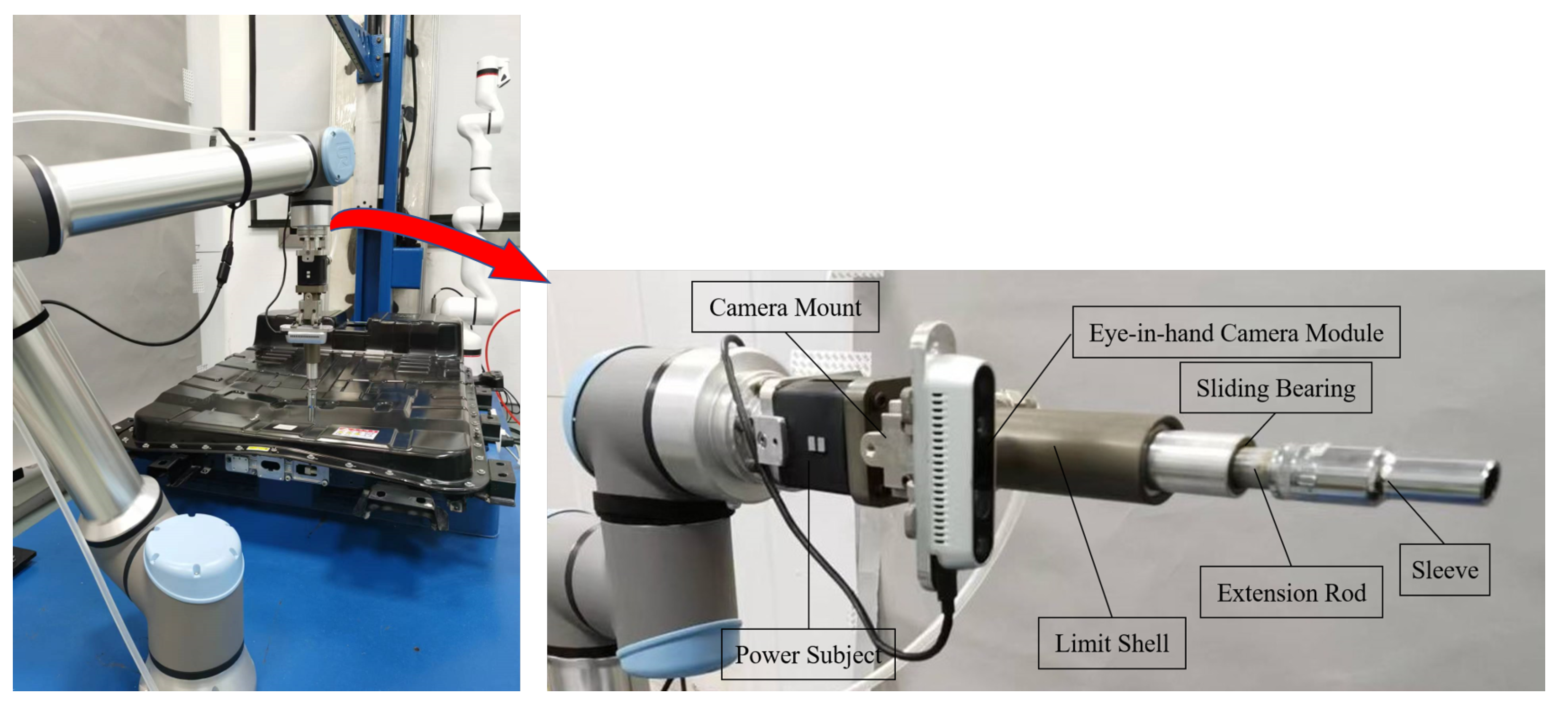
Our hardware platform is as shown in Figure 1.

We use a passive and compliant pneumatic torque actuator with vision sensing proposed by Zhang H. W. et al. [16] for the experiment (Figure 1). Information on some parameters of the robotic arm is shown in

Table 1. Information on some parameters of the robotic arm.

Item	Parameter
Robot type	UR10e
Eye-in-hand camera	Realsense D435
Weight	33.3 kg/73.5 lb
Maximum payload	10 kg/22 lb
Extension	1300 mm/57.2 in
Range of joints	$\pm 360$${}^{\circ }$ for all joints
Torque sensor accuracy	5.5 N
Degree of freedom	6 rotating joints
System update frequency	500 Hz

.

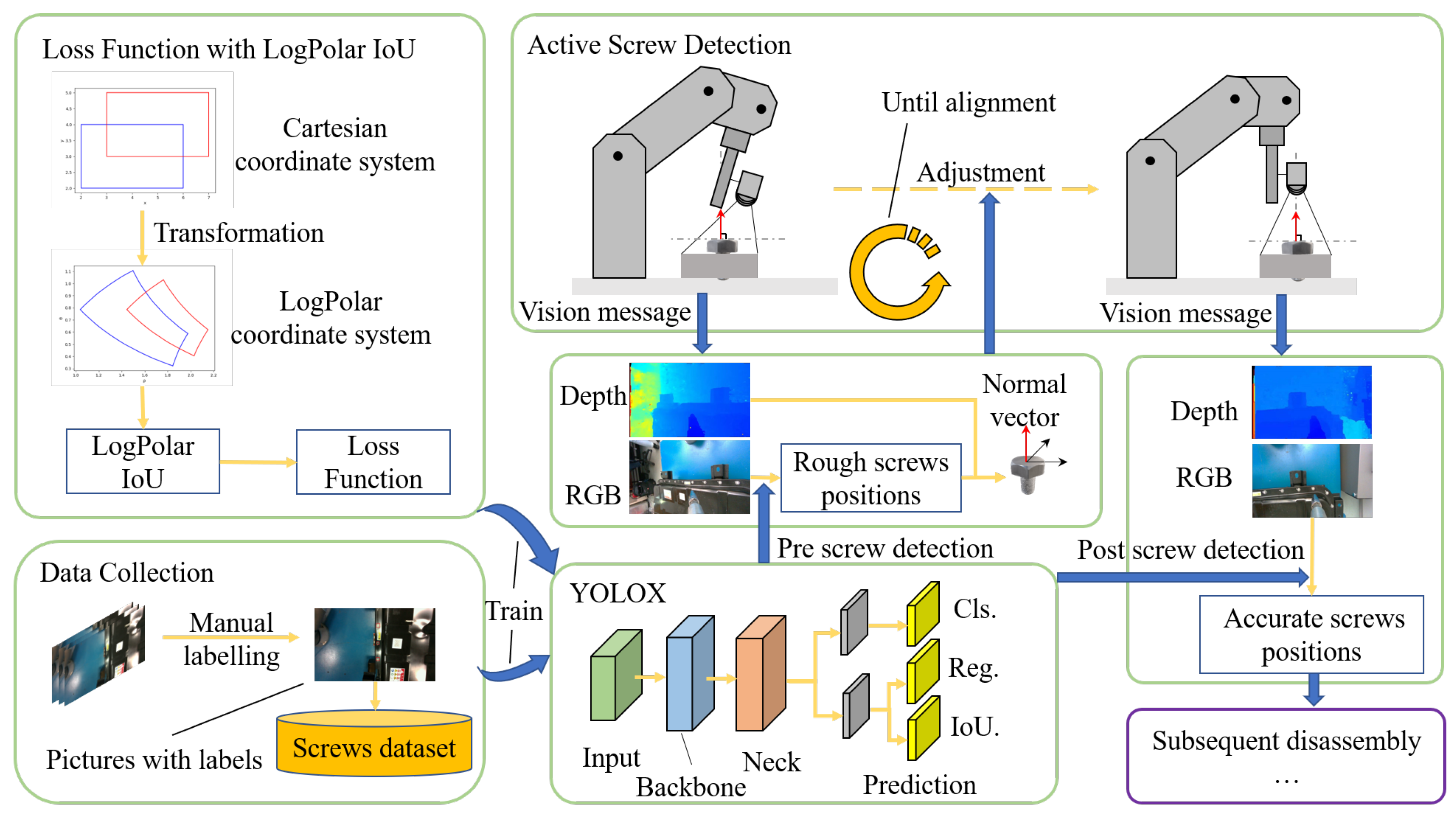
It mainly consists of a pneumatic power subject, a square shaft transmission limit module, a rod limit module, and an eye-in-hand camera module. Particularly, the eye-in-hand camera module includes a metal clamp and an Intel RealSense D435 camera, which can capture both RGB and depth images simultaneously. The “Active Screw Detection” process is shown in Figure 2. Firstly, the eye-in-hand camera module collects RGB and depth images of the robot arm in the initial position. Pre-screw detection is performed on the RGB image using a modified YOLOX model. The approximate pixel position of the screw is obtained. The normal vector of the screw plane is then calculated based on the pixel position of the closest screw to the robot arm, combined with the corresponding depth of the depth image. Here, a RANSAC-based plane fitting algorithm is proposed to calculate the normal vector of the target screw in order to minimise the effect of noise in the depth image. We can then control the robot arm to move to the optimal screw detection position, which is aligned with the normal vector of the target screw. In fact, due to the inherent unevenness of the screw surface and the noise in the depth image, moving to the optimal screw detection position is a process of gradual convergence. The system will continually check that the current position is the best observed position until the error is less than expected. At this point, the eye-in-hand camera module captures the image that is most suitable for screw detection. Post-screw detection is then performed based on the captured RGB images using the improved YOLOX model. The screw prediction box obtained at this point has a higher accuracy compared to the results of pre-screw detection. Finally, the exact spatial coordinates of the screw can be calculated based on the depth information of the corresponding area of the screw prediction box. In addition, compared to the native YOLOX model, this study proposes a LogPolar IoU loss function based on the Log Polar coordinate system to improve the training of the YOLOX model. The prediction box based on the Cartesian coordinate system is converted into a prediction box based on the Log Polar coordinate system. In order to avoid the problem of low convergence accuracy of the model due to the symmetry of the Cartesian coordinate system, the YOLOX model is trained using the self-labelled dataset with LogPolar IoU to make the convergence of the model more accurate. Higher detection and localisation accuracy is achieved.

2.1. Adaptive Adjustment of Robot Arm Angle

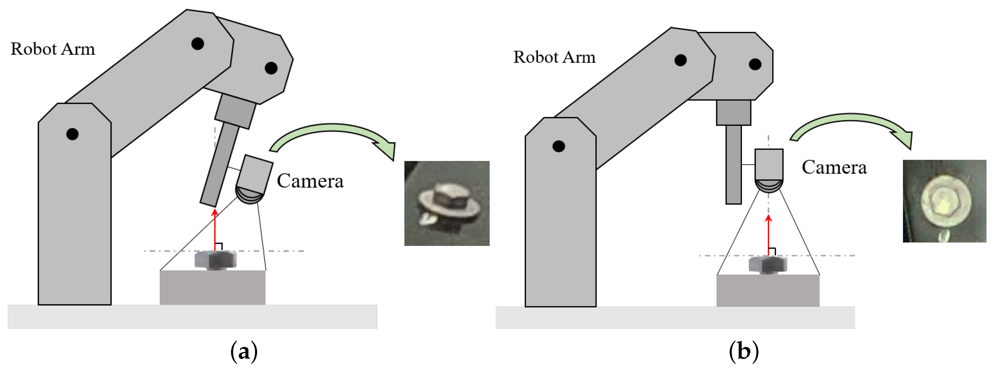
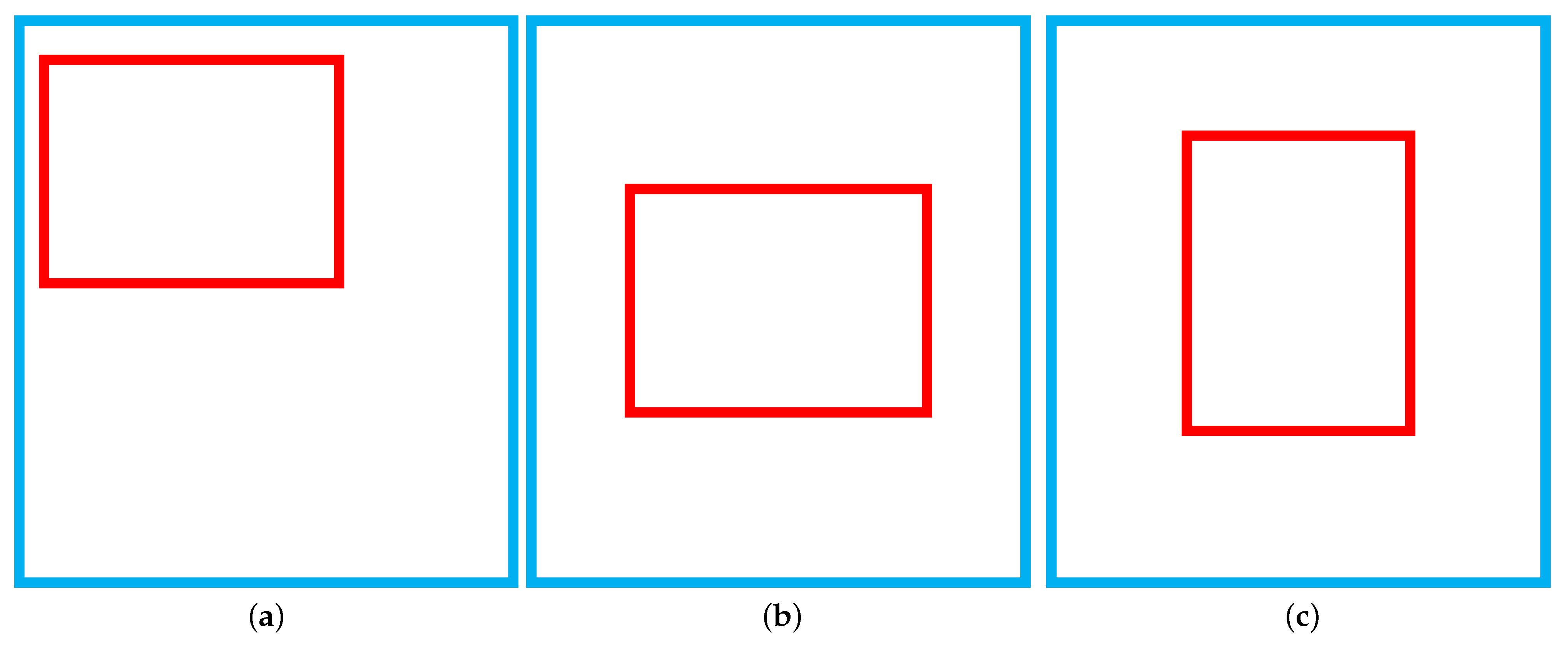
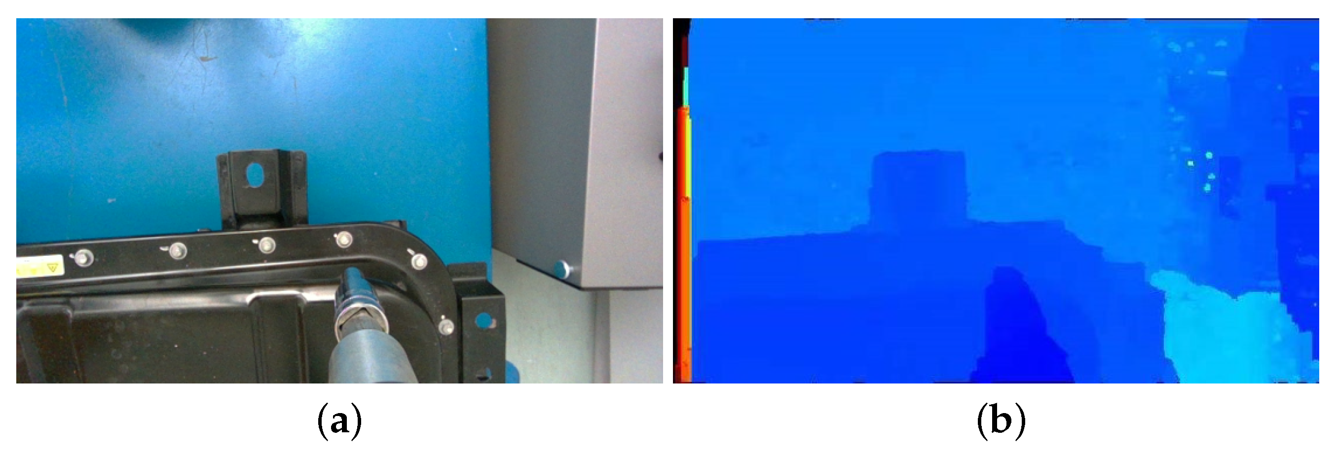
The target detection task for the screws is based directly on the RGB images captured by the vision sensor on the robotic arm. The information representation capability of the RGB images is limited by the angle at which the vision sensor is captured. For the screw with too large an angle between the normal vector of the upper surface and the vision sensor, Figure 3a, its main features are obscured, making it difficult to identify and localize the model. For the screw whose upper surface is approximately perpendicular to the capture angle of the vision sensor, on the other hand, the entire screw is clearly characterized, and the model is able to identify and localize it well during the detection process with a high confidence level for the foreground, Figure 3b.

In the screw disassembly task, the screw top layer of nuts is of a certain thickness, and the screw spacing between some automotive battery pack screws is not large. The excessive tilt angle of the visual sensor will, on the one hand, cause the screws to block each other or the washers, a feature-rich component, which is not conducive to the detection and positioning of the screws and can easily cause missed detection. On the other hand, the existence of the tilt angle will cause visual deformation of the screw, which in turn will have a greater impact on the accuracy of the screw classification and positioning. In the intelligent disassembly process of battery pack screws, the mechanical arm is constantly moving, which will cause the screw angle in the image collected by the vision sensor to vary greatly, thus affecting the positioning accuracy of the screw. Therefore, before the accurate positioning of the screws, the angle of the vision sensor needs to be corrected, which requires the mechanical arm to adjust the angle adaptively.

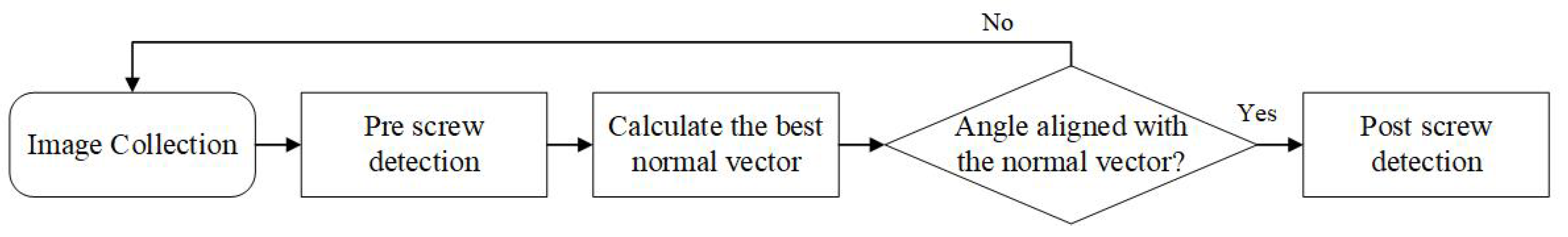
This study proposes an adaptive adjustment algorithm for the robotic arm based on the RANSAC algorithm to correct the attitude of the robotic arm so that it is in an attitude favorable to the screw detection and positioning task, see Figure 4. For the robotic arm that is performing the screw disassembly task, pre-screw detection is performed on its captured images. The best normal vector perpendicular to the screw to be disassembled is then calculated using the RANSAC algorithm. Finally, the robotic arm is paired with the best normal vector to adjust the pose of the robotic arm to the best pose for subsequent post-screw detection.

2.1.1. Acquisition of Plane Fitting Point Set

For the RGB map in the initial pose, the improved YOLOX model is used for pre-screw detection to obtain the set of prediction boxes of the screws, $S_{box}=\{b_1,b_2,\dots ,b_n\}$, to determine the approximate position of the screws, where each prediction box b contains the position information of the screw pixel points in the image. Then, the nearest prediction box $b_{min}$ to the robotic arm is obtained from $S_{box}$. The general scenario of $b_{min}$ is shown in Figure 5. Finally, the set of depth information corresponding to a certain number of pixel points, $S_{points}=\{d_1,d_2,\dots ,d_m\}$, is filtered from $b_{min}$. $S_{points}$ is the set of points used for plane fitting.

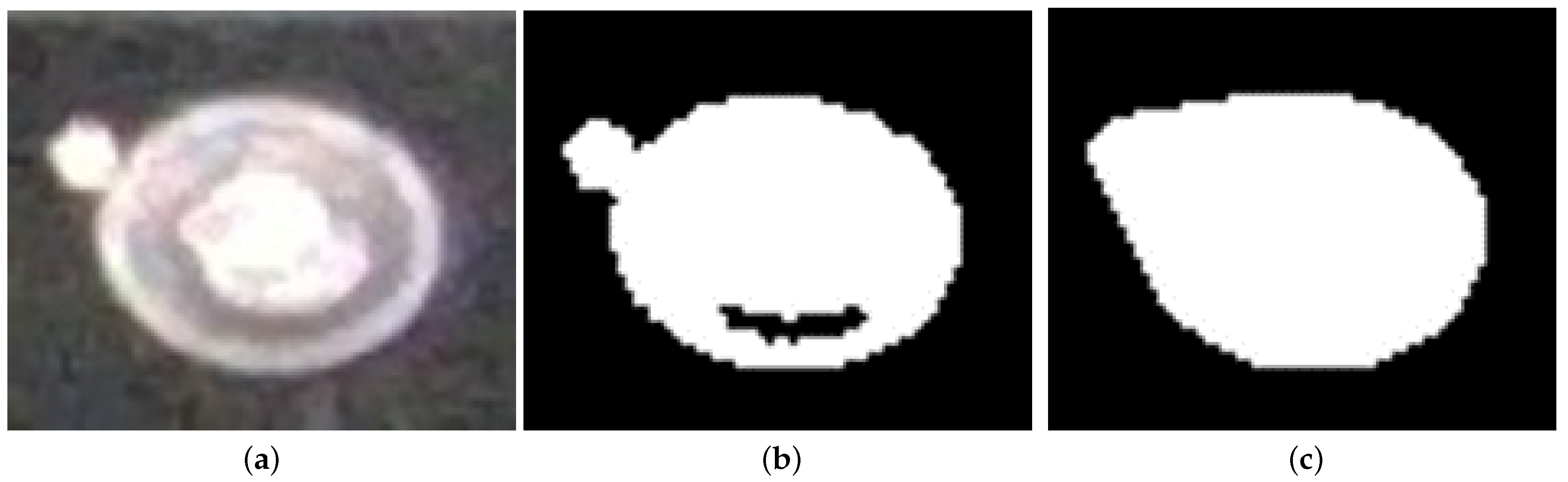
At the beginning of the experiment, we only selected a small number of random points in $b_{min}$ for plane fitting and found that the results were not satisfactory. The reason is that the points on the upper surface of the head are not in the same plane as the points in the background part, resulting in a large randomness in the fitted plane. Moreover, there are some noise points in the image captured by the vision sensor, and the plane fitted by selecting only a small number of points will be affected by the noise points. Therefore, it is necessary to use as many points as possible and in the same plane for plane fitting. Considering that the washer and nut of the screw itself are not in the same plane, the points of the screw part in prediction box $b_{min}$ are not suitable for plane fitting. However, the points of the background part are different, and they are generally in the same plane, which is suitable for plane fitting. In this study, the OTSU-based [46,47] binary thresholding method was used to split the screw part and the background part in $b_{min}$. The depth information corresponding to all the pixel points in the background part is selected to form $S_{points}$.

2.1.2. Ransac Algorithm for Plane Fitting

The RANSAC (Random Sample Consensus) algorithm is an iterative algorithm that correctly estimates the parameters of a mathematical model from a set of noisy data, and it is an uncertain algorithm that produces results with only one probability, which increases with the number of iterations. It divides the data into two sets of “outer points” and “inner points”. The “outer points” generally refer to noisy data in the data, such as false matches in matching and outliers in estimation curves and are used in plane fitting tasks to represent points that are far from the fitted plane. The “inner points” refer to the data that make up the model parameters, as opposed to the “outer points”. The RANSAC algorithm for plane fitting is shown in Algorithm 1.

Algorithm 1 RANSAC algorithm for plane fitting

Require: $S_{points}=p_1,p_2,\dots ,p_m$ is the set of all points used to fit the plane $P=0.99$ is the base probability of expecting RANSAC to get the model right $n_{limit}$ is the threshold at which the ‘inner point’ is expected $iterators=0$ indicates the number of iterations $v_{best}^T$ and $v^T$ are normal vector Ensure: $v^T$ is the plane normal vector obtained from the plane fit 1: while  $(n_{nliners}>n_{limit})or(iterators>k)$do 2:    random select n points from $S_{point}$ to build $S^{\prime }$ 3:    Calculate $v^T$ based on $S^{\prime }$ 4:    Calculate $n_{inliners}$ in $S_{points}$ 5:    Update the best plane normal vector $v_{best}^T$ and $n_{inliners}$ 6:    $t=n_{inliners}/(n_{inliners}+n_{outliners})$ 7:    $k=log(1-P)/log(1-t^n)$ 8:    $iterators=iterators+1$ 9: end while 10: return  $v_{best}^T$

For each iteration of the RANSAC algorithm, firstly, n points are randomly selected from $S_{points}$ to form a subset $S^{\prime }$, and a plane is fitted based on $S^{\prime }$ using the least squares method. Then, all the points of $S_{points}$ are divided into “inner points” and “outer points” by calculating the distance from the points to the plane and calculating the proportion t of “inner points”, Equation (1).

$$t=\frac{n_{inliners}}{n_{inliners}+n_{outliners}}$$

(1)

where $n_{inliners}$ denotes the number of interior points, and $n_{outliners}$ denotes the number of exterior points. Then, the probability that there is at least one “outliner” among the n randomly selected points in each iteration is $1-t^n$. Further, ${(1-t^n)}^k$ is the probability that at least one “outliner” is sampled in each of the k iterations of the fitting plane, then the probability that at least one “outliner” can be sampled is $1-t^n$. The probability of sampling only n “inner points” is $1-{(1-t^n)}^k$, Equation (2).

$$P=1-{(1-t^n)}^k$$

(2)

The desired number of iterations k for each iteration can be derived from this, as shown in Equation (3). However, it is not completely guaranteed that all points selected each time are “interior points”, and we can only expect P to be as close to 1 as possible, which is 0.99 in this study.

$$P=\frac{log(1-P)}{log(1-t^n)}$$

(3)

There are two conditions for the finalization of the RANSAC algorithm. One condition is that the number of “interior points” in the plane based on the current computation reaches $n_{limit}$, and the other condition is that the number of iterators exceeds the current desired number of iterations k.

After executing the RANSAC algorithm, the best plane normal vector $v_{best}^T$ corresponding to $S_{points}$ is obtained. Finally, the robotic arm adjusts its pose to match $v_{best}^T$ to achieve the best pose for the subsequent post-screw detection task.

2.1.3. Total Least Square for Plane Fitting

During each iteration of the RANSAC algorithm, the overall least squares method is used to compute the plane for a subset $S^{\prime }$ of $S_{points}$. Assume that the unit normal vector of the plane is $v^T=\left[\begin{array}{ccc}a& b& c\end{array}\right]$, Equation (4).

$$a^2+b^2+c^2=1$$

(4)

Suppose $(x_0,y_0,z_0)$ is any point in the desired plane.Then, the plane can be constructed by the point normal formula, Equation (5).

$$a(x-x_0)+b(y-y_0)+c(z-z_0)=0$$

(5)

Based on the calculated plane, the distance of all points of the set $S^{\prime }$ to the plane is calculated, which is the error of this plane fitting. Based on the fact that the distance from any point in space to the plane is equal to the projection on the normal vector of the vector composed of any point on the plane, the error is Equations (6) and (7).

$$J_2=\sum _{i=1}^n{d}_i^2=\sum _{i=1}^n\frac{{\left[(x-x_0,y-y_0,z-z_0)(a,b,c)\right]}^2}{a^2+b^2+c^2}$$

(6)

$$J_2=\sum _{i=1}^n{[a(x-x_0)+b(y-y_0)+c(z-z_0)]}^2$$

(7)

where $(x_i,y_i,z_i)$ denotes the i-th point in S’, and $d_i$ denotes the error distance of the i-th point to the plane. Then, the $J_2$ at this time is certainly the smaller the better. Then, you need to find the extreme value of $J_2$. $J_2$ calculates the partial derivatives of $x_0$, $y_0$, $z_0$, respectively, Equations (8)–(13).

$$\frac{\partial J_2}{\partial x_0}=2a\sum _{i=1}^n[a(x-x_0)+b(y-y_0)+c(z-z_0)]=0$$

(8)

$$\frac{\partial J_2}{\partial x_0}=2a[a(\overline{x}-x_0)+b(\overline{y}-y_0)+c(\overline{z}-z_0)]=0$$

(9)

$$\frac{\partial J_2}{\partial y_0}=2b\sum _{i=1}^n[a(x-x_0)+b(y-y_0)+c(z-z_0)]=0$$

(10)

$$\frac{\partial J_2}{\partial y_0}=2b[a(\overline{x}-x_0)+b(\overline{y}-y_0)+c(\overline{z}-z_0)]=0$$

(11)

$$\frac{\partial J_2}{\partial z_0}=2c\sum _{i=1}^n[a(x-x_0)+b(y-y_0)+c(z-z_0)]=0$$

(12)

$$\frac{\partial J_2}{\partial z_0}=2c[a(\overline{x}-x_0)+b(\overline{y}-y_0)+c(\overline{z}-z_0)]=0$$

(13)

where $\overline{x}$, $\overline{y}$, $\overline{z}$ denote the average of the three dimensional coordinates of all points in the set $S^{\prime }$, respectively. From Equations (9), (11), and (13), we know that the value of all partial derivatives is 0 when $x_0=\overline{x}$, $y_0=\overline{y}$, and $z_0=\overline{z}$, $J_2$ obtains the extreme value, and $J_2$ at this time is Equation (14).

$$J_2=\sum _{i=1}^n{[a(x_i-\overline{x})+b(y_i-\overline{y})+c(z_i-\overline{z})]}^2$$

(14)

Decompose $J_2$ into matrix multiplication according to Equation (14) to obtain Equations (15) and (16).

$$J_2=v^{T}Sv$$

(15)

$$S=\left[\begin{array}{ccc}\sum {(x-\overline{x})}^2& \sum (x_i-\overline{x})(y_i-\overline{y})& \sum (x_i-\overline{x})(z_i-\overline{z})\\ \sum (x_i-\overline{x})(y_i-\overline{y})& \sum {(y_i-\overline{y})}^2& \sum (y_i-\overline{y})(z_i-\overline{z})\\ \sum (x-\overline{x})(z_i-\overline{z})& \sum (y_i-\overline{y})(z_i-\overline{z})& \sum {(z-\overline{z})}^2\end{array}\right]$$

(16)

where $v^T=\left[\begin{array}{ccc}a& b& c\end{array}\right]$ is the normal vector of the plane obtained from this subplane fit. It can be found that the matrix S is a positive definite matrix. Then, it can be decomposed into Equation (17).

$$S=\left[\begin{array}{ccc}{q}_1& q_2& q_3\end{array}\right]\left[\begin{array}{ccc}{\lambda }_1& & \\ & {\lambda }_2& \\ & & {\lambda }_3\end{array}\right]\left[\begin{array}{c}{q}_1\\ q_2\\ q_3\end{array}\right]=Q\mathsf{\Lambda }{Q}^T$$

(17)

where the matrix Q is composed of the eigenvectors of the matrix S, and ${\lambda }_1$, ${\lambda }_2$, ${\lambda }_3$ are the eigenvalues of the matrix S. Equation (18) can be derived from Equations (16) and (17).

$$J_2=v^{T}Q\mathsf{\Lambda }{Q}^{T}v=\left(v^{T}Q\right)\mathsf{\Lambda }{\left(v^{T}Q\right)}^T$$

(18)

Define Equation (19):

$$u_1=v^T{q}_1,u_2=v^T{q}_2,u_3=v^T{q}_3,U^T=\left[\begin{array}{ccc}{u}_1& u_2& u_3\end{array}\right]$$

(19)

Equation (19) is brought into Equation (18) to obtain Equation (20).

$$J_2=U^T\mathsf{\Lambda }U=\left[\begin{array}{ccc}{u}_1& u_2& u_3\end{array}\right]\left[\begin{array}{ccc}{\lambda }_1& & \\ & {\lambda }_2& \\ & & {\lambda }_3\end{array}\right]\left[\begin{array}{c}{u}_1\\ u_2\\ u_3\end{array}\right]$$

(20)

Equation (20) was further calculated to obtain Equation (21).

$$J_2={\lambda }_1{u}_1^2+{\lambda }_2{u}_2^2+{\lambda }_3{u}_3^2$$

(21)

In addition, because:

$$U^{T}U=v^{T}Q{\left(v^{T}Q\right)}^T=v^{T}Q{Q}^{T}v=v^{T}v=E$$

(22)

From Equation (22), matrix U is the unit vector, Equation (23).

$$u_1^2+u_2^2+u_3^2=1$$

(23)

It may be set ${\lambda }_1\le {\lambda }_2\le {\lambda }_3$, then Equations (21)–(23) can be further calculated according to the inequality to obtain Equation (24).

$${\lambda }_1={\lambda }_1(u_1^2+u_2^2+u_3^2)\le J_2\le {\lambda }_3(u_1^2+u_2^2+u_3^2)={\lambda }_3$$

(24)

From Equation (24), the minimum value of $J_2$ is ${\lambda }_1$, when $u_1=1$, $u_2=u_3=0$. From Equation (19), $v=q_1$. In summary, when $v=q_1$, the error value $J_2$ takes the minimum value ${\lambda }_1$, where ${\lambda }_1$ is the minimum eigenvalue of the matrix S, and $q_1$ is the eigenvector corresponding to ${\lambda }_1$. Here, $q_1$ can be quickly calculated by matrix singular value decomposition. Constructing the matrix A from the set $S^{\prime }$, see Equation (25), it is easy to find that $A^{T}A=S$. Since $q_1$ is the eigenvector corresponding to the smallest eigenvalue of the matrix S, then $q_1$ is the eigenvector corresponding to the smallest eigenvalue of the matrix $A^{T}A$.

$$A=\left[\begin{array}{ccc}{x}_1-\overline{x}& y_1-\overline{y}& z_1-\overline{z}\\ x_2-\overline{x}& y_2-\overline{y}& z_2-\overline{z}\\ ...& ...& ...\\ x_n-\overline{x}& y_n-\overline{y}& z_n-\overline{z}\end{array}\right]$$

(25)

The singular value decomposition of the matrix A is shown in Equation (26).

$$A=U\Sigma V^T$$

(26)

where the matrix V consists of eigenvectors of the matrix $A^{T}A$, and each column of eigenvectors from left to right corresponds to the eigenvalues in decreasing order. Then, the eigenvector corresponding to the smallest eigenvalue is the last column of the matrix V, which corresponds to the last row of the matrix $V^T$. Then, $q_1$ is the last row of matrix $V^T$, and the normal vector $v^T$ of the plane constructed by the set $S^{\prime }$ can be found quickly.

2.2. Screw Detection Based on YOLOX Model

Active Screw Detection uses the improved YOLOX model proposed in this study for screw detection. The implementation principle of the YOLOX model and the network structure are described in detail in the subsequent sections of this subsection.

2.2.1. Architecture of YOLOX Model

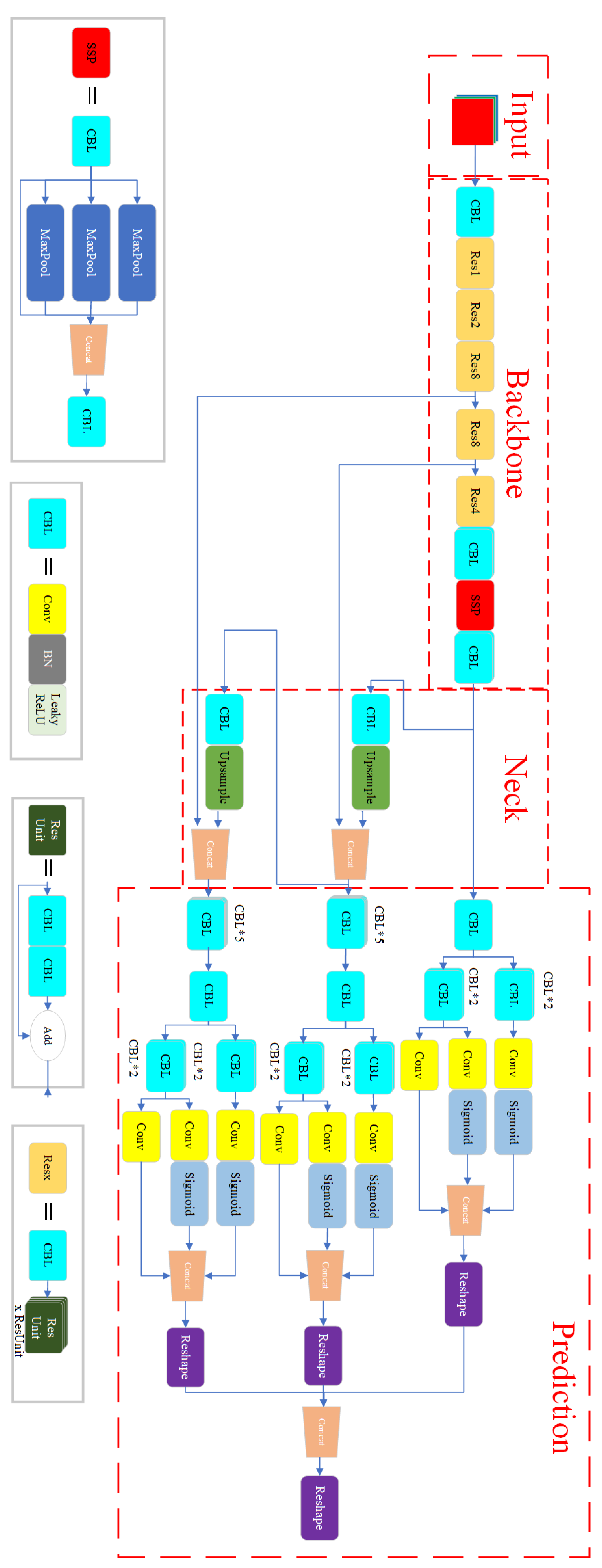
The YOLOX model [23] is used to detect and locate the screws based on the RGB image captured by the vision sensor. Its role is to obtain information about the coordinates of the pixel region where each screw is located in the RGB image. YOLOX is a neural network model for deep learning. The main principle is to use a neural network to extract feature information from the RGB image and then use operations, such as decoupling and convolution, to obtain prediction boxes. These prediction boxes frame the area where the screws are located. The YOLOX model consists of four parts: Input, BackBone, Neck, and Prediction, and the specific network structure is shown in Figure 6. RGB images captured by vision sensors are used as input to YOLOX, and pre-processing is performed at the input. Then, BackBone performs feature extraction on different images fine-grained for the preprocessed images. Then, Neck obtains the features under different perceptual fields and converts the extracted feature information into coordinates, categories, and other information. Finally, the Prediction part is decoupled to obtain the position information, category, and confidence of the detected boxes, respectively.

2.2.2. Input

In the Input section, a preprocessing operation is performed on the RGB images to unify the size of the input images. In addition, high-resolution images contain too much pixel information to be used directly for neural network calculations that would take up a large amount of GPU video memory. To reduce the performance requirements of the model on the hardware, the images are scaled and filled. In the training phase of the model, the RGB images in the dataset are enhanced with Mosaic and MixUp data to expand the quantity and quality of the dataset. The Mosaic data enhancement method, which was applied in the YOLOv3 model, has proved to be beneficial to model learning and training. The Mosaic data augmentation method stitches the calibrated RGB images by random scaling, random cropping, and random arrangement to expand the dataset and the diversity of images in the dataset. The Mosaic method is an additional enhancement strategy, which randomly selects two images for scaling, filling, and merging and then sets a fusion factor for the respective labels of the images to generate a new label. This module turns off the data enhancement method after the model training is finished.

2.2.3. BackBone

The BackBone part is consistent with YOLOv3 and uses the DarkNet53 network model [21], which is a classical deep network mainly composed of residual convolution and SPP modules. The residual convolution consists of convolutional layer jump connections, whose role is to extract the feature information in the input image. The structure of the residual avoids the problems of gradient explosion and gradient disappearance caused by too deep layers of the network. In the middle of the residual module, a convolutional layer with a kernel of 3 × 3, a step size of 2 and a padding of 1 is added to downsample and upgrade the output feature map of each residual block. The SPP structure mainly consists of maximum pooling layers of different sizes, and the feature maps after downsampling of different sizes are stitched together to obtain richer texture features, which is beneficial to the subsequent detection operations.

2.2.4. Neck

The Neck part consists of an FPN structure, a pyramid-shaped feature extraction module. Its function is to extract shallow features, middle features, and high features obtained from the convolution of different depth residuals in the BackBone part and construct three feature maps based on different perceptual fields of the original image using convolution and upsampling operations from top to bottom. This part mainly focuses on the different sizes of screws with different percentages in RGB pictures, which is equivalent to the average chunking of the original picture in three sizes and carries out the subsequent screw detection localization classification task based on the regions of these three sizes. In the screw disassembly process, the height of the robotic arm will constantly change, which will lead to a large difference in the proportion of the same screw in the pictures collected by the vision sensor, and the use of FPN structure can effectively ensure the accuracy of subsequent screw identification and localization.

2.2.5. Prediction Head

Unlike the network structure of the previous YOLO series, YOLOX performs a decoupling operation in the Prediction Head part to calculate the classification task and the regression task separately. The conflict between classification and regression tasks is a very common problem because during the final convolution operation, the convolution kernel parameters are shared, which leads to the feature maps containing both tasks affecting each other. By separating the feature maps of classification and regression tasks, this problem can be avoided and the accuracy of classification and localization can be improved. SimOTA in the Prediction Head section obtains and filters the positive sample prediction boxes. The anchor-based approach is used in the network before YOLOv5 to obtain the prediction boxes. The k-means algorithm was used to cluster the sizes of the ground-truth boxes in the dataset, and the sizes of the centroids of the nine categories were taken as the sizes of the prior bounding boxes. The prior bounding boxes of 9 sizes are assigned to the feature maps of 3 sizes of perceptual fields obtained from the BackBone and Neck parts. Then, each cell under each size of perceptual field corresponds to 3 sizes of prior bounding boxes. The role of the prior bounding box is to give an initial value to the prediction box. The output of the model represents the box centroid and the offset of the width and height. The mapping relationship is used to combine the prior bounding boxes and the model output to obtain the final prediction boxes. In the anchor-based approach, each cell is responsible for three sizes of a prior bounding boxes, which depend on the ground-truth box size of the labels in the dataset, making it difficult to guarantee the generalization of the model.The YOLOX anchor-free approach generates prediction boxes directly based on each feature point using the feature maps of the three size senses. The advantage of this is that the generated prediction boxes do not depend on the ground-truth boxes information of the labels in the dataset, avoiding the limitation in terms of data. The number of ground-truth boxes is much smaller than these directly generated prediction boxes, so it is also necessary to select the positive sample prediction boxes among them, and SimOTA is used here. First, the cost matrix between each ground-truth box and each prediction box is calculated, see Equation (27).

$$cos{t}_{ij}=L_{ij}^{cls}+{\lambda }_1{L}_{ij}^{reg}+{\lambda }_2{L}_{ij}^{cen}$$

(27)

where ${\lambda }_1$ and ${\lambda }_2$ are balance coefficients, i and j are subscripts, $L_{ij}^{cls}$ is the classification loss of each ground-truth box and the current feature point prediction box, $L_{ij}^{reg}$ is the position loss of each ground-truth box and the current feature point prediction box, and $L_{ij}^{cen}$ is whether the center of each ground-truth box falls within a certain radius of the feature point. The IoU of each ground-truth box is calculated and rounded down to obtain $dynami{c}_k$. The first $dynami{c}_k$ boxes with the lowest cost are taken as the positive samples of the ground-truth box, and the rest are all negative samples. YOLOX uses this method together with anchor-free to filter the prediction boxes, which not only reduces the training time but also avoids additional parameters compared to the OTA used in YOLO.

2.2.6. Output of YOLOX

In the screw detection and localization task, the prediction results of $S\times S\times 7$ dimensions are generated under each perceptual field, where S × S denotes the number of cells into which the predicted image is divided, and each cell contains 7 channels of output, which consists of 3 branches, i.e., cls, obj, and reg branches. The cls branch occupies 2 channels to indicate which type of screw the object in the predicted detection box belongs to. The obj branch occupies 1 channel to distinguish whether the prediction box is foreground or background. The reg branch occupies 4 channels, including the location of the center point of the prediction box and the dimensions of the width and height.

2.2.7. Loss Function

The loss function of YOLOX is the sum of all losses averaged over the number of positive labels according to the output cls, obj, and reg branches, and its loss function is shown in Equation (28).

$$L=\frac{1}{N_{pos}}(L_{cls}+L_{obj}+{\lambda }_{reg}{L}_{reg})$$

(28)

where $N_{pos}$ is the number of positive samples obtained by SimOTA screening, ${\lambda }_{reg}$ is the balance coefficient, and $L_{cls}$ is the loss value of the classification task, whose cross-entropy loss is calculated for the classification results of the positive samples with the classification labels of the ground-truth boxes, as shown in Equation (29).

$$L_{cls}=-\sum _i^{N_{pos}}[t_{i}log\left(p_i\right)+(1-t_i)log(1-p_i)]$$

(29)

where $N_{pos}$ denotes the total number of samples, $t_i$ denotes the true label of each target, and $p_i$ denotes the predicted classification result. $L_{obj}$ is the confidence loss value, which is calculated as the cross-entropy for the confidence of all samples, see Equation (30).

$$L_{obj}=-\sum _i^N[c_{i}log\left({\widehat{c}}_i\right)+(1-c_i)log(1-{\widehat{c}}_i)]$$

(30)

where N is the number of samples, $c_i$ is the true confidence of each target, which is 1 for foreground and 0 for background, and ${\widehat{c}}_i$ is the confidence of each prediction box, which is not simply 1 or 0, but multiplied by the IoU of the prediction box and its corresponding ground-truth box. $L_{reg}$ is the regression loss value of the ground-truth boxes, which is obtained by calculating the IoU of the prediction box and its corresponding ground truth. Since in the paper presented by YOLOX, the authors only state that $L_{reg}$ is obtained by IoU and do not give a specific formula, we derived the formula for the $L_{reg}$ part from the open source source code, see Equation (31).

$$L_{reg}=1-Io{U}^2$$

(31)

The IoU represents the intersection ratio of the area of the prediction box and its corresponding ground-truth box, and its principle and calculation process will be elaborated in Section 2.3.

2.3. Logpolar IoU

In the training process of the regression task for target detection, how to obtain the loss value of the prediction box and the ground-truth box is the key step, and the common method is to use IoU and the improved version of IoU to perform the calculation.

2.3.1. IoU

Intersection over Union (IoU) is the original version of IoU, widely used in the field of target detection, which calculates the area intersection ratio of the prediction box to the ground-truth box, see Equation (32).

$$IOU=\frac{B\cap B^{gt}}{B\cup B^{gt}}$$

(32)

where $B^{gt}$ is the ground-truth box, B is the prediction box, $B\cap B^{gt}$ denotes the area of the intersection part of the prediction box and the ground-truth box, and $B\cup B^{gt}$ denotes the area of the merged part of the prediction box and the ground-truth box. Although IoU can visually represent the overlap of the two boxes, it also has some problems.

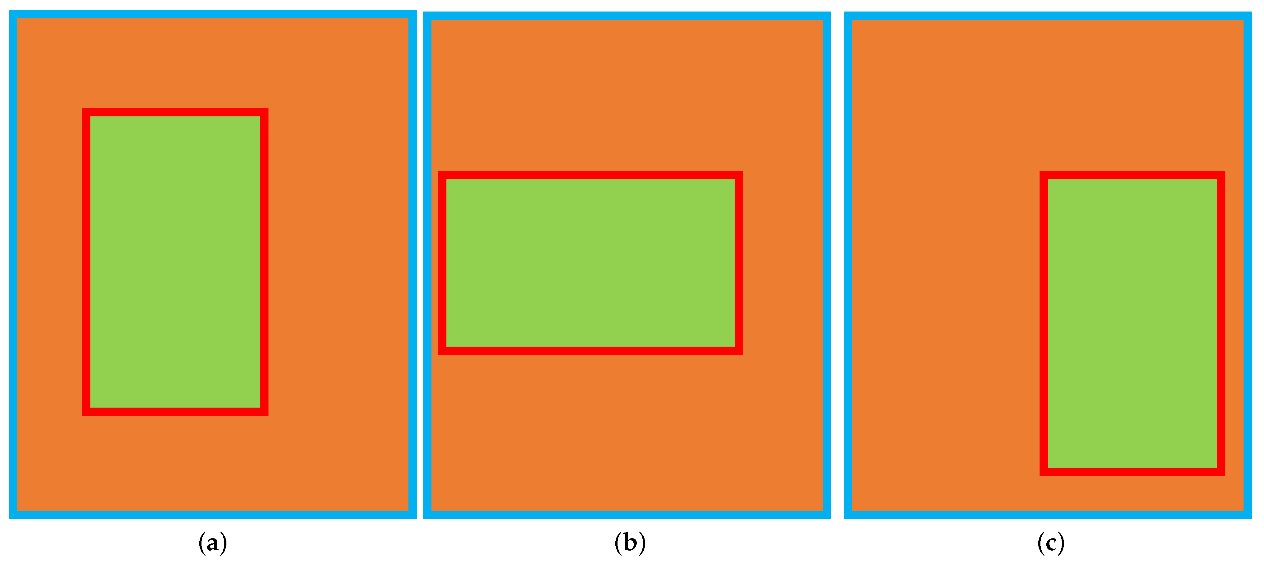
On the one hand, if there is no intersection between the prediction box and the ground-truth box, then the value of IoU will be zero, and it will be useless. When screening the positive samples, YOLOX will only keep the prediction box samples whose center point of the prediction box falls within a certain range of the center point of the ground-truth box so that the intersection of the prediction box and the ground-truth box will definitely exist, avoiding this defect of IoU. However, on the other hand, if one box is contained in another box, see Figure 7, and the area of both boxes remains the same, then the values of both $B\cap B^{gt}$ and $B\cup B^{gt}$ do not change, and the value of IoU does not change either, which eventually leads to the failure of this part to contribute to the training process. Subsequently, there are some versions of IoU that improve the original defects of IoU.

2.3.2. Improved Version of IoU

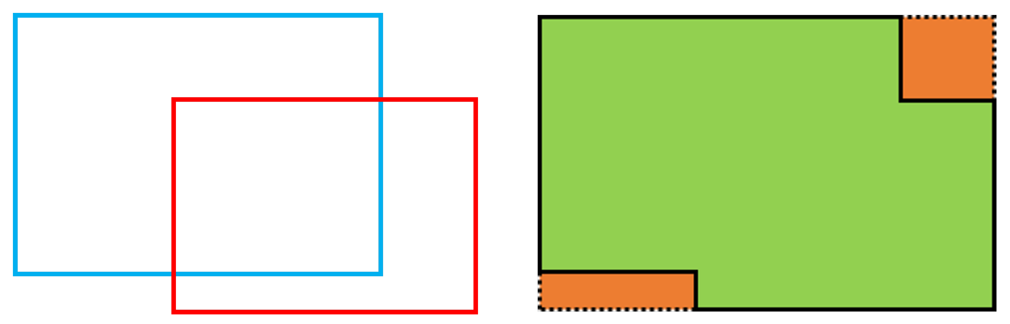
To solve the problem that a constant value of 0 for IoU does not contribute to the training process when there is no intersecting part between the prediction box and the ground-truth box, GIoU is proposed [48]. GIoU takes into account two factors, the area of the smallest box containing the prediction box and the detection box and the area of the non-prediction box and detection box area within the smallest box, see Equation (33).

$$GIoU=IoU-\frac{C-(B\cup B^{gt})}{C}$$

(33)

where $B^{gt}$ is the ground-truth box, B is the prediction box, C is the area of the smallest box that contains both the prediction box and the ground-truth box, $B\cup B^{gt}$ denotes the area of the part of the prediction box that merges with the ground-truth box, and then $C-(B\cup B^{gt})$ denotes the area of the non-prediction box and ground-truth box area within the smallest box, see Figure 8.

When the two boxes are very far apart, IoU loses its role by being constant at zero, and GIoU still provides a loss calculation through the relationship between the position of the boxes and their area. However, GIoU still does not solve the case where one box is contained within another, see Figure 9. In this case, $B\cup B^{gt}$ and $B\cap B^{gt}$ as well as C will remain constant, and the value of GIoU will remain constant, making no contribution to the training process.

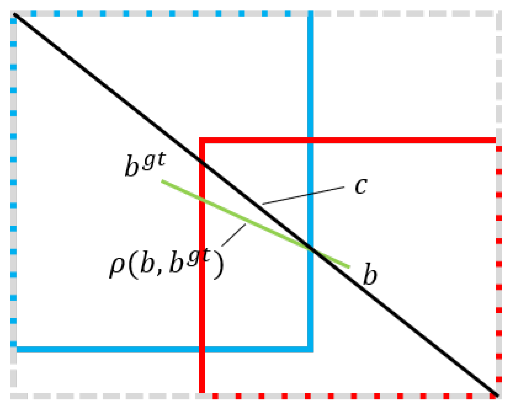
To address the fact that IoU and GIoU cannot handle the case where one box is contained in another, DIoU considers the ratio of the distance between the centre point of the prediction box and the detected box to the distance between the diagonals of the smallest box containing both boxes, Equation (34).

$$DIoU=IoU-\frac{{\rho }^2(b,b^{gt})}{c^2}$$

(34)

where $b^{gt}$ is the Cartesian coordinate of the centre point of the ground-truth box, b is the Cartesian coordinate of the centre point of the prediction box, $\rho (b,b^{gt})$ denotes the Euclidean distance between the prediction box and the midpoint of the ground-truth box, and c denotes the Euclidean distance of the diagonal of the smallest box that contains both the prediction and ground-truth boxes, see Figure 10.

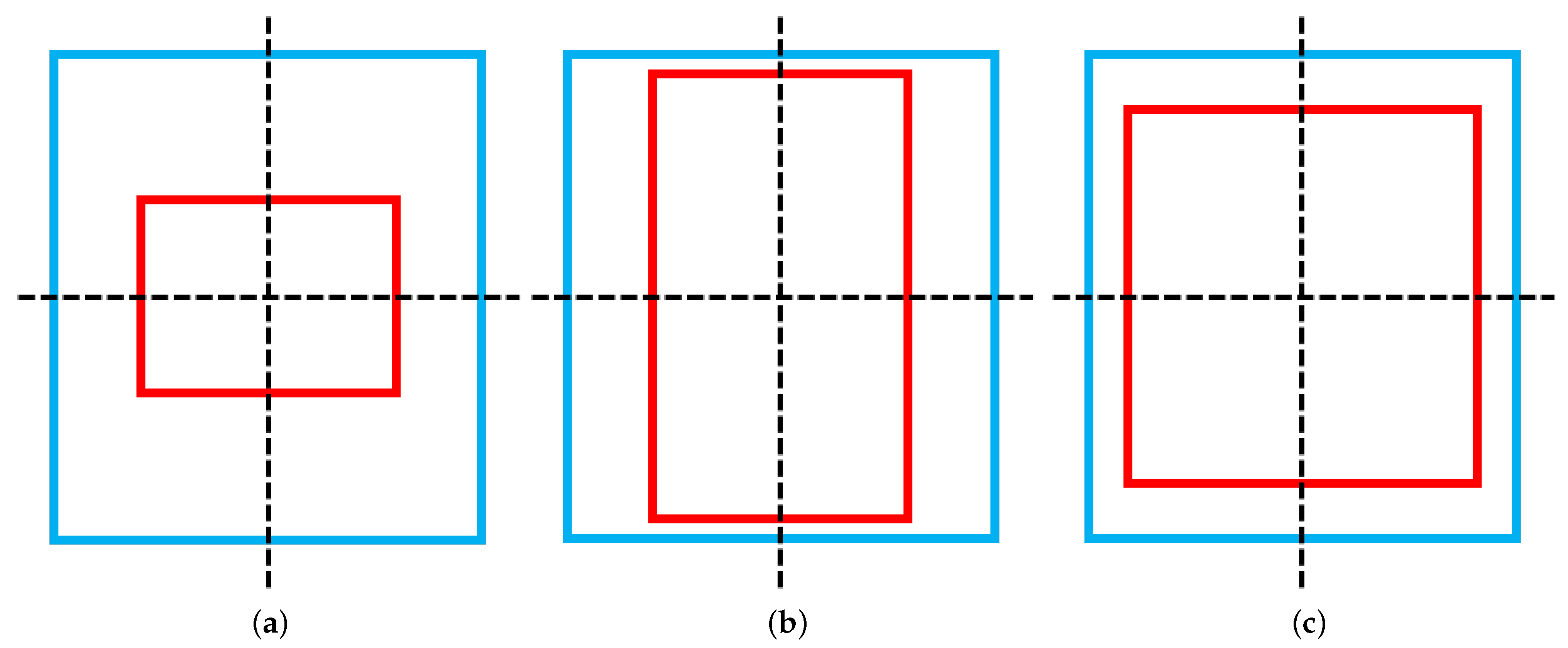
DIoU somewhat avoids the problem of degradation of the regression loss function as the model converges, while still providing loss for training when the prediction box is far away from the ground-truth box without an intersecting part. However, DIoU can fail in some cases. The DIoU degenerates into an IoU when the prediction box coincides with the centroid coordinates of the ground-truth box and one box is contained within the other, see Figure 11, where the value of $\rho (b,b^{gt})$ is 0. At this point, the DIoU is completely useless if the large box is left unchanged and the small box changes in width and height while keeping the area the same.

The authors of DIoU were also aware of this problem and subsequently proposed CIoU, which adds the aspect ratio of the prediction box to the ground-truth box as a penalty factor, see Equations (35)–(37).

$$CIoU=IoU-\frac{{\rho }^2(b,b^{gt})}{c^2}+\alpha v$$

(35)

$$v=\frac{4}{{\pi }^2}(\arctan \frac{w^{gt}}{h^{gt}}-\arctan \frac{w}{h})$$

(36)

$$\alpha =\frac{v}{(1-IoU)+v}$$

(37)

where $w^{gt}$ and $h^{gt}$ denote the width and height of the ground-truth box, w and h denote the width and height of the prediction box, respectively, v is used to measure the consistency of the aspect ratio, and $\alpha$ is the weight function. By taking the aspect ratio into account, CIoU compensates for the deficiency of DIoU scoring the same area at different scales. CIoU is also the loss function for the YOLOv5 model to calculate the difference between the prediction box and the ground-truth box.

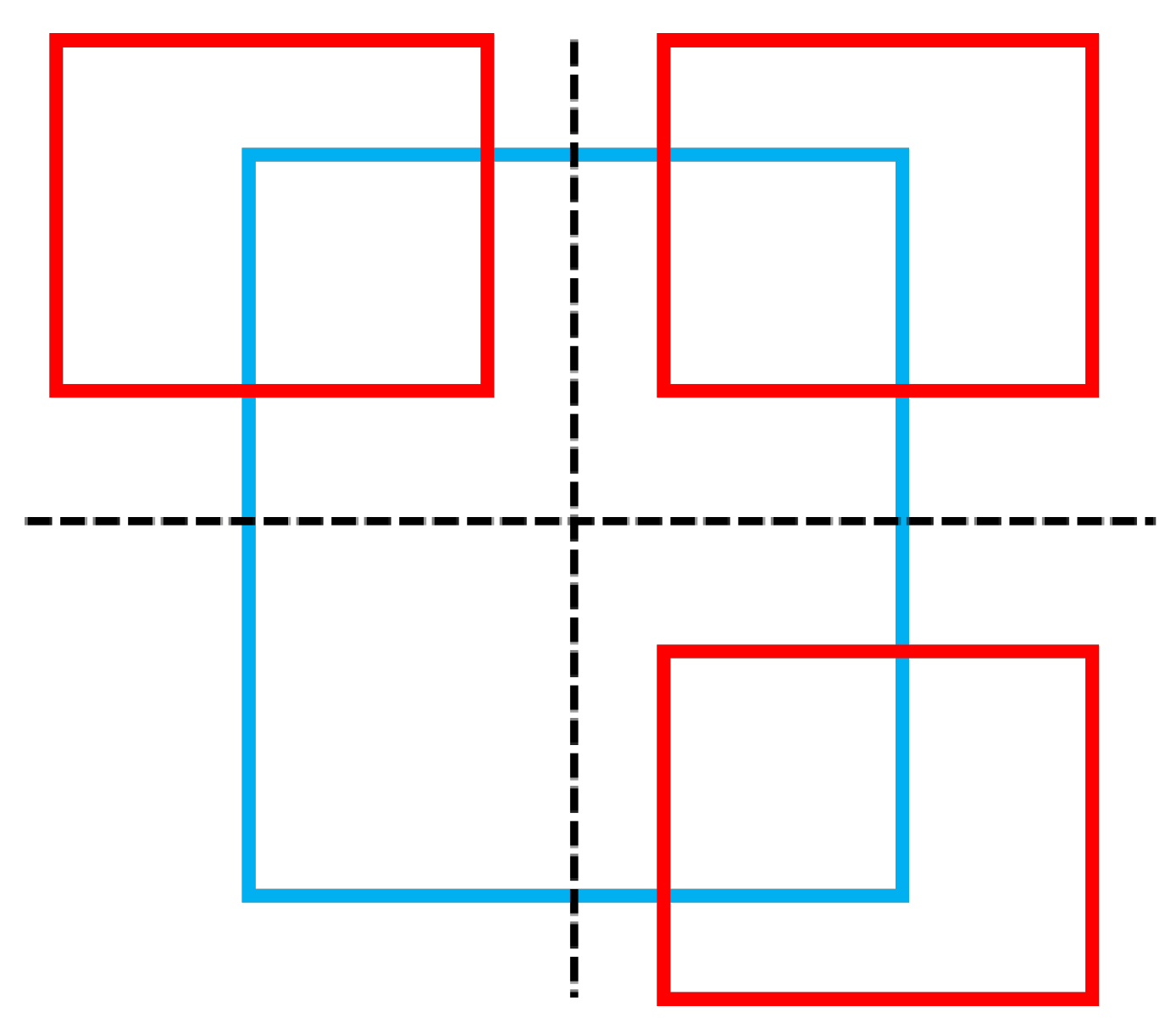
In the regression task, the loss value as a penalty term provides the direction of convergence for the training of the neural network model. During the training of the neural network, the position of the ground-truth box is constant, and the prediction box will gradually approach the ground-truth box as the training progresses and the loss value becomes progressively smaller. We would like the prediction box to return different loss values at different locations, which would facilitate the convergence of the neural network, as well as improve the detection accuracy. The current versions of IoU do not provide significant differences when calculating the loss of the detection box in the symmetric case, see Figure 12.

When the prediction box is very close to the ground-truth box, the neural network gradually converges and the step of the prediction box adjustment will gradually become smaller, which can easily move to a symmetrical position, thus making the effectiveness of the position loss function weaker and eventually affecting the localization accuracy. Therefore, this study proposes to convert the coordinates of the detection box in the Cartesian coordinate system into the Log Polar coordinate system and use the mode of the vector in the Log Polar coordinate system to calculate the loss instead of the Euclidean distance.

2.3.3. Logpolar IoU

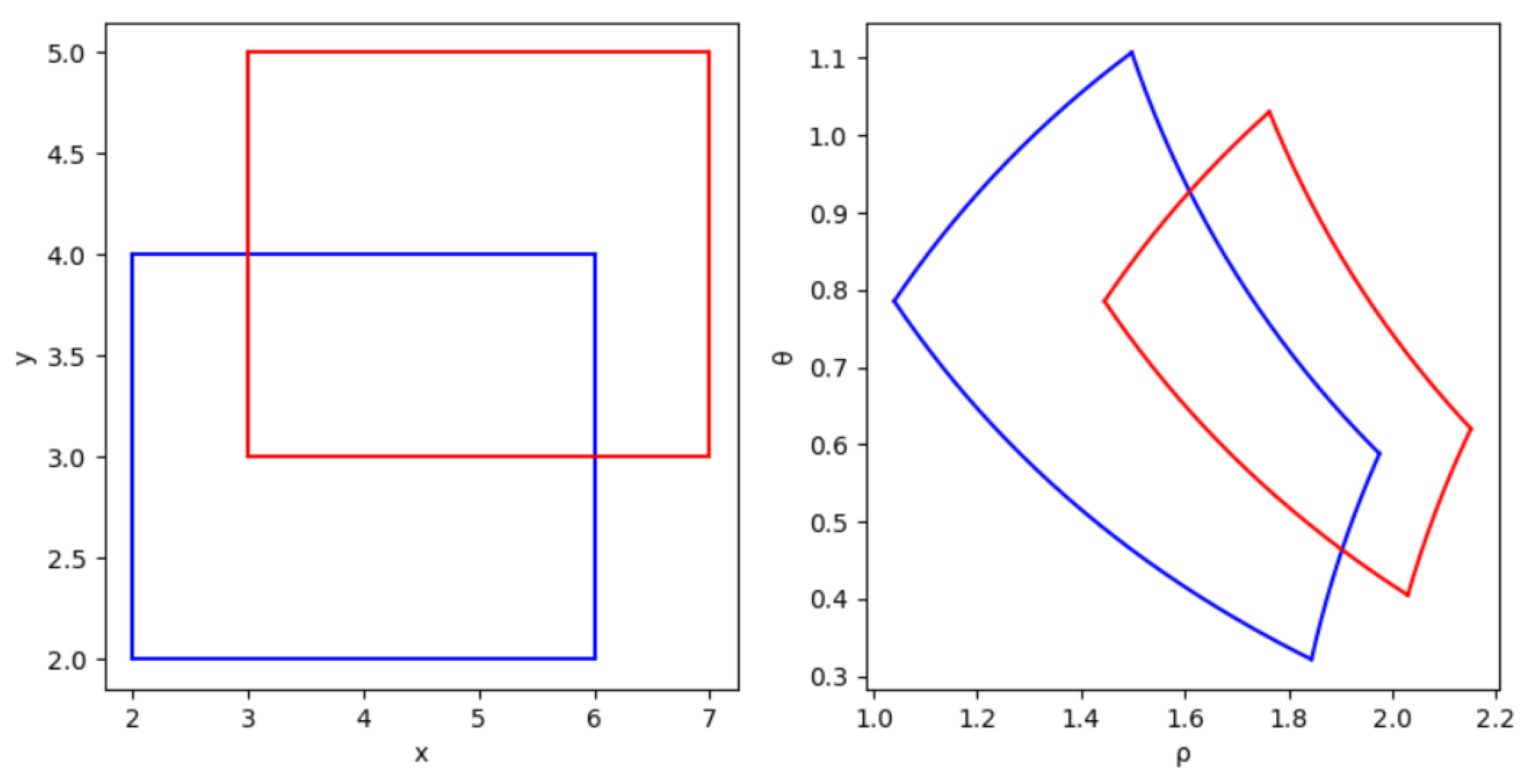
We assume that each pixel point on the image is a point in the Cartesian coordinate system and that information about the position and dimensions of the prediction and ground-truth boxes can be represented by Cartesian coordinates. A point $(x,y)$ in the Cartesian coordinate system is converted to the corresponding coordinate $(\rho ,\theta )$ in the Log Polar coordinate system, see Equations (38) and (39).

$$\rho =\sqrt{x^2+y^2}$$

(38)

$$\theta =\left\{\begin{array}{cc}\frac{\pi }{2}\hfill & if x=0andy>0\hfill \\ \arctan \left(\frac{y}{x}\right)\hfill & if x>0andy\ge 0\hfill \end{array}\right.$$

(39)

where $\rho$ denotes the polar diameter, and $\theta$ denotes the polar angle. As the image occupied only the first quadrant in the original Cartesian coordinate system, the value domain of $\theta$ was $[0,\frac{\pi }{2}]$. The prediction box is transformed from the ground-truth box through the coordinate system, see Figure 13.

In the Log Polar coordinate system, the distance between any two points is the vector modulus of the difference between the polar diameter and the polar angle, Equations (40)–(43).

$$\Delta \rho ={\rho }_1-{\rho }_2$$

(40)

$$\Delta \theta ={\theta }_1-{\theta }_2$$

(41)

$$\overrightarrow{\lambda }=(\Delta \rho ,\Delta \theta )$$

(42)

$$\left|\overrightarrow{\lambda }\right|=\sqrt{{(\Delta \rho )}^2+{(\Delta \theta )}^2}$$

(43)

where $({\rho }_1,{\theta }_1)$ and $({\rho }_2,{\theta }_2)$ denote the coordinates of any two points in the Log Polar coordinate system, and $\left|\overrightarrow{\lambda }\right|$ denotes the vector mode of the two points. The vector mode in the Log Polar coordinate system is used as the distance between the two points, replacing the distance in the Cartesian coordinate system in CIoU, thus enabling the prediction box in the symmetric case to produce different loss values at different locations and inducing more accurate convergence of the model; logPolar IoU is shown in Equation (44).

$$LogPolarIoU=IoU-\frac{{\rho }_{lp}^2(b,b^{gt})}{c_{lp}^2}+\alpha v$$

(44)

where ${\rho }_{lp}(b,b^{gt})$ denotes the vector mode of the centroid of the prediction box and the ground-truth box in the corresponding coordinates of the Log Polar coordinate system, $c_{lp}$ denotes the vector mode of the diagonal coordinates of the smallest box containing both the prediction box and the ground-truth box in the corresponding coordinates of the Log Polar coordinate system, and $\alpha$ and v continue to follow the penalty terms of the aspect ratio in CIoU.

The Log Polar coordinate system is equivalent to changing the viewing angle of the observation with respect to the Cartesian coordinate system. In the Cartesian coordinate system, the viewpoint is on the ground-truth box, and the prediction box passes through many symmetrical places as it keeps moving, producing the same losses and thus diminishing the effect of the loss function. In contrast, under the Log Polar coordinate system, the viewpoint is at the origin, and the polar diameter and angle of the prediction box change based on the origin after each move, reducing the occurrence of symmetrical situations and allowing the model to converge in a more accurate direction, which in turn increases the accuracy of the localisation.

3. Experiment

3.1. Experiment Based on Adaptive Adjustment of Robot Arm Angle

In this section, the experimental procedure and comparison of experimental results of the robot arm’s adaptive angle adjustment method based on a combination of RGB images and depth images are presented. For a given angle of the robot arm, both an RGB image and a depth image are taken, see Figure 14. The depth image contains the distance from each pixel point in the sensory field to the camera, with darker colours representing closer proximity and, conversely, warmer colours representing further away from the camera. We want to use the adaptive adjustment algorithm of the robot arm based on the RANSAC algorithm to adjust the angle of the robot arm to a plane perpendicular to the surface of the nut, i.e., perpendicular to the surface of the car’s power cell where the screw is located.

The screws are initially detected based on the RGB image using the target detection model to obtain approximate prediction boxes for the screw, which are not accurate at this stage, Figure 15. These prediction boxes are selected to approximate the pixel area of the screw in the image.

The prediction box closest to the robot arm is selected for the plane fitting task, and in Figure 15 the rightmost screw is selected. The selected prediction box includes both the stud part and the background part. Limited by the accuracy of the depth camera and the existence of thickness of the nut itself causing the top surface of the nut and the washer to be not in the same plane, the depth information of the screw part in the prediction box is not favorable for the plane fitting task, and although the background part is regionally cut, it is all on the same plane, which is favorable for plane fitting. So, the depth value of the background part is used for plane fitting. For the selected screw prediction box, the RGB image inside the prediction box is loosely cropped, and the loosening value is set to 10 pixels, see Figure 16a. The cropped image is then subjected to OTSU-based binary thresholding, and the image is divided into a binary map based on the screw part and the background part, Figure 16b. Then, a convex wrapping process is performed on the binary map, which thoroughly divides the image into screw part and background part based on the binary map, Figure 16c.

The set of points selected from the depth image of the background part is used for plane fitting to calculate the normal vector of the plane where the screw is located. The arm then adjusts its own position and attitude according to the calculated plane normal vector, and finally hovers over the target screw and is perpendicular to the plane where the target screw is located, see Figure 17. After the arm is adjusted autonomously, the visual features of the screw surface under its field of perception become clearer, which facilitates the subsequent accurate detection and localization tasks of the screw. Figure 18 shows the results of screw detection under the current sensory field. The model has a high confidence level for each prediction box while accurately locating all the screws in the picture. It is worth noting that the same localization model is used in Figure 15 and Figure 18. This shows that the perceptual field of the vision sensor plays a decisive role in the positioning accuracy in the screw detection and positioning task, as well as the effectiveness of our proposed adaptive adjustment algorithm for the robotic arm based on the RANSAC algorithm.

Moreover, we conducted a large number of experiments on the screw positioning task without attitude adjustment and the autonomous attitude adjustment based on the RANSAC algorithm proposed in this paper, respectively, and compare the results in

Table 2. Comparison of screw positioning results with and without autonomous adjustment of screw attitude.

Method	mA P50(%)	mA P75(%)
Normal	$32.92$	$30.88$
With self-calibration	$95.73$	$88.55$

.

The average positioning accuracy of the robotic arm for screw positioning was higher after autonomous attitude adjustment, both in the case of $mA{P}_{50}$ and in the case of $mA{P}_{75}$.

3.2. Improved YOLOX Model for Screw Detection Experiments

In this section, experiments are presented for the screw detection and localization task based on the improved YOLOX model.

3.2.1. Dataset for Improved YOLOX

We collected a total of 1719 RGB images on different real EVBs. The information of EVBs is shown in

Table 3. The information of EVBs.

Product Model	Standard Voltage	Rated Capacity	Quality
9201AAA	357.1 V	298 Ah	567.4 kg
9201AFA	384.0 V	204 Ah	540.0 kg
9201ABA	376.4 V	218.1 Ah	514.0 kg
GACBEVA1813	771.68 V	93 Ah	528.0 kg
GACBEVA2905	384.0 V	132 Ah	402.0 kg

.

We labeled the screws in all images using LabelImg software to construct a dataset for the screw detection and localization task. The boxes generated by manual labeling are called ground-truth box labels. The dataset included a total of 6992 screws in both categories of external hexagonal screws and 687 hexagonal nuts. These images were used for the training of the improved YOLOX model.

3.2.2. Train of Improved YOLOX

We divided the entire dataset into two parts, the training set and the validation set, with a ratio of 9:1. The data in the training set are involved in the training process of the model, which mainly includes the updating of the model parameters. The data in the validation set are not involved in the training process and are only used for the evaluation of the model. We ensured the randomness in the process of dividing the dataset. The information of all the components used in the experiments is shown in

Table 4. Information about the components used in the experiment.

Software or Hardware	Parameters
Robot type	UR10e
eye-in-hand Camera	Realsense D435
CPU	Intel i9
Memory	32G
GPU	GeForce RTX 3090
Programming Language	Python 3.7
Deep learning frame	Pytorch 1.10
Operating System	Ubuntu 20.04

.

For the training process of the improved YOLOX model, a total of 300 iterations were performed, the initial learning rate was set to 0.01, and the whole process adopted the cosine annealing learning rate decreasing strategy. The batch size was set to 32. The stochastic gradient descent method was used as the optimizer; the momentum was set to 0.937, and the weight decay was set to $5\times {10}^{-4}$. Figure 19 shows the loss values of the training and validation sets converge gradually as the number of iterations increases and decreases.

After the training process, the model was evaluated with the validation set data.

3.2.3. Results of Improved YOLOX

The mAP value was chosen as the judging criterion of the model, and the mAP value was mainly calculated under two thresholds of IoU of 0.5 ($mA{P}_{50}$) and 0.75 ($mA{P}_{75}$); $mA{P}_{50}$ and $mA{P}_{75}$ are the common judging criteria for localization accuracy presentation in the field of target detection. Firstly, for the experimental results of YOLOv2, YOLOv3, and YOLOv5 models, the YOLOX series models have higher localization accuracy on complex datasets due to the abandonment of the dependence of the prior frame on the dataset, and then, we used the original YOLOX model as the baseline model and also replaced the IoU function in the loss function with GIoU,DIoU,CIoU functions for the experiments, and the parameters of all models in the training process were aligned with the parameters of this experiment. The experimental results of these models are compared and shown in

Table 5. Experimental results of different YOLO models with different IoU on YOLOX model.

Method	mA P50(%)			mA P75(%)
	Tiny	s	m	Tiny	s	m
YOLOv3	-	91.24	-	-	85.76	-
YOLOv4	-	92.47	-	-	87.95	-
YOLOv5	-	94.01	-	-	88.64	-
YOLOX with IoU(baseline)	95.48	95.73	95.13	87.89	88.55	88.92
YOLOX with GIoU	95.8	95.69	95.73	90.7	91.07	90.73
YOLOX with DIoU	95.32	95.49	95.2	89.84	88.71	90.62
YOLOX with CIoU	95.58	95.96	95.83	91.33	89.92	90.67
YOLOX with LogPolarIoU(Proposed)	95.65	95.92	96.24	91.25	92.14	91.3

, where tiny, s, and m denote the YOLOX-tiny, YOLOX-s, and YOLOX-m models, respectively.

The IoU threshold is the confidence threshold, i.e., the IoU of the prediction box and the ground-truth box exceeds the specified threshold to be judged as a positive sample, otherwise it is a negative sample.

In the screw disassembly task based on the real machine, we pay more attention to the model at the threshold value of 0.75 compared to the threshold value of 0.5, and we can find that the mAP of our method is higher than other methods and has a greater improvement compared to the original YOLOX model. To show the improvement of the improved YOLOX model for screw detection accuracy, we re-captured some RGB images for the screw detection task. We set the confidence threshold to 0.75 and found that the original YOLOX model has a large number of missed detections on slightly complex images, e.g., when the screw itself is similar to the background color. Figure 20a,b show that the improved YOLOX model has a higher confidence level for the screw compared to the original YOLOX model when all the screws are detected, i.e., the model “trusts” each prediction box more. According to the above experiments, the improved YOLOX model based on LogPolar IoU has higher performance compared to the original YOLOX model, while maintaining high localization accuracy under the constraints of complex environments.

4. Conclusions

In order to solve the problem of poor accuracy of screw detection due to the uncertainty of robot arm posture in continuous screw disassembly tasks. This research proposes an adaptive adjustment method for the robotic arm with “Activate Screw Detection”. It is evaluated on an experimental platform based on an eye-in-hand camera. The experimental results show that the adaptive tuned robotic arm improves $62.81\%$ and $57.67\%$ in the screw detection task for $mA{P}_{50}$ and $mA{P}_{75}$, respectively.

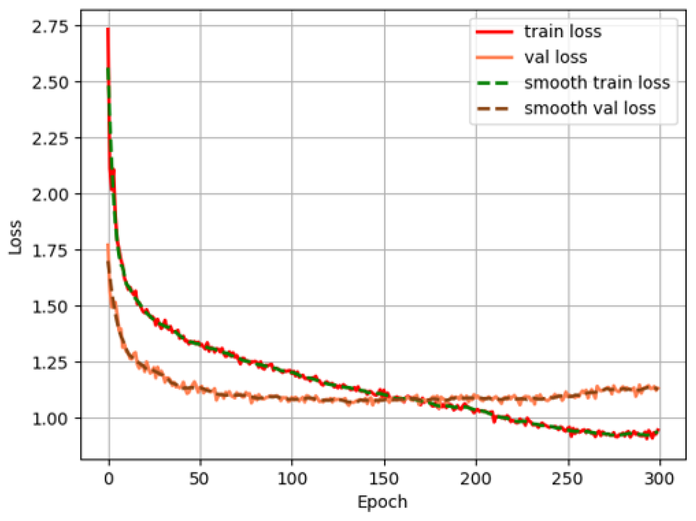
Meanwhile, for different IoU loss functions, the YOLOX model cannot converge accurately due to the symmetry of the Cartesian coordinate system, which makes the localization accuracy insufficient. In this study, the loss function of LogPolar IoU based on the Log Polar coordinate system is proposed to improve the training of the YOLOX model. Experimental evaluation is performed on a self-built dataset. The experimental results show that the LogPolar IoU-based loss function, compared with the native YOLOX loss function, improves the three models, YOLOX-tiny, YOLOX-s, and YOLOX-m, by $0.17\%$, $0.19\%$, and $0.51\%$, respectively, under the $mA{P}_{50}$ rubric. Meanwhile, the three models improve by $3.36\%$, $3.59\%$, and $2.38\%$ under the $mA{P}_{75}$ criterion, respectively, and the localization accuracy of the models based on LogPolar IoU loss function is higher than that of the models based on other versions of IoU loss function.

According to the above experimental results and conclusions, the screw localization method based on “Activate Screw Detection” proposed in this work has certain effectiveness. In addition, there are still some problems in the whole experimental process. For example, the accuracy of plane fitting depends on the accuracy of the depth image, and the accuracy of the current depth camera is not enough. The self-built dataset contains fewer kinds of screws. In future work, we will improve the robotic arm with a higher precision camera, and we will continue to expand the types and numbers of screws in the screw detection dataset to increase the generalization and robustness of the localization model. At the same time, the robotic arm used in this study has its own limitations of not being able to move. The size of the EVB is too large for the arm span of the robotic arm to cover. Therefore, in order to achieve screw detection of the whole EVB, another way out needs to be found. In future work, we will consider placing the robotic arm on a mobile cart and using the program to achieve real-time control of the cart to enable movement of the robotic arm as a way to compensate for the arm span of the robotic arm.