Article

Zero-Field Splitting in Hexacoordinate Co(II) Complexes

Department of Chemistry, Faculty of Natural Sciences, University of SS Cyril and Methodius, 91701 Trnava, Slovakia
*
Author to whom correspondence should be addressed.
Magnetochemistry 2023, 9(4), 100; https://doi.org/10.3390/magnetochemistry9040100
Submission received: 20 February 2023 / Revised: 22 March 2023 / Accepted: 3 April 2023 / Published: 4 April 2023
(This article belongs to the Section Molecular Magnetism)

Abstract

:
A collection of 24 hexacoordinate Co(II) complexes was investigated by ab initio CASSCF + NEVPT2 + SOC calculations. In addition to the energies of spin–orbit multiplets (Kramers doublets, KD) their composition of the spins is also analyzed, along with the projection norm to the effective Hamiltonian. The latter served as the evaluation of the axial and rhombic zero-field splitting parameters and the g-tensor components. The fulfilment of spin-Hamiltonian (SH) formalism was assessed by critical indicators: the projection norm for the first Kramers doublet N(KD1) > 0.7, the lowest g-tensor component g1 > 1.9, the composition of KDs from the spin states |±1/2> and |±3/2> with the dominating percentage p > 70%, and the first transition energy at the NEVPT2 level 4Δ1. Just the latter quantity causes a possible divergence of the second-order perturbation theory and a failure of the spin Hamiltonian. The data set was enriched by the structural axiality Dstr and rhombicity Estr, respectively, evaluated from the metal–ligand distances Co-O, Co-N and Co-Cl corrected to the mean values. The magnetic data (temperature dependence of the molar magnetic susceptibility, and the field dependence of the magnetization per formula unit) were fitted simultaneously, either to the Griffith–Figgis model working with 12 spin–orbit kets, or the SH-zero field splitting model that utilizes only four (fictitious) spin functions. The calculated data were analyzed using statistical methods such as Cluster Analysis and the Principal Component Analysis.

1. Introduction

Zero-field splitting (zfs) is a phenomenon of existence of fine-structure energy levels that are further split only owing to the external magnetic field. In order to avoid confusions, one has to distinguish between the experimentally verified zfs as existing energy gap(s) and the tools used for the description of zfs based upon theoretical assumptions and approximate methods. ZFS is also a source of the magnetic anisotropy reflected in the different evolution of the magnetization components, such as the easy axis or easy plane. It is generally accepted that the magnetic anisotropy of the easy axis is the crucial factor that prevents the fast magnetic relaxation via the Orbach mechanism, and secures a slow magnetic relaxation as a prerequisite of the single molecule/ion magnetism [1,2].
ZFS can be experimentally determined by various techniques, such as (i) magnetometry, (ii) susceptometry, (iii) electron paramagnetic resonance and its variants (high-field/high-frequency electron magnetic resonance), (iv) far-infrared spectroscopy and its variants in the magnetic field (FIRMS, FDMRS), (v) magnetic circular dichroism, (vi) low-temperature calorimetry, and (vii) inelastic neutron scattering [3,4,5,6,7,8,9,10,11,12,13].
ZFS can be treated as an effect of the spin–orbit interaction that splits the multielectron terms—the energy states referring to an antisymmetric wave function that accounts for the interelectron repulsion (configuration interaction) and the effects of the ligands on the central atom. The active space of kets relevant to the central atom is given by all members of the electron configuration dn that equals 10 n = 10 9 1 2 n : 10 for d1 and d9, 45 for d2 and d8, 120 for d3 and d7, 216 for d4 and d6, and 252 for d5 configurations. Working in such a space requires computer-aided efforts that, on the other hand, reduce transparency. However, the contemporary software based upon CASSCF + NEVPT2 + SOC calculations represents a useful tool in determining the spin–orbit multiplets using the fine-structure energy levels and the energy differences among them [14,15,16]. Alternate routes represent the ab initio Ligand Field Theory and the Generalized Crystal Field Theory [17,18,19].
The most common approximate concept utilized for the description of the zfs is the spin-Hamiltonian (SH) theory. This is a drastic simplification based upon reduction of the active space of kets to only a few spin functions |S, MS>: 2 to 6 kets for d1 to d9 electron configurations. For instance, for the d7 configuration, the complete (active) space consists of 120 spin–orbit kets labelled as |(νLS), J, MJ> or |Γ′,γ′,a′>, but the SH formalism works only with four spin kets |S, MS> = |3/2, ±1/2> and |3/2, ±3/2>.
The basic assumption of the SH formalism is that the effect of the spin–orbit coupling can be treated as a small perturbation. Then, the second-order perturbation theory for non-degenerate ground multielectron term offers an explicit formula for the Λ-tensor, which serves for the calculation of the spin–spin interaction D-tensor, the magnetogyric-ratio g-tensor, the temperature-independent susceptibility X-tensor, and eventually the hyperfine interaction A-tensor [20,21]. This assumption is fulfilled when the expression H = 0 H ^ so K / ( E 0 E K ) is not too large, provided by a large enough denominator as the energy gap between the ground term |0> and excited terms |K>. As an effect of small perturbation, the content of the original spin functions in the multiplets is high; in other words, SOC does not mix the spin states significantly. We will see later that this requirement alone often fails. Within the SH formalism, the energy gaps between spin–orbit multiplets are expressed in terms of the axial and rhombic zero-field splitting parameters. Notably, these D and E parameters are not observables introduced as eigenvalues of a quantum-mechanical operator. They serve as descriptive parameters and thus they should be handled with care.
The core of this review article is to show the limitations of the spin-Hamiltonian approach in treating the zero-field splitting for the difficult cases of hexacoordinate Co(II) and analogous Fe(I) and Ni(III) complexes.

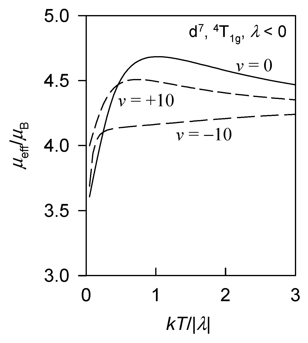
2. Theoretical Analysis

Multielectron terms in atoms are labelled by the angular momentum quantum numbers as |dn: ν, L, ML, S, MS>, where ν is the seniority number for repeated terms. On passage to the molecular systems belonging to a point group of symmetry G, the orbital part spans an irreducible representation Γ, its eventual component γ, and the branching index a, i.e., |Γ, γ, a; S, MS>; the spin part stays untouched. It is assumed that the effects of the configuration interaction are covered by the operator of the interelectron repulsion. For the irreducible representations (IRs) of the electron terms, the Mulliken notation is used, as appearing in the standard character tables of the point groups; this contains A, B, E, and T labels, with some subscripts identifying symmetry details. These definitions are compiled in Table 1.
The spin–orbit coupling in atoms causes a splitting of the atomic terms into a set of atomic multiplets; these are characterized by the total angular momentum quantum numbers |(νLS), J, MJ>. In molecules, the spin–orbit multiplets (crystal-field multiplets) are labelled according to IRs Γ′, their components γ′ and branching index a′ within the double point group G′: |Γ′, γ′, a′> [22]. Here, the Bethe notation (Γ1 to Γ8) is applied as found in character tables of the double point groups [23,24]. For Kramers systems (possessing the half-integral spin S = 1/2, 3/2, 5/2, 7/2), belonging to double groups with an order less than cubic, all IRs are doubly degenerate Γi(2); for the cubic groups, a four-fold degenerate IR also exists: Γ8(4).
The spin–orbit multiplets can be considered as observables since they are eigenvalues/eigenvectors of the operator H ^ = H ^ ee + H ^ cf + H ^ so . In the variation method, they result from the diagonalization of the interaction matrix H I J = I H ^ J where the matrix elements need to be evaluated in an appropriate basis set. The simplest approach utilizes the atomic terms as a basis set for the calculations of multiplets; other bases can be considered as a result of the unitary transformation and thus the final eigenvalues stay invariant.
Let us focus on the d7 systems exemplified by the hexacoordinate Co(II) complexes. On symmetry descent from the octahedral geometry, the orbitally triply degenerate ground term is split 4T1g4Eg   4A2g (D4h), and the excited term as 4T2g4B2g   4Eg; the orbitally non-degenerate term transforms as 4A2g4B1g. On further symmetry descent to the D2h (isomorphous with C2v), the additional splitting yields 4Eg (D4h) → 4B3g   4B2g, whereas the non-degenerate term transforms as 4A2g4B1g. The corresponding irreducible representations for spin–orbit multiplets, depending upon the respective double point group, are shown in Figure 1, Figure 2 and Figure 3.
There are several important consequences of the ground and the first excited electronic terms on the SH theory. When the ground multielectron term is orbitally degenerate (T1g or Eg), the SH formalism cannot be applied. This is a frequent mistake: sometimes the D and E values are reported; however, they are undefined when the ground state is Eg. Note that the ground electron term for the Co(II) complexes in the geometry of an elongated tetragonal bipyramid is 4Eg (the above case) and the set of the spin–orbit multiplets is labelled as Γ6, Γ6, Γ7, and Γ7. The differences among these Kramers doubles, abbr. as δ1,2, δ3,4, δ5,6, and δ7,8, cannot be expressed with the help of D- and E-parameters. The splitting between the ground term 4Eg and the first excited 4A2g is denoted as Δax, and for axial elongation it is negative. Then, the asymmetry parameter ν = Δax/λ is positive, since λ = −ξ/2S < 0 for d7 systems.
On further symmetry descent, such as D4h → D2h → C2v, the daughter terms B3g and B2g stay quasi-degenerate. Formally, the spin Hamiltonian can be applied in such a case. However, when the energy denominator in 1/(E0EK) is small, the second-order perturbation theory can suffer divergence, which manifests itself in overestimated D values and also in high asymmetry of the g-tensor components, sometimes unacceptable gi < 2.
In the opposite distortion to the compressed tetragonal bipyramid, the ground electronic term 4A2g (D4h) produces two Kramers doublets (KDs) separated by δ3,4. In this case, the crystal-field splitting parameter is positive, Δax > 0, and then the asymmetry parameter ν < 0. Now the spin Hamiltonian can be applied, assuming that Δax is not too small (when the quasi degeneracy again occurs).
The impact of the lowest terms on the magnetic properties can be visualized by plotting the effective magnetic moment against the (reduced) temperature as displayed in Figure 4. The Griffith–Figgis theory working in the space of 12 spin–orbit kets |L = 1, ML, S = 3/2, MS> allows a comparison of three cases [25]. (i) The case of a perfect octahedron (rather hypothetical due to the Jahn–Teller effect), with the ground term 4T1g for which ν = 0, displays a round maximum at the μeff vs. kT/|λ| curve. (ii) With ν > 10 (the case of an elongated bipyramid), the maximum is much reduced and the high-temperature tail almost disappears for very negative Δax; then, the effect of the low-lying excited state 4A2g is filtered off and the magnetic properties are dominated only by the eight members (4 KDs) originating in the 4Eg term. (iii) For ν < 10, the ground term is orbitally non-degenerate 4A2g and the μeff curve falls down at low temperature due to a depopulation of δ3,4 vs. the ground multiplet δ1,2. The high-temperature tail is represented by a straight line, reflecting some temperature-independent paramagnetism. The situation is well described by the SH formalism when Δax is not too small.

3. Methods and Modelling

3.1. Spin Hamiltonian

Let us recapitulate the key formulae of the spin Hamiltonian appropriate to the zero-field splitting. The spin Hamiltonian contains the axial D (rhombic E) zfs parameters
H ^ zfs = D ( S ^ z 2 S 2 / 3 ) 2 + E ( S ^ x 2 S ^ y 2 ) 2
and it is enriched by the Zeeman term
H ^ k l Z = μ B B 1 ( g x S ^ x sin ϑ k cos φ l + g y S ^ y sin ϑ k sin φ l + g z S ^ z cos ϑ k )
that depends on the polar angles { ϑ k , φ l } distributed uniformly over a sphere in order to mimic a powder average correctly. There are also higher-order zfs parameters expressed with the help of the Stevens operators [21]. Depending upon the situation, a reduced set of parameters is often utilized (D, gz, gx). Additionally, only the Cartesian components are often considered: x{π/2, 0}, y(π/2, π/2}, z{0, 0}. The diagonalization of the Hamiltonian matrix I H ^ zfs + H ^ k l Z ( B m ) J yields energy levels (two KDs for d7 systems) εkl(Bm) that depend upon discrete (at least three) values of the magnetic field. They enter the partition function Zkl(Bm, T) from which the magnetization Mkl(B, T) and magnetic susceptibility χkl(B, T) are evaluated via the first and second (numerical) derivatives with respect to the magnetic field. In addition to this universal method, there are also some simpler procedures; for instance, based upon the van Vleck equation for magnetic susceptibility. The powder average is a simple arithmetic average of the grid-dependent Mkl and χkl.
Technically, it is too ambitious to obtain reliable values of the E-parameter from the magnetic data taken above 2 K (usual range). Therefore, E as a rule is neglected. Then, the grids of the magnetic field can be limited to only a few points (e.g., 11) distributed uniformly over the half of the meridian with φ = 0 .
The magnetic anisotropy can be visualized in the 2D graphs as the separate curves Mz(B) and Mxy(B). More informative are 3D graphs, as shown in Figure 5, where the value of D > 0 leads to the easy plane and D < 0 to easy-axis magnetism.
The experimental set of DC magnetic data (temperature dependence of the molar magnetic susceptibility χ at B0 < 0.5 T, and field dependence of the magnetization per formula unit M1 at T0 < 5 K) has been fitted simultaneously by minimizing the error functional F(χ, M) → min. Several forms of the error functional have been applied; for instance, F = w 1 E ( χ ) + ( 1 w 1 ) E ( M ) , F = E ( χ ) × E ( M ) , and F = w 1 C ( χ ) + ( 1 w 1 ) C ( M ) , where the relative error E(P) and the “city-block” factor C(P) for individual observable P = χ or M are
E ( P ) = 1 N i N P i obs P i calc P i obs
C ( P ) = 1 N i N P i obs P i calc i N P i obs
In order to balance the dominating low-temperature susceptibility data against the high-temperature tail, the product P i = χ i T i or the effective magnetic moment P i = μ ( eff ) i were also used.

3.2. Griffith–Figgis Model

The GF model is based upon the Hamiltonian working in the space of twelve spin–orbit kets |L = 1, ML, S, MS> [25,26].
H ^ GF = ( λ sf A κ ) ( L p S ) 2 spin orbit   coupling + μ B B ( g e S + g L L p ) 1 spin   and   orbital   Zeeman   terms + Δ ax ( L ^ z 2 L 2 / 3 ) 2 axial   distortion + Δ rh ( L ^ x 2 L ^ x 2 ) 2 rhombic   distortion
where —spin–orbit splitting parameter modified by the Figgis CI factor A (3/2 for the weak crystal field), Δaxrh)—axial (rhombic) crystal-field splitting energy, gL = — effective orbital magnetogyric factor (negative owing to the T-p isomorphism), κ—orbital reduction factor accounting to some degree of covalency. This formula has been extended by considering the asymmetry of the Zeeman term
H ^ k l GF = A κ λ ( L p S ) 2 + [ Δ ax ( L ^ p , z 2 L p 2 / 3 ) + Δ rh ( L ^ p , x 2 L ^ p , y 2 ) ] 2 + μ B B g e ( cos ϑ k S ^ z + sin ϑ k cos φ l S ^ x + sin ϑ k sin φ l S ^ y ) 1 μ B B ( A κ z cos ϑ k L ^ p , z + A κ x sin ϑ k cos φ l L ^ p , x + A κ y sin ϑ k sin φ l L ^ p , y ) 1
where k, l define positions of the grids distributed uniformly over the polar angles { ϑ k , φ l } . In practice, k = 11 distributed along half of the meridian secures the correct powder average for the sample with an axial character. Formally, the above Hamiltonian is isomorphous to the exchange-coupled dimer, possessing the axial zero-field splitting adapted for the powder average. The energy levels obtained by the diagonalization are treated as above. This form allows a reproduction not only of the magnetic susceptibility but also the field dependence of magnetization.
The magnetic anisotropy for either Δax < 0 (easy axis) or Δax > 0 (easy plane) is essentially the same as obtained by the SH-zfs model. However, the key parameter has a completely different physical origin: in the SH-zfs model, it is the anisotropy of the fictitious spin angular momentum [ D ( S ^ z 2 S 2 / 3 ) + E ( S ^ x 2 S ^ y 2 ) ] ; in the GF model, it is the anisotropy of the orbital angular momentum [ Δ ax ( L ^ p , z 2 L p 2 / 3 ) + Δ rh ( L ^ p , x 2 L ^ p , y 2 ) ] . It can be concluded that the negative axial crystal-field splitting parameter causes the easy-axis magnetization (Figure 6).
The general procedure for evaluating the magnetic susceptibility and magnetization has been employed in order to model the temperature dependence of the effective magnetic moment and the field dependence of the magnetization for realistic parameters of the FG model relevant to Co(II) complexes (Figure 7). With Δax = ±500 cm−1, the susceptibility and magnetization curves are almost the same; some differences are seen at the effective magnetic moment. For Δax = ±1000 cm−1, the differences in the magnetization become visible; the μeff for Δax = +1000 cm−1 rises according to the straight line, which reflects the presence of the excited state manifesting itself in the temperature-independent paramagnetism. For Δax = ±3000 cm−1, the differences are substantial in magnetization, susceptibility, and effective magnetic moment. For Δax = +3000 cm−1, the effect of the excited state is filtered off and the system behaves like a typical zfs system.

3.3. Ab Initio Calculations

The only input for this kind of first-principle calculations is the molecular geometry (atomic coordinates) and the associated basis set. As the basis set, the Gaussian type functions are exclusively used with large enough angular momentum (for example, f- and g-functions for d-orbitals).
In the CASSCF (Complete Active Space Self Consistent Field) method, which is beyond the Hartree–Fock approximation, the coefficients of the linear combination of atomic orbitals (LCAO MO) and the coefficients of the configuration interaction (CI) are evaluated by the variation method. In this version of the multi-configuration method, the electrons in the active space (N, M) have variable occupations unlike those in the inactive space [27]. For transition metal complexes, the complete active space contains N d-electrons in M d-orbitals (10 spinorbitals). For a given CAS, the average energy of all states is minimized, whereas each state is weighted equally (SA-CASSCF). This version of the multi-configuration method accounts partly for the correlation energy (static correlation).
Dynamic electron correlation energy is calculated from excited configuration state functions (CSF) in which electrons are excited into empty orbitals. These CSF Φ ˜ K are used in a linear combination [28,29,30].
Ψ ˜ I = K CAS C K I Φ K + K CAS T K I Φ ˜ K
where the expansion coefficients (C and T) can be determined by application of the perturbation theory, such as second-order N-electron valence perturbation theory (NEVPT2). This method provides a second-order correction Δ E I PT 2 of the total CAS energy for each state. It is a good reference for the interpretation of excitation energies in the electronic d-d spectra.
Magnetic parameters are calculated through the quasi-degenerate perturbation theory, within which the spin–orbit coupling (SOC) operator is diagonalized over the manifold of all CAS states corrected by the NEVPT2 [31]
H I J QDPT = δ I J E I , CAS + Δ E I PT 2 + Ψ I , CAS S M H ^ SOC + Ψ J , CAS S M
The SOC operator has the Breit–Pauli form in which the spin–orbit mean-field (SOMF) approximation is used [32]
H ^ SOC SOMF = i z ^ i SOMF s ^ i
where z ^ i SOMF is an appropriately defined effective one-electron operator.
Application of the partitioning technique and/or quasi-degenerate perturbation theory yields the matrix elements of the effective Hamiltonian spanned by the spin manifold of the orbitally non-degenerate ground electronic state as follows
H M M eff = E 0 δ M M + Ψ 0 S M H ^ 1 Ψ 0 S M I S M Δ I 1 Ψ 0 S M H ^ 1 Ψ I S M Ψ I S M H ^ 1 Ψ 0 S M
with the denominator defined by excitation energies Δ I 1 = ( E I E 0 ) 1 . Then, the D-tensor and g-tensor components arising from the spin–orbit coupling are obtained using closed formulae.
An alternate way of calculating magnetic parameters (used here) is provided by the effective Hamiltonian theory [33,34]. This method is based on the construction of a model Hamiltonian which is projected into the complete space of the CAS Hamiltonian H ^ rel in the sense of des Cloizeaux definition of the effective Hamiltonian
H ^ C eff = k Ψ ˜ k C E k Ψ ˜ k C
Here, the effective Hamiltonian reproduces the energy levels of the CAS Hamiltonian Ek and the wavefunctions of the states projected to the model space Ψ ˜ k . Using a singular value decomposition procedure, the elements of D- and g-tensor are extracted [35]. In case of the low norm of the projections (N << 1), the trial model Hamiltonian is inapplicable to the given system.
All calculations were conducted using the ORCA package [14,15,36] in the experimental geometry of Co(II) complexes (neutral or charged). As a basis set, ZORA-def2-SV(P) was used for non-metal atoms, and ZORA-def2-TZVPP for the Co(II) center.

3.4. Generalized Crystal-Field Theory

This method (GCFT) works in the basis set of atomic terms characterized by the angular momentum quantum numbers I = d n : ν , L , M L , S , M S . The space covers 120 kets for a d7 system like in the CAS method. By applying the irreducible tensor algebra, the matrix elements of the interaction operators are evaluated: the interelectron repulsion H ^ ee , crystal field H ^ cf , spin–orbit coupling H ^ so , Zeeman orbital, and Zeeman spin interactions [18,19,37]. The parameters dependent upon the radial functions are expressed by the Racah B and C parameters for the interelectron repulsion, and the crystal-field poles F2(L) and F4(L) for individual ligands L, respectively. The angular parts of the matrix elements are integrated using coefficients of fractional parentage and vector coupling coefficients (3j- and 6j-symbols). The positions of ligands involve the spherical harmonic functions owing to which the matrix elements are complex. The spin–orbit interaction is characterized by the spin–orbit coupling constant ξCo. The diagonalization of the matrix J H ^ ee ( B , C ) + H ^ cf ( F 2 , F 4 ) + H ^ so ( ξ ) I yields the crystal-field multiplets K = ( d n ν L S ) ;   Γ a , γ a , a , where we used labelling of the irreducible representations (IRs) and their components {   Γ a , γ a , a } within the double point group of symmetry.
The evaluation of the spin-Hamiltonian parameters represents an approximation based upon the construction of the Λ-tensor by means of the second-order perturbation theory
Λ a b = 2 J 0 0 L ^ a J J L ^ b 0 / ( E J E 0 )
where the summation runs over all excited terms J . The Λ-tensor is used in the definition of the D-tensor D a b = λ 2 Λ a b . In the traceless form
D a b = D a b δ a b ( D x x + D y y + D z z ) / 3
the axial and rhombic zero-field splitting parameters are expressed as
D = ( D x x D y y + 2 D z z ) / 2
E = ( D x x D y y ) / 2
In the GCFT calculations, the key role plays an appropriate choice of the crystal field poles F4(L) and eventually F2(L) for individual ligands. This method is suitable for the modelling of SH parameters over a wide range of geometries and crystal-field strengths.

4. Results and Discussion

4.1. Geometry of Complexes

The complexes under study have the shape of an elongated or compressed tetragonal bipyramid with some o-rhombic component in the equatorial plane (Table 2). Distances on the trans-ordinate were averaged and further processed as follows. Assuming that the highest eccentricity lies along the z-axis, the structural distortion parameters are defined as
D str = ( d i d ¯ i ) z [ ( d i d ¯ i ) x + ( d i d ¯ i ) y ] / 2
E str = [ ( d i d ¯ i ) x ( d i d ¯ i ) y ] / 2
where d ¯ i is the mean distance for a given bond (i = N, O, Cl). These have been taken from compounds containing the [Co(NH3)6]2+, [Co(H2O)6]2+ and [CoCl6]4− complex units, giving rise to d ¯ ( Co N ) = 2.185 Å, d ¯ ( Co O ) = 2.085 Å, and d ¯ ( Co Cl ) = 2.475 Å [38]. This procedure is effective for complexes with a heterogeneous donor set with different averaged metal–ligand distances. Sometimes it is not clear which distances should be selected as axial, and which as equatorial. Hereafter, a constraint is utilized: Estr/|Dstr| < 1/3. (Analogous constraints are used for axial and rhombic zero-field splitting parameters in SH theory.) Some of the studied complexes possess the form of a pincer-type: there are severe deviations of four donor atoms from the equatorial plane due to the rigidity of the organic ligand. Therefore, the values of Dstr* need to be handled with care.
In some cases, the compound contains two crystallographic independent complex units. The ab initio calculations were performed for each of them. Some compounds contain identical or similar structural units. In the series [Co(dppmO,O)3][Co(NCS)4] (J), [Co(dppmO,O)3][CoBr4] (K) and [Co(dppmO,O)3][CoI4] (L) with the chromophores {CoO2O’2O”2}, the values of Dstr vary as −1.65, −1.45, and +2.15 pm; [Co(dppmO,O)3][CoCl4] (U) has a different symmetry of the chromophore {CoO3O’3}. The complex [Co(pydm)2](dnbz)2 (O) is analogous to [Co(pydm)2](mdnbz)2 (P), but differing in Dstr = −20.1 and −17.9 pm. Finally, [Co(bzpy)4Cl2] (F) contains two crystallographic different units with Dstr = +7.05 and −3.5 pm.

4.2. Elongated Tetragonal Bipyramid

Some hexacoordinate Co(II) complexes possess the geometry of the chromophore close to the elongated tetragonal bipyramid with eventual small o-rhombic component. Their structural parameter (axiality) is Dstr > 0. In such a case, it is expected that the temperature dependence of the effective magnetic moment passes through a round maximum (which not necessarily is visible until room temperature). The effective magnetic moment exceeds μeff > 5 μB and the magnetization per formula unit saturates close to M1 = Mmol/(NAμB) ~ 3. In some cases, the magnetic data have been refitted by a more appropriate model than published previously. Note that the magnetization data can suffer of some orientation effect in higher fields especially when the rso- or vsm-mode of detection is used in the modern SQUID apparatus. Then, the detected magnetization data could be a bit higher than calculated by the fitting procedure which equally weights the susceptibility data taken in small DC field. The free parameters also cover some temperature-independent (para)magnetism χTIM that influences the high-temperature tail of the magnetic susceptibility, and the molecular field correction zj effective at the lowest temperatures (not listed here).
The key results of the ab initio calculations and fitted magnetic data (susceptibility and magnetization) are presented in Table 2. Certain calculations were redone with respect to the published data in order to keep the same basis set. The success of the spin-Hamiltonian theory is classified as either 5—fulfilled, 4—acceptable, 3—questionable, 2—problematic, or 1—invalid. However, such a classification is rather subjective; a more objective classification is the quantitative evaluation of the spin Hamiltonian according to the score S1, introduced as follows:
S1 = N(KD1)·g1·[E(KD3) − E(KD2)]·Δ1/10,000
The set of critical parameters involves the norm of the projected state for the first Kramers doublet N(KD1), the smallest g-tensor component g1, the separation of the two subsets of KDs [E(KD3) − E(KD2)], and the first transition energy at the NEVPT2 level 4Δ1 (scaled to smaller numbers). Values of S1 > 50 refer to class 5—fulfilled; S1 < 10 span class 1—invalid. Limiting value for the fulfillment is S1 = 0.7 × 1.9 × 600 × 600/10,000 = 48. The above parameter can be extended by considering the mixing of the spin states: S2 = S1 × P/100 where P—percentage of the greater portion of spins | ± 1/2> or | ± 3/2> in the first KD (ideally p > 70).
The simplest complex containing the hexa-aqua ligands is [Co(H2O)6]2+(OHnic)2 (A). The complex cation adopts the geometry of an elongated tetragonal bipyramid with a considerable axiality and zero rhombicity, Dstr = +7.1 pm and Estr = 0. The orbitally degenerate ground term 4T1g (Oh) causes the Jahn–Teller effect, leading to the symmetry descent, and consequently to the splitting of the ground mother term. The energies of the daughter terms lie at {0, 199, 2468} cm−1, which is consistent with the ground term 4Eg and the excited 4A2g2 = 2468 cm−1). Small splitting of the ground term {0, 199} cm−1 is caused by “innocent” hydrogen atoms that disturb the ideal D4h symmetry (the ground state is orbitally quasi-degenerate). As valuable results, comparable with experiments, serve the energies of Kramers doublets δ{0, 209, 526, 814} cm−1, the transitions among them can be identified, for instance, by the FAR-infrared spectra. Rather unexpected is the fact that the compositions of these KDs contain almost equal contributions from | ± 1/2> and | ± 3/2> spins. This means that the spin–orbit coupling seriously mixes the states of the different spin projections, or in other words, H ^ so cannot be considered as a small perturbation. Therefore, all “products” of the spin Hamiltonian can be false. Indeed, g1 = 1.76 << 2, D = −101 cm−1 are artefacts and this conclusion is also supported by the small norm of the projected state N(KD1) = 0.61 << 1. The attempts to fit the magnetic data with the GF model were successful: the round maximum at the effective magnetic moment was perfectly reproduced with λeff = Aκλ = −188 cm−1, gL = −1.10, and Δax = −112 cm−1.
The complex [CoIICoIII(L1H2)2(H2O)(ac)]·(H2O)3 (B) contains the homogeneous donor set {CoO4O’2} with averaged distances Co-Oeq = 2.061 and Co-Oax = 2.150 Å owing to which Dstr = +8.9 pm. The energies of KDs are δ{(0, 220), (736, 1006)} cm−1, and they are better separated owing to higher Δ2 = 1516 cm−1. The secondary splitting of 4Eg term is Δ1 = 444 cm−1 so that the orbital degeneracy is partly removed. However, there are critical indicators warning that the spin-Hamiltonian theory is questionable in the present case: N(KD1) = 0.71, g1 = 1.84, and severe mixing of the spin states with the principal contribution < 0.7; D = −101 cm−1. GF Hamiltonian was used in fitting the magnetic data with Δax < 0 resulting in λeff = −198 cm−1, gLz = −1.64, gLx = −1.11, and Δax = −774 cm−1.
The complex trans-[Co(bz)2(H2O)2(nca)2] (C), after the corrections to the heterogeneous donor set {CoO2Ow2N2}, possesses Dstr = +7.75; its room-temperature effective magnetic moment reaches μeff ~ 5 μB and the magnetization saturates close to M1 ~ 3. These features are typical for systems with the ground electronic term 4Eg for which the spin-Hamiltonian formalism could fail. The energies of KDs are not well separated into two subsets of KDs δ{0, 256, 525, 850} cm−1. The critical indicators are: N(KD1) = 0.58, g1 = 1.51, 4Δ1 = 117 cm−1 (almost degenerate ground state), and a boundary mixing of the spin states; D = −113 cm−1 could be an artefact. The fitting of magnetic data based upon the GF Hamiltonian gave λeff = −172 cm−1, gLz = −2.06, gLx = −1.50, and Δax = −739 cm−1.
In the complex [Co(acac)2(H2O)2] (D) with the chromophore {CoO4Ow2}, the longest distance is Co-Ow = 2.157 Å gave Dstr = +12.0 pm. The energies of KDs are δ{(0, 155), (915, 1153)} cm−1 and they form two well separated sub-sets. Additionally, the energy of the first electronic transition 4Δ1 = 763 cm−1 suggests that the ground state is well separated from the excited counterpart. Therefore, the spin-Hamiltonian formalism could work, which is also supported by the critical indicators N(KD1) = 0.81 and g1 = 1.943, yielding the score S1 = 91. The calculated D = +73 cm−1 and E/D = 0.23 yield an estimate of the energy gap G3,4 = 2(D2 + 3E2)1/2 = 2|D|[1 + 3(E/D)2]1/2 = 155 cm−1 that equals the energy of the KD2 δ3,4 = 155 cm−1. The calculated magnetic susceptibility passes through the experimental points and the magnetization per formula unit amounts to Mmol/(NAμB) = 2.35 at B = 7.0 T.
The complex [CoL22Cl2] with the {CoO2N2Cl2} chromophore (E), after correction to the heterogeneity of the donor set, displays Dstr = +9.45 pm with large rhombicity Estr = 2.65 pm (Estr/Dstr = 0.28) close to the critical value of 0.33 when the sign of the Dstr is uncertain. The alternate structural parameters are Dstr = −8.7, Estr = 3.4 pm, and Estr/Dstr = 0.39. The ab initio calculations confirm that the SH theory for this system is appropriate since N(KD1) = 0.91, g1 = 2.03, 4Δ1 = 1217 cm−1, and a weak mixing of spin states exists: D = +43 cm−1. The estimated energy gap G3,4 =2(D2 + 3E2)1/2 = 94 cm−1 matches perfectly the energy of the KD2 δ3,4 = 94 cm−1. The magnetic data were fitted with the SH-zfs model using D = 75, °E = 4.8 cm−1, and g{2.51, 2.36, 2.0}.
The compound [Co(bzpy)4Cl2] contains two crystallographic independent molecular complexes with different axiality Dstr = +7.05 and −3.5 pm, respectively. The unit Fa possesses two well-separated subsets of KDs δ{(0, 179), (633, 911)} cm−1. The first transition energy 4Δ1 = 448 cm−1 indicates that the orbital degeneracy is partly removed. Critical indicators classify the SH as acceptable and calculated D = 88 cm−1 as reasonable. The unit Fb displays different properties: not separated groups of KDs δ{0, 252, 455, 787} cm−1, N(KD1) = 0.49, orbital degeneracy 4Δ1 = 130 cm−1, and subnormal g1 = 1.60 that approves classification of SH as invalid. Though the ab initio calculations were performed for individual units separately, the magnetic data reflect some average of their response. The GF model gave λeff = −175 cm−1, gLz = −1.02, gLx = −1.28, and Δax = −424 cm−1, whereas the SH-zfs model yields D = +106 cm−1 and gx = 2.53.

4.3. Nearly Octahedral Systems

Since the distance-corrected values d ¯ (Co-O) and d ¯ (Co-N) can vary [46], complexes with small negative or small positive Dstr were included in this group. The results of ab initio calculations and magnetic data fitted either with the GF or SH-zfs model are presented in Table 3.
The compound [Co(hfac)2(etpy)2] contains two independent crystallographic units, and thus ab initio calculations were performed for both of them. The unit Ga shows four KDs at δ{0, 237, 461, 804} cm−1 with a serious mixing of spin states. The critical indicators show that the SH theory is invalid: N(KD1) = 0.50; g1 = 1.66 (subnormal), 4Δ1 = 109 cm−1 (quasi degeneracy). The unit Gb possesses a better separation of the two subgroups of KDs δ{(0, 196), (568, 873)} cm−1 owing to increased transition energy 4Δ1 = 359 cm−1. The critical indicators are N(KD1) = 0.64; g1 = 1.93 (SH is still problematic). Both complexes have small negative Dstr = −2.00 and −2.45 pm, which prefer the application of the GF model for the magnetic data fitting with λeff = −159 cm−1, gLz = −1.96, gLx = −1.79, and Δax = −771 cm−1.
An analogous complex [Co(hfac)2(bzpyCl)2] (H) shows Dstr = −2.45 pm with well-separated subgroups of KDs δ{(0, 188), (582, 883)} cm−1. The set of indicators is still critical: N(KD1) = 0.58; g1 = 1.95, 4Δ1 = 392 cm−1 (degeneracy is partly lifted), and the mixing of spin states is rather weak. The SH formalism is problematic; D = +91 cm−1. The GF model for the magnetic data fitting gave λeff = −170 cm−1, gLz = −1.83, gLx = −1.11, and Δax = −643 cm−1.
The molecular complex [Co(abpt)2(tcm)2] (I) displays small Dstr = −2.0 pm. All critical indicators confirm that the SH formalism is fulfilled: δ{(0, 131), (862, 1066)} cm−1, N(KD1) = 0.86; g1 = 2.04, 4Δ1 = 900 cm−1 (orbital degeneracy lifted), weak mixing of spin states. Then, the evaluated D = +50 cm−1 can be considered as a valid parameter. The composition of the ground KD1 is {20·| ± 1/2> + 79·| ± 3/2>} with dominating contributions of | ± 3/2>; for D > 0, just | ± 1/2> is expected as a dominating component of the ground multiplet Γ6. Perhaps large rhombicity E/D = 0.29 causes this feature.
Three complexes of the type [Co(dppmO,O)3][CoX4], X = NCS, Br and I possess the same cationic complex (with 154 atoms) with small axiality Dstr = −1.65, −1.45, and +2.15 pm, respectively. (The fourth member with X = Cl has a different geometry of the chromophore {CoO3O’3}.) The presence of the complex anions was not involved in calculations; however, the experimental data reflect their effect on the increased values of the effective magnetic moment and magnetization.
The complex cation in [Co(dppmO,O)3][Co(NCS)4] (J) possesses δ{(0, 211), (562, 966)} cm−1, g1 = 1.97, 4Δ1 = 445 cm−1 (degeneracy partly lifted), but a serious mixing of spin states. Therefore, it is classified as SH–problematic; D(Oh) = +105 cm−1. Note that the solid-state magnetic data were fitted assuming the presence of both nearly octahedral and nearly tetrahedral units with D(Oh) = 91, D(Td) = −5.0 cm−1.
The complex cation in [Co(dppmO,O)3][CoBr4] (K) behaves analogously to its NCS analogue: δ{(0, 211), (562, 966)} cm−1, g1 = 1.97, 4Δ1 = 445 cm−1 (degeneracy partly lifted), N(KD1) = 0.61 and a serious mixing of spin states; D(Oh) = +105 cm−1. The SH is classified as problematic and the fitting of magnetic data gave D(Oh) = +122 and D(Td) = +15 cm−1.
The complex [Co(dppmO,O)3][CoI4] (L) with δ{(0, 223), (508, 874)} cm−1 shows different critical parameters: 4Δ1 = 258 cm−1 (near degeneracy), subnormal g1 = 1.86 and again a strong mixing of spin states. The SH is classified as invalid; calculated D(Oh) = +107 cm−1 and fitted D(Oh) = +99 and D(Td) = +19 cm−1.
In summary, the ab initio calculations for nearly octahedral Co(II) complexes predicted D > 0 when the spin Hamiltonian was appropriate and matching the magnetic data fitting.

4.4. Compressed Tetragonal Bipyramid

This numerous group involves complexes with a considerable negative axiality of Dstr << 3 (Table 4). In general, the magnetic data for them can be fitted with the SH-zfs model which assumes gz = 2, gx >> 2, D >> 0. Alternatively, the GF model can also be used with Δax > 0.
The complex [Co(iz)6](fm)2 (M) with the homogeneous ligand sphere contains the {CoN6} chromophore that can be classified as a compressed tetragonal bipyramid with considerable, but negative axiality and small rhombicity: Dstr = −6.10 and Estr = 0.71 pm. The energies of the spin–orbit multiplets δ{0, 256, 450, 836} cm−1 are quite similar to the complex [Co(H2O)6](OHnic)2 (A). There is a set of critical indicators warning that the spin-Hamiltonian theory fails: N(KD1) = 0.46, 4Δ1 = 35 cm−1 (orbital degeneracy), g1 = 1.30, g2 = 1.83 (subnormal values), and severe mixing of the spin states; D = +124 cm−1. Nevertheless, the magnetic data were fitted with the SH-zfs model with parameters D = +69 cm−1 and gx = 2.75.
The compound [Co(bzpy)4(NCS)2] contains two crystallographic independent molecular complexes with Dstr = −11.75 and −11.05 pm, respectively. The electronic properties of them are similar: two subgroups of KDs δ{(0, 187), (646, 965)} cm−1, 4Δ1 = 473 cm−1 and g1 = 1.93. Therefore, the SH is classified as questionable; D = +89 cm−1 for Na (and similar for Nb). The magnetic data fitting using the SH model gave D = +95 cm−1 and gx = 2.52.
The cationic complex of [Co(pydm)2](dnbz)2 (O) contains the pincer-type ligands pydm which, owing to a rigidity, do not coordinate on the axes of the equatorial plane, so that the values of Dstr* = −20.15 pm need be considered with care. Two sub-set of KDs are well separated δ{(0, 188), (864, 1099)} cm−1 owing to increased 4Δ1 = 614 cm−1. The critical parameters indicate that the SH might be fulfilled: N(KD1) = 0.71, g1 = 1.98, weak mixing of spin states. The only disturbance is the negative value of D = −92 cm−1, since positive value is expected for the compressed tetragonal bipyramid. This point will be explained later using the GCFT calculations.
An analogous compound contains the same cationic complex [Co(pydm)2](mdnbz)2 (P) with the same pincer ligand but slightly modified counter anion; Dstr* = −17.9 pm. Again, two groups of KDs are well separated δ{(0, 145), (870, 1099)} cm−1 and the first transition energy is 4Δ1 = 708 cm−1. However, N(KD1) = 0.68 and increased mixing of the spin states cause the classification of the SH—close to fulfilled. Again, negative D = −69 cm−1 was calculated for this system. With this data, the energy gap G3,4 = 145 cm−1 matches the energy of the first excited KD, δ3,4 = 145 cm−1. The magnetic data were fitted almost perfectly using the SH-zfs model with D = −50 cm−1.
The compound [Co(pydca)(dmpy)]·0.5H2O contains two crystallographic independent units, both with negative axiality Dstr = −22.65 pm. The site Qa possesses well-separated subgroups of KDs δ{(0, 162), (813, 1046)} and 4Δ1 = 614 cm−1. The critical indicators signalize that the SH is fulfilled: N(KD1) = 0.78, g1 = 1.99; only the mixing of the spin states is stronger. The unit Qb exhibits similar characteristics with D = −97 cm−1 in comparison with D = −77 cm−1 for Qa. The fitting of the magnetic data with the SH-zfs model gave D = −89 cm−1, gz = 2.50, and gx = 2.42.
The complex [Co(ac)2(H2O)2(MeIm)2] (R) possesses Dstr = −11.9 pm and the ab initio data confirm a separation of the two subsets of KDs δ{(0, 156), (1030, 1230)} cm−1 owing to large 4Δ1 = 878 cm−1. The critical indicators show that the SH is fulfilled: N(KD1) = 0.84 and g1 = 1.91. With expectations, D = +75 cm−1 is positive for compressed tetragonal bipyramid. There is a serious mixing of spin states. The same quality of the magnetic data fits was obtained using the GF model (λeff = −217 cm−1, gLz = −1.23, gLx = −1.37, Δax = +568 cm−1) and/or the SH-zfs model (D = +82 cm−1, gx = 2.54).
The complex trans-[Co(ampyd)2Cl2] (S) possesses Dstr = −7.03 and the critical indicators warn that the SH fails: N(KD1) = 0.50, subnormal g1 = 1.43, and g2 = 1.90, very small transition energy 4Δ1 = 76.6 cm−1 which causes the two subgroups of KDs to not be separated δ{0, 262, 461, 800} cm−1. Then, the calculated D = +121 cm−1 is false and the magnetic data fitting is not satisfactory when the SH is used. The GF model gave acceptable fit with λeff = −181 cm−1, gLz = −1.5, gLx = −1.3, and Δax = +377 cm−1.

4.5. Miscellaneous Geometry

This section involves data for complexes that do not span the above three classes: the structural axiality Dstr is either undefined or oddly defined (Table 5). It shows a versatility of the magnetic behavior of hexacoordinate Co(II) complexes.
The complex [Co(dppmO,O)3][CoCl4] (T) spans the series [Co(dppmO,O)3][CoX4], but unlike the NCS, Br, and I members, it displays different geometry of the {CoO3O3′} chromophore so that axiality Dstr is not defined in this case. The critical indicators warn that the SH is not fulfilled, since g1 = 1.78, 4Δ1 = 150.6, and 4Δ2 = 150.9 cm−1, strong mixing of spin states are demonstrated, and not separated subsets of KDs δ{0, 314, 393, 926} cm−1. Therefore, the calculated D = +157 cm−1 could be false. However, the magnetic data were satisfactorily fitted with D = +77 cm−1.
The complex cis-[Co(phen)2(dca)2] exists as two polymorphs (Ua, Ub) and again does not fulfil the definition of axiality Dstr. According to the critical indicators for Ua, the SH is classified as invalid: N(KD1) = 0.54, g1 = 1.49, very low transition energy 4Δ1 = 110 cm−1, and the two subsets of KDs not separated δ{0, 243, 495, 838} cm−1. The calculated value of D = +108 cm−1 seems be overestimated. The magnetic data were fitted with D = 91 cm−1 and gx = 2.66; however, the fit was not satisfactory for the magnetization data. For the polymorph Ub, the situation was completely different with a high score of S1 = 51 (mainly due to the high first transition energy 4Δ1 = 618 cm−1) that allows a classification of the SH as fulfilled. At the same time, both the susceptibility and magnetization data were fitted excellently using D = 85 cm−1 and gx = 2.60.
The complex cation in [Co(pypz)2](tcm)2 (V) possesses the considerable axiality Dstr = −8.2, Estr = 0. However, the deviations of four N-donor atoms from the equatorial plane are not negligible owing to the rigid geometry of the pincer-type ligand. The energies of KDs are split into two well-separated subsets δ{(0, 159), (717, 1003)} cm−1, owing to the removal of the orbital degeneracy, 4Δ1 = 571 cm−1. The critical indicators confirm that the SH is fulfilled: N(KD1) = 0.74, g1 = 1.99, weak mixing of spin states; the value of D = +72 cm−1 is fully acceptable. However, the calculations were performed for a free complex cation abstracting from the environment. The environment alone plays a critical role, since the tcm ligands link several cationic units into a complex network which shows features of the exchange interaction of a ferromagnetic nature. The magnetic susceptibility passes through a maximum that is typical for tetragonal systems with positive axiality, and at the same time the magnetization per formula unit exceeds a value of M1 > 3. The magnetic data cannot be fitted by a reliable set of parameters using both GF and SH-zfs models for a single magnetic center.
The complex [μ-(dca)Co(pypz)(H2O)] dca (W) has structure of a 1D chain decorated by free dca ions. The ab initio calculations were not performed; the magnetic data were fitted with the GF model.

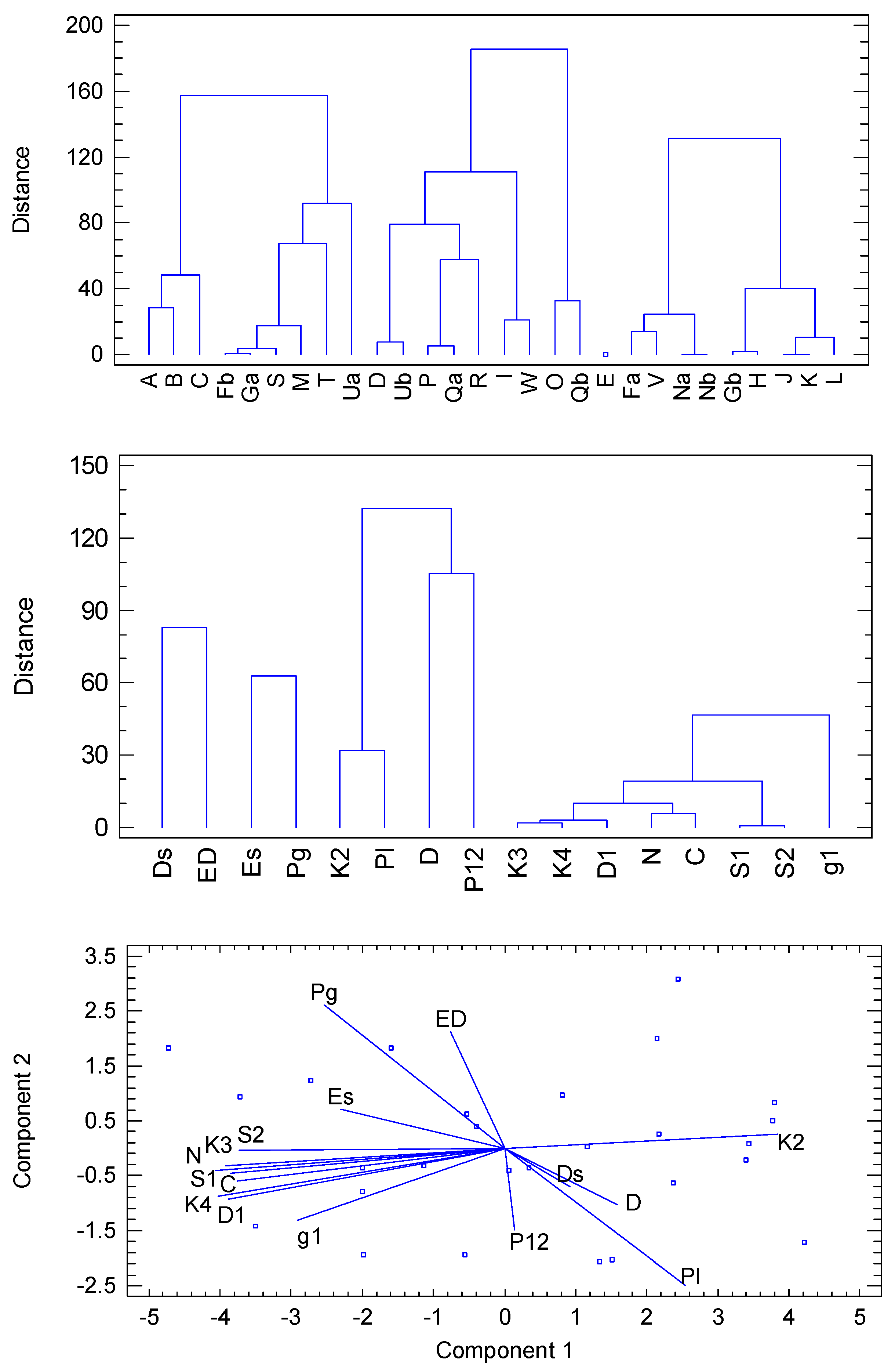
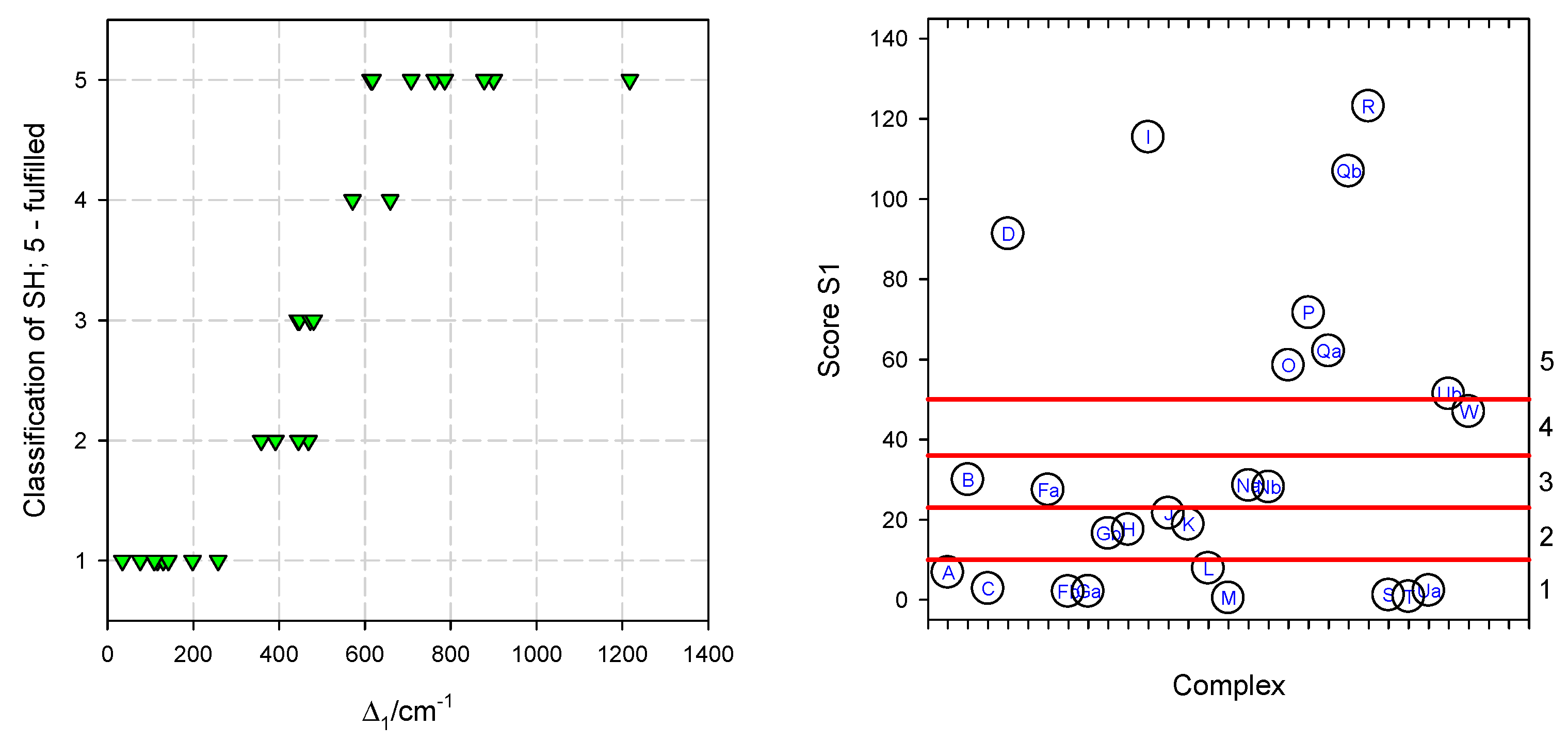
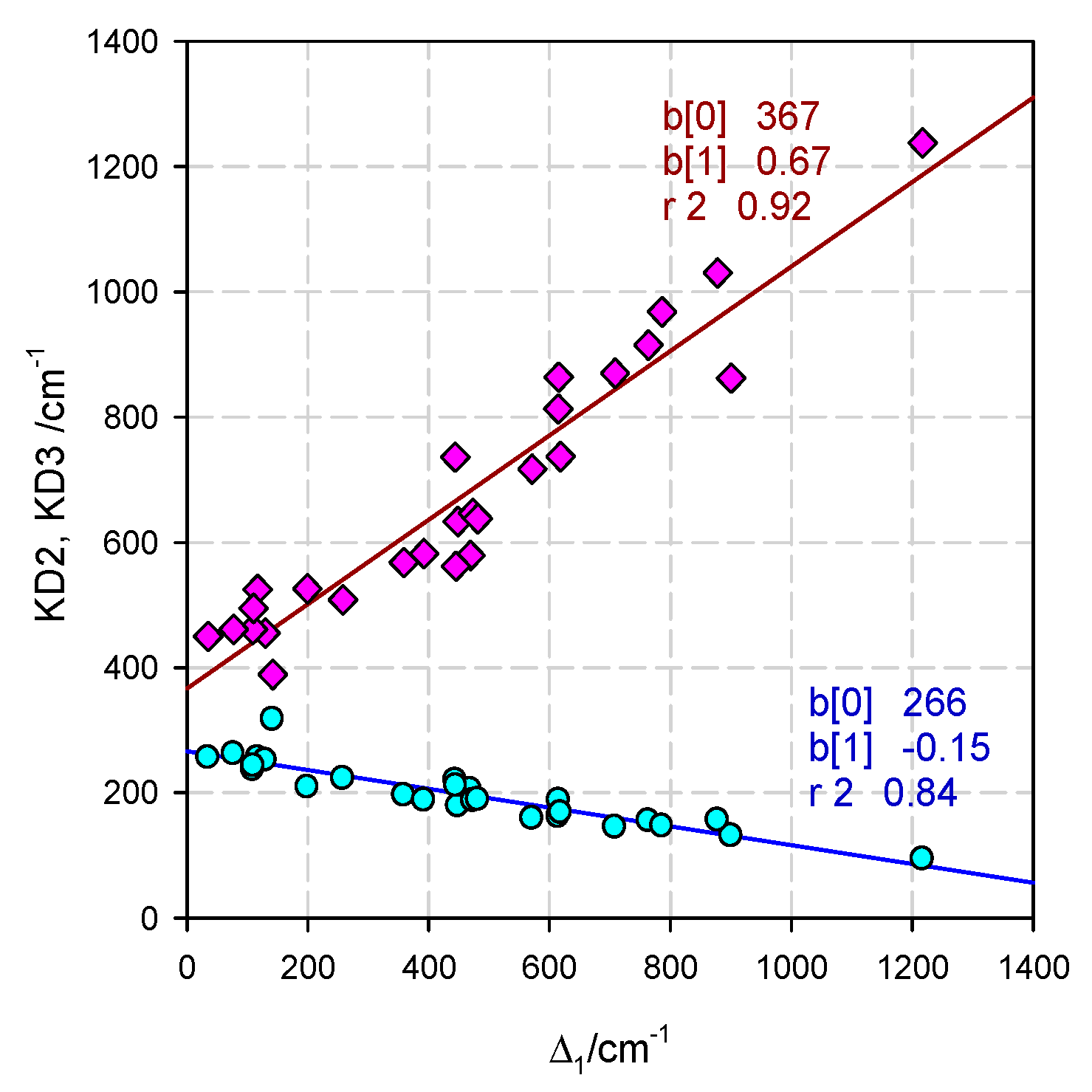
5. Statistical Analysis

The calculated ab initio data were used to form a worksheet for modern statistical analysis [60]. The Cluster Analysis divides the observables according to the “distance” into four or five groups; for codes, see Figure 8.
Complementary information brings the biplot of the Principal Component Analysis: (i) with decreasing D1, the energy of K2 increases and simultaneously the energies of K3 and K4 decrease; (ii) at the same time, the critical indicators g1 and N decrease, thus showing a failure of the spin-Hamiltonian formalism; (iii) D correlates with Ds; and (iv) C anticorrelates with D (with increasing calculated D, the classification factor C decreases from 5 to 1).
The classification score of the spin Hamiltonian (between 1 to 5) correlates with the first transition energy 4Δ1 (Figure 9). For Δ1 < 300 cm−1, the SH data are barely reliable (class 1) because of the quasi-degeneracy. For Δ1 > 600 cm−1, the SH data are highly reliable (class 4 or 5). A numerical correlation including the correlation coefficient is presented in Figure 10.
The sign of the axial zero-field splitting parameter D attracts great attention, mainly in the light of the D-U paradigm, according to which the barrier to spin reversal U for the Orbach process of slow magnetic relaxation fulfills the relationship U = |D|(S2 − 1/4) for Kramers systems [1]. A deeper analysis of experimental data shows: (i) slow magnetic relaxation exists also in systems with D—positive, negligible, or in systems where D is undefined (S = 1/2); (ii) quantitatively, the above paradigm is not true, at least for the hexacoordinate Co(II) complexes. In the cases of hexacoordinate Co(II) complexes when the SH is fulfilled (D4h, D2h symmetry of the chromophore), D > 0 generally holds true. Ab initio calculations can indicate some D < 0; however, in the cases when HS fails (Dstr >> 0).
There is an exception for complexes containing the pincer-type ligands when the donor set occupies sites outside the axes of the equatorial plane. This point has already been modelled by using GCFT calculations, as depicted in Figure 11 [51].
The GCFT allows a wide-range modelling of the energies of spin–orbit multiplets (KDs) δi,i+1 and SH parameters (D, gz, gx, χTIP) depending upon the strength of the crystal field poles F4(ax) and F4(eq); the results are presented in Figure 12. For the elongated tetragonal bipyramid, the D-values are undefined, since the ground term is orbitally degenerate 4Eg and the two lowest multiplets span the irreducible representations Γ6 and Γ6.
A majority of hexacoordinate Co(II) complexes investigated in this work were tested for a slow magnetic relaxation (SMR), and all of the tested cases confirm the presence of SMR. The existence of SMR is independent of the geometry—whether the complex belongs to the elongated or compressed tetragonal bipyramid, the nearly octahedral, or miscellaneous geometry. The contemporary state of the art is as follows (Figure 13). (i) A more careful data selection at low frequencies of the oscillating AC magnetic field reveals the second (LF) and eventually third (IF) relaxation channel in addition to the high-frequency (HF) one. These channels are strongly dependent upon the applied DC field. (ii) The low-frequency relaxation channel attenuates on heating more progressively than the HF one. (iii) The temperature ranges, in which the maximum (maxima) on the out-of-phase susceptibility is visible, are often limited to T < 6 K. (iv) The analysis of the relaxation data according to the Arrhenius-like equation τ = τ0exp(U/kBT) is appropriate only for the Orbach relaxation process. Using a few high-temperature data, the evaluation of the extrapolated relaxation time (for infinite temperature) τ0, and the barrier to spin reversal U is often possible; however, it can yield incorrect values when the slow relaxation at the highest edge of the data taking is not attenuated. The collection of {D, U, τ0} data is of little value when the relaxation proceeds according to the alternate mechanisms such as Raman, phonon bottleneck, and direct relaxation mechanisms. (v) The plot lnτ vs. lnT brings information about the temperature coefficient in the above mechanisms proceeding via eqn. τ−1 = CTm: m ~ 1 for the direct process, m ~ 2 for the phonon bottleneck process, or m = 5–9 for the Raman process. The Orbach process requires m > 9, which, as a rule, is not the case. Data in Figure 13 confirm that the HF relaxation mode at elevated temperatures proceeds via the Raman mechanism with the temperature coefficient m = 5.9; at low temperature, a reciprocating thermal behavior applies, m = −0.64 when on cooling the relaxation time decreases [61,62].
The final critical remark is addressed to the spin-Hamiltonian formalism that considers the existence of only two KDs separated by 2D. If this gap, for instance, is only G = 100 cm−1 (144 K), then the Boltzmann population of KD2 at T = 10 K is P3,4 = 2 × (5.6 × 10−7), i.e., negligible. This discriminates the Orbach relaxation mechanism and related U and τ0 as unrealistic parameters. In the light of these findings, the value of the collection of the published data on D and their relationship to U in hexacoordinate Co(II) complexes is questionable [63]. There are several original and review articles about the impact of the zero-field splitting on the DC and AC magnetic properties of hexacoordinate Co(II) complexes; some of them are accompanied by ab initio calculations; however, a deeper validity assessment of the spin-Hamiltonian formalism is missing [64,65,66,67,68,69,70].

6. Conclusions

The hexacoordinate Co(II) complexes can be classified into four groups according to their structural axiality (tetragonality) Dstr: (i) complexes with large positive values referring to the elongated tetragonal bipyramid (with some o-rhombicity); (ii) nearly octahedral complexes with small |Dstr|; (iii) complexes with large negative Dstr referring to the compressed tetragonal bipyramid; and (iv) complexes with miscellaneous geometry. The first type possesses the ground electronic terms orbitally (nearly) degenerate 4Eg (with corresponding daughter terms on symmetry lowering). The spin Hamiltonian, as a rule, fails, and thus the magnetic data need to be fitted by employing the extended Griffith–Figgis model working in the space of 12 spin–orbit kets. The GF theory is an intermediate step between the spin Hamiltonian recognizing only 4 (fictitious) spin kets and the complete active space of 120 kets generated by the d7 configuration.
The activation of the spin-Hamiltonian formalism in the first-principle calculations yields the D-parameters that could be false. Typically, D > 0 holds true for hexacoordinate Co(II) complexes with the exception of those with pincer-type ligands. The perfect fulfilment of the spin-Hamiltonian formalism is rather rare; some critical indicators allow a classification as 5—fulfilled, 4—acceptable, 3—questionable, 2—problematic, and 1—invalid. Of 24 compounds containing 28 hexacoordinate complexes studied by ab initio method, only 10 span the categories 5 and 4, and 9 the category 1. The failure of the SH manifests itself in low first transition energy° 4Δ1 < 300 cm−1, low projection norm N(KD1) < 0.7, subnormal value of the lowest g-factor g1 < 1.9, and large mixing of the spin components into multiplets with the highest portion p < 70%. In such a case, the second-order perturbation theory tends to diverge and the calculated D parameters are overestimated. The statistical methods (Cluster Analysis, Principal Component Analysis) bring information which parameters mutually correlate.
The D values obtained by fitting the magnetic data are risky to accept without deep theoretical analysis. The first energy gap given by the energy of the second Kramers doublet G = δ3,4 can be reconstructed by assuming G = 2|D|, or G = 2(D2 + 3E2)1/2. Thus, the successful fit itself is not a guarantee that the spin-Hamiltonian formalism is fulfilled for the given case. The main obstacle lies in the fact that for hexacoordinate Co(II) complexes, six Kramers doublets result from the ground electronic term 4T1g; four of them can be close in energy while the spin-Hamiltonian formalism recognizes only two of them.

Author Contributions

All authors contributed equally. All authors have read and agreed to the published version of the manuscript.

Funding

Slovak grant agencies (APVV 19-0087 and VEGA 1/0086/21) are acknowledged for the financial support.

Data Availability Statement

Magnetic data are available from the corresponding author by requirement.

Conflicts of Interest

The authors declare no conflict of interest.

Abbreviations

abpt4-amino-3,5-bis(2-pyridyl)-1,2,4-triazol
acacetato(1-) ligand
ampyd2-aminopyrimidine
bzbenzoato(1-) ligand
bzpy4-benzylpyridine
bzpyCl4-(4-Chlorobenzyl)pyridine
dcadicyanamide(1-)
dmphen2,9-dimethyl-1,10-phenanthroline
dnbz3,5-dinitrobenzoato(1-)
dppmO,Obis-(diphenylphosphanoxido)methane
etpy4-ethylpyridine
fm formiate(1-) ion
hfachexafluoroacetylacetonato(1-)
im, iz 1H-imidazole
L1H22-{[(2-hydroxy-3-methoxyphenyl)-methylene]amino}-2-(hydroxymethyl)-1,3-propanediol
L22-[(2,2-diphenylethylimino)methyl]pyridine-1-oxide
mdnbz3,5-dinitrobenzoato(1-)
MeImN-methylimidazole
OHnic6-hydroxynicotinate
pydcapyridine-2,6-dicarboxylato(1-)
pydm, dmpy2,6-pyridinedimethanol
pypz2,6-bis(pyrazol-1-yl)pyridine
tcmtricyanomethanide(1-)
waqua ligand

References

  1. Gatteschi, D.; Sessoli, R.; Villain, J. Molecular Nanomagnets; Oxford University Press: Oxford, UK, 2006; ISBN 9780198567530. [Google Scholar]
  2. Winpenny, R. (Ed.) Single Molecule Magnets and Related Phenomena; Springer: Berlin/Heidelberg, Germany, 2006; ISBN 9783642069833. [Google Scholar]
  3. Boča, R. Zero-field Splitting in Metal Complexes. Coord. Chem. Rev. 2004, 248, 757–815. [Google Scholar] [CrossRef]
  4. Bone, A.N.; Widener, C.N.; Moseley, D.H.; Liu, Z.; Lu, Z.; Cheng, Y.; Daemen, L.L.; Ozerov, M.; Telser, J.; Thirunavukkuarasu, K.; et al. Applying Unconventional Spectroscopies to the Single-Molecule Magnets, Co(PPh3)2X2 (X=Cl, Br, I): Unveiling Magnetic Transitions and Spin-Phonon Coupling. Chem. Eur. J. 2021, 27, 11110–11125. [Google Scholar] [CrossRef] [PubMed]
  5. Orton, J.W. Electron Paramagnetic Resonance: An Introduction to Transition Group Ions in Crystals; Iliffe Books: London, UK, 1968; ISBN 9780592050416. [Google Scholar]
  6. Abragam, A.; Bleaney, B. Electron Paramagnetic Resonance of Transition Ions; Clarendon Press: Oxford, UK, 1970; ISBN 9780199651528. [Google Scholar]
  7. Poole, C.P., Jr.; Farach, H.A. The Theory of Magnetic Resonance; Wiley: New York, NY, USA, 1972; ISBN 9780471815303. [Google Scholar]
  8. Wetz, J.E.; Bolton, J.R. Electron Spin Resonance: Elementary Theory and Practical Applications; McGraw Hill: New York, NY, USA, 1972; ISBN 9780471572343. [Google Scholar]
  9. Mabbs, F.E.; Machin, D.J. Magnetism and Transition Metal Complexes; Chapman and Hall: London, UK, 1973; ISBN 9780412112300. [Google Scholar]
  10. Carlin, R.L.; van Duyneveldt, A.J. Magnetic Properties of Transition Metal Compounds; Springer: New York, NY, USA, 1977; ISBN 9783540085843. [Google Scholar]
  11. Pilbrow, J.R. Transition Ion Electron Paramagnetic Resonance; Claredon: Oxford, UK, 1990; ISBN 0198552149. [Google Scholar]
  12. Mabbs, F.E.; Collison, D. Electron Paramagnetic Resonance of d Transition Metal Compounds; Elsevier: Amsterdam, The Netherlands, 1992; ISBN 9781483291499. [Google Scholar]
  13. Kahn, O. Molecular Magnetism; Wiley-VCH: New York, NY, USA, 1993; ISBN 9780471188384. [Google Scholar]
  14. Neese, F. The ORCA program system. WIREs Comput. Mol. Sci. 2012, 2, 73–78. [Google Scholar] [CrossRef]
  15. Neese, F. ORCA-An Ab Initio, Density Functional and Semi-Empirical Program Package, version 5.0.2; HKU: Hon Kong, China, 2022.
  16. Aquilante, F.; Autschbach, J.; Carlson, R.K.; Chibotaru, L.F.; Delcey, M.G.; De Vico, L.; Fdez Galván, I.; Ferré, N.; Frutos, L.M.; Gagliardi, L.; et al. Molcas 8: New capabilities for multiconfigurational quantum chemical calculations across the periodic table. J. Comput. Chem. 2016, 37, 506–541. [Google Scholar] [CrossRef] [Green Version]
  17. Lang, L.; Atanasov, M.; Neese, F. Improvement of Ab Initio Ligand Field Theory by Means of Multistate Perturbation Theory. J. Phys. Chem. A. 2020, 124, 1025–1037. [Google Scholar] [CrossRef] [Green Version]
  18. Boča, R. Magnetic Parameters and MagneticFunctions in Mononuclear Complexes beyond the Spin-Hamiltonian Formalism; Springer: Berlin/Heidelberg, Germany, 2006; ISBN 9783540260790. [Google Scholar]
  19. Boča, R.; Rajnák, C.; Titiš, J. Quantified Quasi-symmetry in Metal Complexes. Inorg. Chem. 2022, 61, 17848–17854. [Google Scholar] [CrossRef]
  20. Abragam, A.; Pryce, M.H.L. Theory of the Nuclear Hyperfine Structure of Paramagnetic Resonance Spectra in Crystals. Proc. R. Soc. A. 1951, 205, 135–153. [Google Scholar] [CrossRef]
  21. Boča, R. A Handbook of Magnetochemical Formulae; Elsevier: Amsterdam, The Netherlands, 2012; ISBN 9780124160149. [Google Scholar]
  22. Sugano, S.; Tanabe, Y.; Kanimura, H. Multiplets of Transition Metal Ions in Crystals; Academic Press: New York, NY, USA, 1970; ISBN 9780124316751. [Google Scholar]
  23. Salthouse, J.A.; Ware, M.J. Point Group Character Tables and Related Data; University Press Cambridge: Cambridge, UK, 1972; ISBN 9780521081399. [Google Scholar]
  24. Bradley, C.J.; Cracknell, A.P. The Mathematical Theory of Symmetry in Solids; Claredon: Oxford, UK, 1972; ISBN 9780199582587. [Google Scholar]
  25. Figgis, B.N. Introduction to Ligand Fields; Wiley: New York, NY, USA, 1966; ISBN 9780470258804. [Google Scholar]
  26. Lloret, F.; Julve, M.; Cano, J.; Ruiz-Garcia, R.; Pardo, E. Magnetic Properties of Six-coordinated High-spin Cobalt(II) Complexes: Theoretical Background and its Application. Inorg. Chim. Acta 2008, 361, 3432–3445. [Google Scholar] [CrossRef]
  27. Singh, S.K.; Eng, J.; Atanasov, M.; Neese, F. Covalency and chemical bonding in transition metal complexes: An ab initio based ligand field perspective. Coord. Chem. Rev. 2017, 344, 2–25. [Google Scholar] [CrossRef]
  28. Angeli, C.; Cimiraglia, R.; Evangelisti, S.; Leininger, T.; Malrieu, J.-P. Introduction of n-electron valence states for multireference perturbation theory. J. Chem. Phys. 2001, 114, 10252–10264. [Google Scholar] [CrossRef]
  29. Angeli, C.; Cimiraglia, R.; Malrieu, J.-P. N-electron valence state perturbation theory: A fast implementation of the strongly contracted variant. Chem. Phys. Lett. 2001, 350, 297–305. [Google Scholar] [CrossRef]
  30. Dyall, K.G. The choice of a zeroth-order Hamiltonian for second-order perturbation theory with a complete active space self-consistent field reference function. J. Chem. Phys. 1995, 102, 4909. [Google Scholar] [CrossRef]
  31. Atanasov, M.; Aravena, D.; Suturina, E.; Bill, E.; Maganas, D.; Neese, F. First principles approach to the electronic structure, magnetic anisotropy and spin relaxation in mononuclear 3d-transition metal single molecule magnets. Coord. Chem. Rev. 2015, 289, 177–214. [Google Scholar] [CrossRef]
  32. Hess, B.A.; Marian, C.M.; Wahlgren, U.; Gropen, O. A mean-field spin-orbit method applicable to correlated wavefunctions. Chem. Phys. Lett. 1996, 251, 365. [Google Scholar] [CrossRef]
  33. Malrieu, J.-P.; Caballol, R.; Calzado, C.J.; de Graaf, C.; Guihéry, N. Magnetic Interactions in Molecules and Highly Correlated Materials: Physical Content, Analytical Derivation, and Rigorous Extraction of Magnetic Hamiltonians. Chem. Rev. 2014, 114, 429–492. [Google Scholar] [CrossRef]
  34. Neese, F.; Lang, L.; Chilkuri, V.G. Effective Hamiltonians in Chemistry. In Topology, Entanglement, and Strong Correlations, Modeling and Simulation; Pavarini, E., Koch, E., Eds.; Forschungszentrum Jülich: Julich, Germany, 2020; Volume 10, ISBN 978-3-95806-466-9. [Google Scholar]
  35. Maurice, R.; Bastardis, R.; de Graaf, C.; Suaud, N.; Mallah, T.; Guihéry, N. Universal Theoretical Approach to Extract Anisotropic Spin Hamiltonians. J. Chem. Theory Comput. 2009, 5, 2977–2984. [Google Scholar] [CrossRef] [PubMed]
  36. Neese, F.; Wennmohs, F.; Becker, U.; Riplinger, C. The ORCA quantum chemistry program package. J. Chem. Phys. 2020, 152, 224108. [Google Scholar] [CrossRef] [PubMed]
  37. Boča, R. Program Terms22. University of Ss. Cyril and Methodius in Trnava: Trnava, Slovak Republic, 2022. [Google Scholar]
  38. Inorganic Crystal Structure Database, Fachinformationszentrum Karlsruhe, Germany. Available online: http://www.fiz-informationsdienste.de/en/DB/icsd/index.html (accessed on 20 January 2023).
  39. Titiš, J.; Boča, R. Magnetostructural D Correlation in Nickel(II) Complexes: Reinvestigation of the Zero-Field Splitting. Inorg. Chem. 2011, 50, 11838–11845. [Google Scholar] [CrossRef] [PubMed]
  40. Zhang, X.L.; Ng, S.W. Hexaaqua cobalt(II) bis (6-hydroxy pyridine-3-carboxylate). Acta Crystallogr. E 2005, E61, m1140–m1141. [Google Scholar] [CrossRef]
  41. Buvaylo, E.A.; Kokozay, V.N.; Vassilyeva, O.Y.; Skelton, B.W.; Ozarowski, A.; Titiš, J.; Vranovičová, B.; Boča, R. Field-Assisted Slow Magnetic Relaxation in a Six-Coordinate Co(II)–Co(III) Complex with Large Negative Anisotropy. Inorg. Chem. 2017, 56, 6999–7009. [Google Scholar] [CrossRef]
  42. Hudák, J.; Boča, R.; Dlháň, Ľ.; Kožíšek, J.; Moncoľ, J. Structure and magnetism of mono-, di-, and trinuclear benzoato cobalt(II) complexes. Polyhedron 2011, 30, 1367–1373. [Google Scholar] [CrossRef]
  43. Moseley, D.H.; Stavretis, S.E.; Thirunavukkuarasu, K.; Ozerov, M.; Cheng, Y.; Daemen, L.L.; Ludwig, J.; Lu, Z.; Smirnov, D.; Brown, C.M.; et al. Spin–phonon couplings in transition metal complexes with slow magnetic relaxation. Nat. Commun. 2018, 9, 2572. [Google Scholar] [CrossRef]
  44. Rajnák, C.; Titiš, J.; Boča, R.; Moncol’, J.; Padělková, Z. Self-assembled cobalt(II) Schiff base complex: Synthesis, structure, and magnetic properties. Mon. Chem. 2011, 142, 789–795. [Google Scholar] [CrossRef]
  45. Rajnák, C.; Titiš, J.; Moncoľ, J.; Renz, F.; Boča, R. Field-Supported Slow Magnetic Relaxation in Hexacoordinate Co(II) Complexes with Easy Plane Anisotropy. Eur. J. Inorg. Chem. 2017, 2017, 1520–1525. [Google Scholar] [CrossRef]
  46. Titiš, J.; Boča, R. Magnetostructural D Correlations in Hexacoordinated Cobalt(II) Complexes. Inorg. Chem. 2011, 50, 11838–11845. [Google Scholar] [CrossRef]
  47. Herchel, R.; Váhovská, L.; Potočňák, U.; Trávníček, Z. Slow Magnetic Relaxation in Octahedral Cobalt(II) Field-Induced Single-Ion Magnet with Positive Axial and Large Rhombic Anisotropy. Inorg. Chem. 2014, 53, 5896–5898. [Google Scholar] [CrossRef]
  48. Rajnák, C.; Varga, F.; Titiš, J.; Moncoľ, J.; Boča, R. Octahedral–Tetrahedral Systems [Co(dppmO,O)3]2+[CoX4]2− Showing Slow Magnetic Relaxation with Two Relaxation Modes. Inorg. Chem. 2018, 57, 4352–4358. [Google Scholar] [CrossRef]
  49. Varga, F.; Rajnák, C.; Titiš, J.; Moncoľ, J.; Boča, R. Slow magnetic relaxation in a Co(II) octahedral–tetrahedral system formed of a [CoL3]2+ core with L = bis(diphenylphosphanoxido) methane and tetrahedral [CoBr4]2− counter anions. Dalton Trans. 2017, 46, 4148–4151. [Google Scholar] [CrossRef]
  50. Lin, J.-L.; Fei, S.-T.; Lei, K.-W.; Zheng, Y.-Q. Hexakis(imidazole-κN3)cobalt(II) diformate. Acta Crystallogr. E 2006, E62, m2439–m24441. [Google Scholar] [CrossRef]
  51. Valigura, D.; Rajnák, C.; Moncoľ, J.; Titiš, J.; Boča, R. A mononuclear Co(II) complex formed from pyridinedimethanol with manifold slow relaxation channels. Dalton Trans. 2017, 46, 10950–10956. [Google Scholar] [CrossRef]
  52. Rajnák, C.; Titiš, J.; Moncol, J.; Boča, R. Effect of the distant substituent on the slow magnetic relaxation of the mononuclear Co(ii) complex with pincer-type ligands. Dalton Trans. 2020, 49, 4206–4210. [Google Scholar] [CrossRef] [PubMed]
  53. Boča, R.; Rajnák, C.; Moncol, J.; Titiš, J.; Valigura, D. Breaking the Magic Border of One Second for Slow Magnetic Relaxation of Cobalt-Based Single Ion Magnets. Inorg. Chem. 2018, 57, 14314–14321. [Google Scholar] [CrossRef]
  54. Papánková, B.; Svoboda, I.; Fuess, H. Bis(acetato-[kappa]O)diaqua bis(1-methyl imidazole-[kappa]N3)cobalt(II). Acta Crystallogr. E 2006, E62, m1916–m1918. [Google Scholar] [CrossRef] [Green Version]
  55. Papánková, B.; Boča, R.; Dlháň, Ľ.; Nemec, I.; Titiš, J.; Svoboda, I.; Fuess, H. Magneto-structural relationships for a mononuclear Co(II) complex with large zero-field splitting. Inorg. Chim. Acta 2010, 363, 147–156. [Google Scholar] [CrossRef]
  56. Pike, R.D.; Lim, M.J.; Willcox, E.A.L.; Tronic, T.A. Nickel(II) and cobalt(II) nitrate and chloride networks with 2-aminopyrimidine. J. Chem. Cryst. 2006, 36, 781–791. [Google Scholar] [CrossRef] [Green Version]
  57. Idešicová, M.; Boča, R. Magnetism, IR and Raman spectra of a tetracoordinate and hexacoordinate Co(II) complexes derived from aminopyrimidine. Inorg. Chim. Acta 2013, 408, 162–171. [Google Scholar] [CrossRef]
  58. Váhovská, L.; Potočňák, I.; Dušek, M.; Vitushkina, S.; Titiš, J.; Boča, R. Low-dimensional compounds containing cyanido groups. XXVI. Crystal structure, spectroscopic and magnetic properties of Co(II) complexes with non-linear pseudohalide ligands. Polyhedron 2014, 81, 396–408. [Google Scholar] [CrossRef]
  59. Świtlicka, A.; Machura, B.; Penkala, M.; Bieńko, A.; Bieńko, D.C.; Titiš, J.; Rajnák, C.; Boča, R.; Ozarowski, A. Slow magnetic relaxation in hexacoordinated cobalt(II) field-induced single-ion magnets. Inorg. Chem. Front. 2020, 7, 2637–2650. [Google Scholar] [CrossRef]
  60. Statgraphics Centurion XV, HP Inc. © 1982 Statpoint, Inc. Available online: https://www.statgraphics.com/centurion-xvi (accessed on 19 February 2023).
  61. Rajnák, C.; Boča, R. Reciprocating thermal behaviour of single ion magnets. Coord. Chem. Rev. 2021, 436, 213808. [Google Scholar] [CrossRef]
  62. Rajnák, C.; Titiš, J.; Boča, R. Reciprocating Thermal Behavior in Multichannel Relaxation of Cobalt(II) Based Single Ion Magnets. Magnetochemistry 2021, 7, 76. [Google Scholar] [CrossRef]
  63. Sahu, P.K.; Kharel, R.; Shome, S.; Goswami, S.; Konar, S. Understanding the unceasing evolution of Co(II) based single-ion magnets. Coord. Chem. Rev. 2023, 475, 214871. [Google Scholar] [CrossRef]
  64. Vallejo, J.; Castro, I.; Ruiz-García, R.; Cano, J.; Julve, M.; Lloret, F.; De Munno, G.; Wernsdorfer, W.; Pardo, E. Field-Induced Slow Magnetic Relaxation in a Six-Coordinate Mononuclear Cobalt(II) Complex with a Positive Anisotropy. J. Am. Chem. Soc. 2012, 134, 15704–15707. [Google Scholar] [CrossRef]
  65. Tripathi, S.; Vaidya, S.; Ahmed, N.; Klahn, E.A.; Cao, H.; Spillecke, L.; Koo, C.; Spachmann, S.; Klingeler, R.; Rajaraman, G.; et al. Structure-property correlation in stabilizing axial magnetic anisotropy in octahedral Co(II) complexes. Cell Rep. Phys. Sci. 2021, 2, 100404. [Google Scholar] [CrossRef]
  66. Craig, G.A.; Murrie, M. 3d single ion magnets. Chem. Soc. Rev. 2015, 44, 2135–2147. [Google Scholar] [CrossRef] [PubMed] [Green Version]
  67. Gómez-Coca, S.; Aravena, D.; Morales, R.; Ruiz, E. Large magnetic anisotropy in mononuclear metal complexes. Coord. Chem. Rev. 2015, 289, 379–392. [Google Scholar] [CrossRef] [Green Version]
  68. Frost, J.M.; Harriman, K.L.M.; Murugesu, M. The rise of 3-d single-ion magnets in molecular magnetism: Towards materials from molecules. Chem. Sci. 2016, 7, 2470–2491. [Google Scholar] [CrossRef] [PubMed] [Green Version]
  69. Gómez-Coca, S.; Urtizberea, A.; Cremades, E.; Alonso, P.J.; Camón, A.; Ruiz, E.; Luis, F. Origin of slow magnetic relaxation in Kramers ions with non-uniaxial anisotropy. Nat. Commun. 2014, 5, 4300. [Google Scholar] [CrossRef] [Green Version]
  70. Juráková, J.; Šalitroš, I. Co(II) single-ion magnets: Synthesis, structure, and magnetic properties. Monatsh. Chem. 2022, 153, 1001–1036. [Google Scholar] [CrossRef]
Figure 1. Development of the crystal field terms (T, A, E, B) and spin–orbit multiplets (Γi) under symmetry lowering for hexacoordinate Co(II) high-spin systems.
Magnetochemistry 09 00100 g001
Figure 2. Scheme of 12 energy levels for elongated square bipyramid (D4h), o-rhombic bipyramid (D2h), and symmetry lower polyhedron (C2v) in hexacoordinate Co(II) complexes.
Magnetochemistry 09 00100 g002
Figure 3. The relationship among the lowest terms and multiplets for d7 systems.
Magnetochemistry 09 00100 g003
Figure 4. Temperature dependence of the effective magnetic moment for the ground 4T1g term within the Figgis theory. Note: v = Δ ax / λ and λ = −ξ/2S < 0 for d7 systems.
Magnetochemistry 09 00100 g004
Figure 5. The 3D model of magnetization M(x,y,z) within the zfs model at T = 2.0 K and B = 1.0 T. Left—for D = +20 cm−1 (easy-plane magnetism); right—for D = −20 cm−1 (easy-axis magnetism).
Magnetochemistry 09 00100 g005
Figure 6. The 3D model of magnetization M(x,y,z) within the Griffith model at T = 2.0 K, B = 1.0 T, λ = −170 cm−1 and gL = −1.5. Left—for Δax = +500 cm−1 (easy plane); right—for Δax = −500 cm−1 (easy axis).
Magnetochemistry 09 00100 g006
Figure 7. Modelling of the magnetic functions using various Δax in the GF model; λ = −170 cm−1, gL = −1.5. Left—temperature dependence of the effective magnetic moment (inset—molar magnetic susceptibility); right—magnetization per formula unit.
Magnetochemistry 09 00100 g007
Figure 8. Results of the statistical analysis. Top and center—cluster analysis, Wards method, squared Euclidean distance. Bottom—biplot of principal component analysis. Codes: K2, K3, K4—energies of Kramers doublets; D1—transition energy 4Δ1; g1—the lowest g-factor; N—projection norm N(KD1); Pg (Pl)—greater (lower) portion of spins in multiplets of KD1; P12—portion of ±1/2 spins in multiplets of KD1; S1 and S2—score of SH; C—classification factor of SH (1 = invalid, 5 = fulfilled); D—axial zero-field splitting parameter; ED—ratio E/D; Ds—axiality Dstr; Es—rhombicity Estr.
Magnetochemistry 09 00100 g008
Figure 9. Classification of the spin Hamiltonian by qualitative score: 5—fulfilled, 4—acceptable, 3—questionable, 2—problematic, 1—invalid. S1 = N(KD1) × g1 × [E(KD3) − E(KD2)] × Δ1/10,000 for individual complexes. Limiting value S1 = 0.7 × 1.9 × 600 × 600/10,000 ~ 50. Values S1 > 50 refer to the class 5—fulfilled; S1 < 10 span the class 1—invalid.
Magnetochemistry 09 00100 g009
Figure 10. Correlations among ab initio calculated parameters: KD2(KD3) = b0 + b1·Δ1. The greater the first transition energy Δ1: (i) the lower the energy of the second Kramers doublet (KD2 ~ 2D); (ii) the greater the energy of KD3. For Δ1 < 300 cm−1, the SH data are barely reliable because of the quasi-degeneracy (C = 1). For Δ1 > 600 cm−1, the SH data are highly reliable (C = 5).
Magnetochemistry 09 00100 g010
Figure 11. Calculated energies of the crystal field terms (A, E) and multiplets (G6, G7) on angular distortion of square bipyramid D4h to D2d via angle α bisecting O-Co-O. Expt.: 2α = O2-Co1-O1 = 151.88 and O4-Co1-O3 = 154.16 deg for the complex Co(pydca)(dmpy)] (O) with the pincer-type ligands.
Magnetochemistry 09 00100 g011
Figure 12. Three-dimensional diagram of D vs. F4(z)-F4(xy) calculated by GCFT for hexacoordinate Co(II) complexes. δ3 = E37) − E16) for compressed form (~2D); δ3 = E36) − E16) for elongated form not matching the spin Hamiltonian. Manifold co-ordinate points for gz, gx and χTIP refer to different 10Dq.
Magnetochemistry 09 00100 g012
Figure 13. AC susceptibility data for [Co(pydca)(dmpy)]·0.5H2O. Left: frequency dependence of AC susceptibility at various temperatures and applied field BDC = 0.4 T showing three relaxation channels; solid lines—fitted with the three-set Debye model. Right: dependences of the relaxation time and their fit to the exponential Arrhenius-like equation lnτ = b0 + b1T−1 and power equation lnτ = b0 + b1lnT [53].
Magnetochemistry 09 00100 g013
Table 1. Involved operators and wave functions a.
Free Atom/IonMolecule/Complex
Operators H ^ ee H ^ ee + H ^ so H ^ ee + H ^ cf + H ^ so H ^ ee + H ^ cf + H ^ so
Wave function Atomic termAtomic multipletMultielectron termSpin–orbit multiplet
Notation|dn: ν, L, ML, S, MS>|(νLS), J, MJ>|Γ, γ, a; S, MS>|Γ′, γ′, a′>
Irreducible
representations b
D(L)(2L + 1):
S, P, D, F, G, H, I
2S + 1DJ(2J + 1)mA(1), mB(1), mE(2), mT(3) bΓi(1, 2, 3, 4)
-for Kramers systemsS = 1/2, 3/2, 5/2, 7/2J = |LS|,…L + Sm = 2S + 1 = 2, 4, 6, 8Γi(2), Γ8(4)
a  H ^ ee —interelectron repulsion, H ^ cf —crystal-field operator, H ^ so —spin–orbit coupling. b Orbital degeneracy in parentheses.
Table 2. Elongated tetragonal bipyramid, Dstr > +3 pm.
A, [Co(H2O)6]2+ (OHnic)2, [CoH12O6]2+ 2(C6H4NO3)CAS Theory: Spin–Orbit Multiplets
CCDC FONQUV, 295 K,
Rgt = 0.054 [39,40]
Magnetochemistry 09 00100 i001
{CoO4O’2}
Co-O’ 2.113 Å
Co-O 2.042 Å
Dstr = +7.1 pm
Estr = 0
KD1, 0.61 aKD2, 0.78KD3KD4
δ1,2 = 0 δ3,4 = 209δ5,6 = 526δ7,8 = 814
41·| ± 1/2> +
57·| ± 3/2>
58·| ± 1/2> +
40·| ± 3/2>
55·| ± 1/2> +
42·| ± 3/2>
42·| ± 1/2> +57·| ± 3/2>
Magnetic data, SMR–n.a.SH theory: score S1 = 7, S2 = 4, classification 1–invalid
Magnetochemistry 09 00100 i002GF model
λeff = −188 cm−1
gL = −1.10
Δax = −112 cm−1
4Δ0 = 0
4Δ1 = 199
4Δ2 = 2468
D = −100.9
D1 = −119.9
D2 = +10.5
E/D = 0.16
E1 = −0.01
E2 = −10.8
g1 = 1.762g2 = 1.906g3 = 3.104giso = 2.258
B, [CoIICoIII(L1H2)2(H2O)(ac)]·(H2O)3,
[C26H35Co2N2O13] 3(H2O)
CAS Theory: Spin–Orbit Multiplets
CCDC 1440294, 100 K, Rgt = 0.039 [41]
Magnetochemistry 09 00100 i003
{CoO4O’2}
Co-O’ 2.150 Å
Co-O 2.061 Å
Dstr = +8.9 pm
Estr = 0
KD1, 0.71KD2, 0.88KD3KD4
δ1,2 = 0 δ3,4 = 220δ5,6 = 736δ7,8 = 1006
56·| ± 1/2> +
43·| ± 3/2>
38·| ± 1/2> +
58·| ± 3/2>
36·| ± 1/2> +
62·| ± 3/2>
64·| ± 1/2> +34·| ± 3/2>
Magnetic data, SMR–yesSH theory: S1 = 30, S2 = 17, classification 3–questionable
Magnetochemistry 09 00100 i004GF model
λeff = −198 cm−1
gLz = −1.64
gLx = −1.11
Δax = −774 cm−1
4Δ0 = 0
4Δ1 = 444
4Δ2 = 1516
D = −100.9
D1 = −114.8
D2 = +20.0
E/D = 0.25
E1 = −0.01
E2 = −20.0
g1 = 1.842g2 = 2.293g3 = 3.102giso = 2.412
C, trans-[Co(bz)2(H2O)2(nca)2], [C26H26CoN4O8]CAS Theory: Spin–Orbit Multiplets
CCDC 804191, 293 K, Rgt = 0.038 [42]
Magnetochemistry 09 00100 i005
{CoO2O’2N2}
Co-N 2.147 Å
Co-O 2.084 Å
Co-O’w 2.143 Å
Dstr = +7.75 pm
Estr = 1.85 pm
KD1, 0.58KD2, 0.73KD3KD4
δ1,2 = 0 δ3,4 = 256δ5,6 = 525δ7,8 = 850
65·| ± 1/2> +
34·| ± 3/2>
31·| ± 1/2> +
67·| ± 3/2>
31·| ± 1/2> +
67·| ± 3/2>
72·| ± 1/2> +27·| ± 3/2>
Magnetic data, SMR–n.a.SH theory: score S1 = 3, S2 = 2, classification 1–invalid
Magnetochemistry 09 00100 i006GF model
λeff = −172 cm−1
gLz = −2.06
gLx = −1.50
Δax = −739 cm−1
4Δ0 = 0
4Δ1 = 117
4Δ2 = 1138
D = −113.3
D1 = −131.0
D2 = +26.9
E/D = 0.31
E1 = −0.08
E2 = −27.0
g1 = 1.507g2 = 2.042g3 = 3.160giso = 2.237
D, [Co(acac)2(H2O)2], [C10H18CoO6]CAS Theory: Spin–Orbit Multiplets
CCDC 1842364, 100 K, Rgt = 0.024 [43]
Magnetochemistry 09 00100 i007
{CoO2O’2Ow}
Co-O 2.040Å
Co-O’ 2.034 Å
Co-Ow 2.157 Å
Dstr = +12.0 pm
Estr = 0.30 pm
KD1, 0.81KD2, 0.93KD3KD4
δ1,2 = 0 δ3,4 = 155δ5,6 = 915δ7,8 = 1153
53·| ± 1/2> +
45·| ± 3/2>
46·| ± 1/2> +
52·| ± 3/2>
56·| ± 1/2> +
40·| ± 3/2>
40·| ± 1/2> +57·| ± 3/2>
Magnetic data, SMR–yesSH theory: S1 = 91, S2 = 48, classification 5–fulfilled
Magnetochemistry 09 00100 i008SH-zfs model from ab initio calculations4Δ0 = 0
4Δ1 = 763
4Δ2 = 1398
D = +72.0
D1 = +39.7
D2 = +22.7
E/D = 0.23
E1 = −39.6
E2 = −22.8
g1 = 1.943g2 = 2.462g3 = 2.804giso = 2.403
E, [CoL22Cl2]·3.5H2O, [C40H36Cl2CoN4O2]·3.5H2OCAS Theory: Spin–Orbit Multiplets
CCDC 796703, 150 K, Rgt = 0.045 [44]
Magnetochemistry 09 00100 i009
{CoN2O2Cl2}
Co-N 2.081 Å
Co-O 2.034 Å
Co-Cl 2.492 Å
Dstr = +9.45 pm
Estr = 2.65 pm
Estr/Dstr = 0.28
KD1, 0.91KD2, 0.96KD3KD4
δ1,2 = 0 δ3,4 = 94δ5,6 = 1238δ7,8 = 1441
88·| ± 1/2> +
9·| ± 3/2>
8·| ± 1/2> +
89·| ± 3/2>
11·| ± 1/2> +
86·| ± 3/2>
87·| ± 1/2> +9·| ± 3/2>
Magnetic data, SMR–n.a.SH theory: S1 = 257, S2 = 226, classification 5–fulfilled
Magnetochemistry 09 00100 i010SH-zfs model
D = 75.1 cm−1
E = 4.8 cm−1
gz = 2
gx = 2.51
gy = 2.36
4Δ0 = 0
4Δ1 = 1217
4Δ2 = 2039
D = +43.3
D1 = +21.5
D2 = +13.9
E/D = 0.24
E1 = +13.6
E2 = −3.8
g1 = 2.032g2 = 2.341g3 = 2.566giso = 2.313
Fa, [Co(bzpy)4Cl2], [C48H44Cl2CoN4]CAS Theory: Spin–Orbit Multiplets
CCDC 1497488, 120 K, Rgt = 0.027 [45]
Magnetochemistry 09 00100 i011
{CoN4Cl2}
Unit A
Co-Cl 2.443 Å
Co-N 2.235 Å
Co-N 2.176 Å
Dstr = +7.05 pm
Estr = 1.15 pm
KD1, 0.69KD2, 0.89KD3KD4
δ1,2 = 0δ3,4 = 179δ5,6 = 633δ7,8 = 911
69·| ± 1/2> +
29·| ± 3/2>
24·| ± 1/2> +
73·| ± 3/2>
36·| ± 1/2> +
62·| ± 3/2>
73·| ± 1/2> +24·| ± 3/2>
Magnetic data, SMR–yesSH theory: S1 = 27, S2 = 19, classification 3–questionable
Magnetochemistry 09 00100 i012GF model/11
λeff = −175 cm−1
gLz = −1.02
gLx = −1.28
Δax = −424 cm−1
4Δ0 = 0
4Δ1 = 448
4Δ2 = 993
D = +87.6
D1 = +43.2
D2 = +31.6
E/D = 0.13
E1 = + 43.1
E2 = −31.4
g1 = 1.948g2 = 2.498g3 = 2.779giso = 2.408
Magnetochemistry 09 00100 i013SH-zfs model
D = +106 cm−1
gx = 2.53
gz = 2
Fb, [Co(bzpy)4Cl2], [C48H44Cl2CoN4]CAS Theory: Spin–Orbit Multiplets
Structure as above for Fa{CoN4Cl2}
Unit B
Co-Cl 2.433 Å
Co-N 2.187 Å
Co-N 2.169 Å
Dstr = −3.5 pm
Estr = 0.9 pm
E/|D| = 0.26
KD1, 0.49KD2, 0.68KD3KD4
δ1,2 = 0δ3,4 = 252δ5,6 = 455δ7,8 = 787
54·| ± 1/2> +
44·| ± 3/2>
47·| ± 1/2> +
51·| ± 3/2>
34·| ± 1/2> +
65·| ± 3/2>
66·| ± 1/2> +33·| ± 3/2>
Magnetic data as above for FaSH theory: score S1 = 2, S2 = 1, classification 1–invalid
4Δ0 = 0
4Δ1 = 130
4Δ2 = 804
D = +120.9
D1 = + 56.2
D2 = +34.8
E/D = 0.17
E1 = + 56.2
E2 = −34.7
g1 = 1.604g2 = 2.163g3 = 2.942giso = 2.237
a Explanation: | ± 1/2> means a cumulative percentage of the spin contributions in the given spin–orbit multiplet arising from the lowest roots referring to the block of the spin multiplicity m = 4 (sum of contributions > 1%); mΔi—transition energies between terms at NEVPT2 level; δ—spin–orbit multiplets; Di (Ei)—contributions to the D (E) parameter from the lowest excitations; all energy data in cm−1. For cations and the solvent containing species, the calculations run for atoms in square brackets in the chemical formula moiety. Critical data—Italic.
Table 3. Nearly octahedral systems, |Dstr| < 2.5 pm.
Ga, [Co(hfac)2(etpy)2], [C24H20CoF12N2O4]CAS Theory: Spin–Orbit Multiplets
CCDC 2223471, 100 K, Rgt = 0.050
Magnetochemistry 09 00100 i014
A: {CoO4N2}
Co-N 2.132 Å
Co-O 2.056 Å
Co-O 2.048 Å
Dstr = −2.0 pm
Estr = 0.4 pm
KD1, 0.50 KD2, 0.73KD3KD4
δ1,2 = 0 δ3,4 = 237δ5,6 = 461δ7,8 = 804
49·| ± 1/2> +
50·| ± 3/2>
50·| ± 1/2> +
49·| ± 3/2>
52·| ± 1/2> +
46·| ± 3/2>
46·| ± 1/2> +
52·| ± 3/2>
Magnetic data, SMR–yesSH theory: S1 = 2, S2 = 1, classification 1–invalid
Magnetochemistry 09 00100 i015GF model
λeff = −159 cm−1
gLz = −1.96
gLx = −1.79
Δax = −771 cm−1
4Δ0 = 0
4Δ1 = 109
4Δ2 = 785
D = +112
D1 = +59.8
D2 = +33.4
E/D = 0.20
E1 = 58.8
E2 = −33.4
g1 = 1.661
g2 = 2.043
g3 = 2.932
giso = 2.212
Gb, [Co(hfac)2(etpy)2], [C24H20CoF12N2O4]CAS Theory: Spin–Orbit Multiplets
B: {CoO4N2}
Co-N = 2.151Å
Co-O 2.040 Å
Co-O 2.058 Å
Dstr = −1.45 pm
Estr = 0.35 pm
KD1, 0.64 KD2, 0.87KD3KD4
δ1,2 = 0 δ3,4 = 196δ5,6 = 568δ7,8 = 873
37·| ± 1/2> +
63·| ± 3/2>
45·| ± 1/2> +
55·| ± 3/2>
55·| ± 1/2> +
45·| ± 3/2>
40·| ± 1/2> +
60·| ± 3/2>
Magnetic data as aboveSH theory: S1 = 16, S2 = 10, classification 2–problematic
4Δ0 = 0
4Δ1 = 359
4Δ2 = 901
D = +94
D1 = +47.9
D2 = +29.7
E/D = 0.18
E1 = −47.9
E2 = 29.7
g1 = 1.931
g2 = 2.351
g3 = 2.808
giso = 2.364
H, [Co(hfac)2(bzpyCl)2], [C34H22Cl2CoF12N2O4]CAS Theory: Spin–Orbit Multiplets
CCDC 2223472, 100 K, Rgt = 0.036
Magnetochemistry 09 00100 i016
{CoO4N2}*
Co-N 2.137 Å
Co-O 2.061 Å
Co-O 2.062 Å
Dstr = −2.45 pm
Estr = 0.05 pm
KD1, 0.58KD2, 0.83KD3KD4
δ1,2 = 0 δ3,4 = 188δ5,6 = 582δ7,8 = 883
24·| ± 1/2> +
74·| ± 3/2>
78·| ± 1/2> +
20·| ± 3/2>
79·| ± 1/2> +
20·| ± 3/2>
6·| ± 1/2> +
90·| ± 3/2>
Magnetic data, SMR–yesSH theory: S1 = 17, S2 = 13, classification 2–problematic
Magnetochemistry 09 00100 i017GF model
λeff = −170 cm−1
gLz = −1.83
gLx = −1.11
Δax = −643 cm−1
4Δ0 = 0
4Δ1 = 392
4Δ2 = 905
D = +91
D1 = +45.9
D2 = +29.6
E/D = 0.16
E1 = 45.7
E2 = −29.0
g1 = 1.954
g2 = 2.372
g3 = 2.781
giso = 2.369
I, [Co(abpt)2(tcm)2], [C32H20CoN18]CAS Theory: Spin–Orbit Multiplets
CCDC 997721, 173 K, Rgt = 0.036 [47]
Magnetochemistry 09 00100 i018
{CoN4N’2}*
Co-N’ 2.133 Å
Co-N 2.109 Å
Co-N 2.125 Å
Dstr = −2.0 pm
Estr = 0.4 pm
KD1, 0.86KD2, 0.96KD3KD4
δ1,2 = 0 δ3,4 = 131δ5,6 = 862δ7,8 = 1066
20·| ± 1/2> +
79·| ± 3/2>
76·| ± 1/2> +
17·| ± 3/2>
85·| ± 1/2> +
13·| ± 3/2>
5·| ± 1/2> +
92·| ± 3/2>
Magnetic data, SMR–yes [47]SH theory: S1 = 115, S2 = 91, classification 5–fulfilled
Magnetochemistry 09 00100 i019SH-zfs model
D = +55 cm−1
E = 14.6 cm−1
gx = 2.53
gz = 2
4Δ0 = 0
4Δ1 = 900
4Δ2 = 1878
D = +50.3
D1 = +28.5
D2 = +17.6
E/D = 0.29
E1 = +28.5
E2 = −17.6
g1 = 2.037
g2 = 2.333
g3 = 2.636
giso = 2.335
J, [Co(dppmO,O)3][Co(NCS)4],
[C75H66CoO6P6]2+ Co(NCS)42−
CAS Theory: Spin–Orbit Multiplets
CCDC 1526142, 100 K, Rgt = 0.041 [48]
Magnetochemistry 09 00100 i020
{CoO2O’2O”2}
Co-O 2.094 Å
Co-O’ 2.089 Å
Co-O” 2.074 Å
Dstr = −1.65 pm
Estr = 0.35 pm
KD1, 0.61KD2, 0.86KD3KD4
δ1,2 = 0 δ3,4 = 211δ5,6 = 562δ7,8 = 966
51·| ± 1/2> +
48·| ± 3/2>
47·| ± 1/2> +
51·| ± 3/2>
47·| ± 1/2> +
51·| ± 3/2>
57·| ± 1/2> +
41·| ± 3/2>
Magnetic data, SMR–yesSH theory: S1 = 21, S2 = 11, classification 2–problematic
Magnetochemistry 09 00100 i021SH-zfs model
D = +93 cm−1
gx = 2.76
gz = 2
4Δ0 = 0
4Δ1 = 445
4Δ2 = 539
D = +105.5
D1 = +46.3
D2 = +42.0
E/D = 0.03
E1 = +45.7
E2 = −41.9
g1 = 1.972
g2 = 2.592
g3 = 2.688
giso = 2.417
K, [Co(dppmO,O)3][CoBr4], [C75H66CoO6P6]2+ CoBr42−CAS Theory: Spin–Orbit Multiplets
CCDC 1526141, 100 K, Rgt = 0.044 [49]
Magnetochemistry 09 00100 i022
{CoO2O’2O”2}
Co-O 2.109 Å
Co-O’ 2.102 Å
Co-O” 2.091 Å
Dstr = −1.45 pm
Estr = 0.35 pm
KD1, 0.61KD2, 0.86KD3KD4
δ1,2 = 0 δ3,4 = 211δ5,6 = 562δ7,8 = 966
51·| ± 1/2> +
47·| ± 3/2>
46·| ± 1/2> +
53·| ± 3/2>
47·| ± 1/2> +
52·| ± 3/2>
59·| ± 1/2> +
39·| ± 3/2>
Magnetic data, SMR–yesSH theory: S1 = 19, S2 = 10, classification 2–problematic
Magnetochemistry 09 00100 i023SH-zfs model
D = +122 cm−1
gx = 2.68
gz = 2
4Δ0 = 0
4Δ1 = 445
4Δ2 = 539
D = +105.5
D1 = +46.3
D2 = +42.53
E/D = 0.03
E1 = +45.7
E2 = −41.9
g1 = 1.972
g2 = 2.592
g3 = 2.688
giso = 2.417
L, [Co(dppmO,O)3][CoI4], [C75H66CoO6P6]2+ CoI42−CAS Theory: Spin–Orbit Multiplets
CCDC 1526143, 100 K, Rgt = 0.028 [48]
Magnetochemistry 09 00100 i024
{CoO2O’2O”2}
Co-O 2.092 Å
Co-O’ 2.076 Å
Co-O” 2.065 Å
Dstr = +2.15 pm
Estr = 0.55 pm
KD1, 0.57KD2, 0.80KD3KD4
δ1,2 = 0δ3,4 = 223δ5,6 = 508δ7,8 = 874
45·| ± 1/2> +
54·| ± 3/2>
56·| ± 1/2> +
41·| ± 3/2>
49·| ± 1/2> +
49·| ± 3/2>
49·| ± 1/2> +
48·| ± 3/2>
Magnetic data, SMR–yesSH theory: S1 = 8, S2 = 4, classification 1–invalid
Magnetochemistry 09 00100 i025SH-zfs model
D = +99 cm−1
gx = 2.70
gz = 2
4Δ0 = 0
4Δ1 = 258
4Δ2 = 732
D = +107.9
D1 = +54.6
D2 = +34.1
E/D = 0.15
E1 = +54.6
E2 = −34.1
g1 = 1.860
g2 = 2.319
g3 = 2.868
giso = 2.349
Table 4. Compressed tetragonal bipyramid, Dstr < −3 pm.
M [Co(iz)6]2+(fm)2, [C18H24CoN12]2+ 2(CHO2)CAS Theory: Spin–Orbit Multiplets
CCDC 624939, 296 K, Rgt = 0.034 [39,50]
Magnetochemistry 09 00100 i026
{CoN4N’2}
Co-N’ 2.211 Å
Co-N 2.197 Å
Co-N’ 2.143 Å
Dstr = −6.10 pm
Estr = 0.71 pm
KD1, 0.46KD2, 0.54KD3KD4
δ1,2 = 0 δ3,4 = 256δ5,6 = 450δ7,8 = 836
60·| ± 1/2> +
38·| ± 3/2>
34·| ± 1/2> +
64·| ± 3/2>
35·| ± 1/2> +
64·| ± 3/2>
72·| ± 1/2> +
26·| ± 3/2>
Magnetic data, SMR–n.a.SH theory: S1 = 0.4, S2 = 0.2, classification 1–invalid
Magnetochemistry 09 00100 i027SH-zfs model
D = +69.2 cm−1
gx = 2.75
gz = 2
4Δ0 = 0
4Δ1 = 35
4Δ2 = 591
D = +124.0
D1 = +62.4
D2 = +39.0
E/D = 0.15
E1 = +61.9
E2 = −37.0
g1 = 1.302
g2 = 1.829
g3 = 2.974
giso = 2.035
Na, [Co(bzpy)4(NCS)2], [C50H44CoN6S2]CAS Theory: Spin–Orbit Multiplets
CCDC 1497489, 120 K, Rgt = 0.036 [45]
Magnetochemistry 09 00100 i028
{CoN4N’2}
Unit A
Co-N’ 2.086 Å
Co-N 2.217 Å
Co-N 2.180 Å
Dstr = −11.7 pm
Estr = 1.35 pm
KD1, 0.68KD2, 0.88KD3KD4
δ1,2 = 0 δ3,4 = 187δ5,6 = 646δ7,8 = 965
79·| ± 1/2> +
21·| ± 3/2>
13·| ± 1/2> +
85·| ± 3/2>
33·| ± 1/2> +
67·| ± 3/2>
78·| ± 1/2> +
20·| ± 3/2>
Magnetic data, SMR–yesSH theory: S1 = 28, S2 = 22, classification 3–questionable
Magnetochemistry 09 00100 i029SH-zfs model
D = +90.5 cm−1
gx = 2.52
gz = 2
4Δ0 = 0
4Δ1 = 473
4Δ2 = 838
D = +88.9
D1 = +47.2
D2 = +30.7
E/D = 0.17
E1 = +47.0
E2 = −30.4
g1 = 1.932
g2 = 2.446
g3 = 2.823
giso = 2.400
Nb, [Co(bzpy)4(NCS)2], [C50H44CoN6S2]CAS Theory: Spin–Orbit Multiplets
Unit B
Co-N’ 2.094 Å
Co-N 2.213 Å
Co-N 2.196 Å
Dstr = −11.0 pm
Estr = 0.85 pm
KD1, 0.67KD2, 0.88KD3KD4
δ1,2 = 0 δ3,4 = 189δ5,6 = 638δδ7,8 = 975
79·| ± 1/2> +
21·| ± 3/2>
12·| ± 1/2> +
85·| ± 3/2>
33·| ± 1/2> +
66·| ± 3/2>
80·| ± 1/2> +
18·| ± 3/2>
Magnetic data as aboveSH theory: S1 = 28, S2 = 22, classification 3–questionable
4Δ0 = 0
4Δ1 = 481
4Δ2 = 776
D = +91.7
D1 =+47.0
D2 = +32.1
E/D = 0.15
E1 = +46.6
E2 = −31.6
g1 = 1.938
g2 = 2.466
g3 = 2.806
giso = 2.403
O, [Co(pydm)2]2+(dnbz)2, [C14H18CoN2O4]2+·2(C7H3N2O6) pincer typeCAS Theory: Spin–Orbit Multiplets
CCDC 1533249, 100 K, Rgt = 0.037 [51]
Magnetochemistry 09 00100 i030
{CoO4N2}
Co-N 2.039 Å
Co-O 2.110 Å
Co-O 2.171 Å
Dstr* = −20.15
Estr* = 3.05
KD1, 0.71KD2, 0.89 KD3KD4
δ1,2 = 0 δ3,4 = 188δ5,6 = 864δ7,8 = 1099
22·| ± 1/2> +
75·| ± 3/2>
75·| ± 1/2> +
21| ± 3/2>
59·| ± 1/2> +
36·| ± 3/2>
37·| ± 1/2> +
61·| ± 3/2>
Magnetic data, SMR–yesSH theory: S1 = 58, S2 = 44, classification 5–fulfilled
Magnetochemistry 09 00100 i031SH-zfs model
D = −62 cm−1
gz = 2.13
gx = 2
4Δ0 = 0
4Δ1 = 615
4Δ2 = 2199
D = −91.8
D1 = −103.0
D2 = +8.9
E/D = 0.13
E1 = −0.3
E2 = −11.4
g1 = 1.983
g2 = 2.169
g3 = 3.058
giso = 2.403
P, [Co(pydm)2]2+(dmnbz)2, [C14H18CoN2O4]2+·2(C8H5N2O6); pincer typeCAS Theory: Spin–Orbit Multiplets
CCDC 1945478, 100 K, Rgt = 0.042 [52]
Magnetochemistry 09 00100 i032
{CoO4N2}
Co-N 2.038 Å
Co-O 2.120 Å
Co-O 2.114 Å
Dstr* = −17.9 pm
Estr* = 0.30 pm
KD1, 0.68KD2, 0.88KD3KD4
δ1,2 = 0 δ3,4 = 145δ5,6 = 870δ7,8 = 1099
40·| ± 1/2> +
57·| ± 3/2>
57·| ± 1/2> +
38·| ± 3/2>
63·| ± 1/2> +
35·| ± 3/2>
32·| ± 1/2> +
65·| ± 3/2>
Magnetic data, SMR–yesSH theory: S1 = 72, S2 = 41, classification 5–fulfilled
Magnetochemistry 09 00100 i033SH-zfs model
D = −50.0 cm−1
gz = 2.30
gx = 2
4Δ0 = 0
4Δ1 = 708
4Δ2 = 1831
D = −69.0
D1 = −86.9
D2 = +11.7
E/D = 0.19
E1 = −0.02
E2 = −11.8
g1 = 2.047
g2 = 2.213
g3 = 2.878
giso = 2.379
Qa, [Co(pydca)(dmpy)], [C14H12CoN2O6]; pincer typeCAS Theory: Spin–Orbit Multiplets
[Co(pydca)(dmpy)]·0.5 H2 O
CCDC 1585697, 100 K, Rgt = 0.041 [53]
Magnetochemistry 09 00100 i034
A: {CoO4N2}
Co-N 2.031 Å
Co-O 2.152 Å
Co-O 2.163 Å
Dstr* = −22.6 pm
Estr* = 0.55 pm
KD1, 0.78 KD2, 0.93KD3KD4
δ1,2 = 0 δ3,4 = 162δ5,6 = 813δ7,8 = 1046
64·| ± 1/2> +
34·| ± 3/2>
37·| ± 1/2> +
61·| ± 3/2>
20·| ± 1/2> +
77·| ± 3/2 > 2
77·| ± 1/2> +
21·| ± 3/2>
Magnetic data, SMR–yesSH theory: S1 = 62, S2 = 40, classification 5–fulfilled
Magnetochemistry 09 00100 i035SH-zfs model
D = −89.5 cm−1
gx = 2.42
gz = 2.50
4Δ0 = 0
4Δ1 = 614
4Δ2 = 2228
D = −77.2
D1 = −93.6
D2 = +11.0
E/D = 0.18
E1 = −0.01
E2 = −11.4
g1 = 1.992
g2 = 2.226
g3 = 2.945
giso = 2.388
Magnetochemistry 09 00100 i036GF model
λεff = −141 cm−1
gL = −1.13
Δax = −811 cm−1
Qb, [Co(pydca)(dmpy)], [C14H12CoN2O6]; pincerCAS Theory: Spin–Orbit Multiplets
B: {CoO4N2}
Co-N 2.028 Å
Co-O 2.133 Å
Co-O 2.176 Å
Dstr* = −22.6 pm
Estr* = 2.15 pm
KD1, 0.82KD2, 0.95KD3KD4
δ1,2 = 0 δ3,4 = 147δ5,6 = 968δ7,8 = 1179
8·| ± 1/2> +
90·| ± 3/2>
90·| ± 1/2> +
7·| ± 3/2>
83·| ± 1/2> +
12·| ± 3/2>
14·| ± 1/2> +
85·| ± 3/2>
Magnetic data as above SH theory: S1 = 107, S2 = 96, classification 5–fulfilled
4Δ0 = 0
4Δ1 = 786
4Δ2 = 2692
D = −97.1
D1 = −112.0
D2 = +9.6
E/D = 0.10
E1 = −0.08
E2 = −6.9
g1 = 2.022
g2 = 2.112
g3 = 2.898
giso = 2.377
R, [Co(ac)2(H2O)2(MeIm)2], [C12H22CoN4O6]CAS Theory: Spin–Orbit Multiplets
CCDC 618142, 100 K, Rgt = 0.033 [54,55]
Magnetochemistry 09 00100 i037
{CoO2O’2N2}
Co-N 2.127 Å
Co-O’ 2.122 Å
Co-Ow 2.170 Å
Dstr = −11.9 pm
Estr = 2.4 pm
KD1, 0.84KD2, 0.93KD3KD4
δ1,2 = 0δ3,4 = 156δ5,6 = 1030δ7,8 = 1230
41·| ± 1/2> +
57·| ± 3/2>
58·| ± 1/2> +
40·| ± 3/2>
54·| ± 1/2> +
44·| ± 3/2>
41·| ± 1/2> +
57·| ± 3/2>
Magnetic data, SMR–yesSH theory: S1 = 123, S2 = 70, classification–5 fulfilled
Magnetochemistry 09 00100 i038GF model
λeff = −217 cm−1
gLz = −1.23
gLz = −1.37
Δax = +568 cm−1
4Δ0 = 0
4Δ1 = 878
4Δ2 = 1593
D = +75.1
D1 = +35.0
D2 = +23.2
E/D = 0.16
E1 = +35.0
E2 = −23.0
g1 = 1.910
g2 = 2.508
g3 = 2.764
giso = 2.394
Magnetochemistry 09 00100 i039SH-zfs model
D = +82 cm−1
gx = 2.54
gz = 2
S, [Co(ampyd)2Cl2], [C16H20Cl2CoN12]CAS Theory: Spin–Orbit Multiplets
CCDC SEQFUQ, 293 K, Rgt = 0.023
[56,57]
Magnetochemistry 09 00100 i040
{CoN4Cl2}
Co-Cl 2.450 Å
Co-N 2.233 Å
Co-N 2.233 Å
Dstr = −7.03 pm
Estr = 0
KD1, 0.50KD2, 0.63KD3KD4
δ1,2 = 0δ3,4 = 262δ5,6 = 461δ7,8 = 800
54·| ± 1/2> +
45·| ± 3/2>
41·| ± 1/2> +
57·| ± 3/2>
50·| ± 1/2> +
49·| ± 3/2>
53·| ± 1/2> +
46·| ± 3/2>
Magnetic data, SMR–n.a.SH theory: S1 = 1, S2 = 0.6, classification 1–invalid
Magnetochemistry 09 00100 i041GF model
λeff = −181 cm−1
gLz = −1.5
gLx = −1.3
Δax = +377 cm−1
4Δ0 = 0
4Δ1 = 77
4Δ2 = 869
D = +121
D1 = +60.9
D2 = +30.9
E/D = 0.23
E1 = +60.9
E2 = −30.9
g1 = 1.434
g2 = 1.900
g3 = 3.066
giso = 2.133
Magnetochemistry 09 00100 i042SH-zfs model
D = +146 cm−1
gx = 2.91
gz = 2
* denotes the “pincer”-type complexes possessing deviations from the equatorial plane.
Table 5. Miscellaneous geometry.
T, [Co(dppmO,O)3]2+·CoCl42−, [C75H66CoO6P6]2+ CoCl42−CAS Theory: Spin–Orbit Multiplets
CCDC 296003, 100 K, Rgt = 0.066 [48]
Magnetochemistry 09 00100 i043
{CoO3O’3}
Co-O 2.112 Å
Co-O’ 2.074 Å
KD1, 0.40KD2, 0.72KD3KD4
δ1,2 = 0 δ3,4 = 317δ5,6 = 389δ7,8 = 925
50·| ± 1/2> +
49·| ± 3/2>
49·| ± 1/2> +
49·| ± 3/2>
49·| ± 1/2> +
50·| ± 3/2>
48·| ± 1/2> +
50·| ± 3/2>
Magnetic data, SMR–yesSH theory: S1 = 0.7, S2 = 0.4, classification 1–invalid
Magnetochemistry 09 00100 i044SH-zfs model
D = +77 cm−1
gx = 2.55
gz = 2
4Δ0 = 0
4Δ1 = 142
4Δ2 = 142
D = +158.3
D1 = +59.1
D2 = +59.1
E/D = 0.00
E1 = +59.1
E2 = −59.1
g1 = 1.781
g2 = 2.505
g3 = 2.505
giso = 2.263
Ua, cis-[Co(phen)2(dca)2], [C28H16CoN10] α-polymorphCAS Theory: Spin–Orbit Multiplets
CCDC 997503, 193 K, Rgt = 0.029 [58]
Magnetochemistry 09 00100 i045
{CoN4N’2}
Co-N 2.153 Å
Co-N’dca 2.076 Å
KD1, 0.54KD2, 0.65KD3KD4
δ1,2 = 0δ3,4 = 243δ5,6 = 495δ7,8 = 838
19·| ± 1/2> +
79·| ± 3/2>
82·| ± 1/2> +
17·| ± 3/2>
82·| ± 1/2> +
15·| ± 3/2>
8·| ± 1/2> +
90·| ± 3/2>
Magnetic data, SMR–n.a.SH theory: S1 = 2, S2 = 2, classification 1–invalid
Magnetochemistry 09 00100 i046SH-zfs model
D = +91 cm−1
gx = 2.66
gz = 2
4Δ0 = 0
4Δ1 = 110
4Δ2 = 961
D = 108.2
D1 = 63.7
D2 = 27.3
E/D = 0.30
E1 = 63.7
E2 = −27.2
g1 = 1.487
g2 = 1.956
g3 = 3.085
giso = 2.176
Ub, cis-[Co(phen)2(dca)2], [C28H16CoN10] β-polymorphCAS Theory: Spin–Orbit Multiplets
CCDC 997504, 293 K, Rgt = 0.040 [58]
Magnetochemistry 09 00100 i047
{CoN4N’2}
Co-N 2.153 Å
Co-N’dca 2.071 Å
KD1, 0.76KD2, 0.91KD3KD4
δ1,2 = 0δ3,4 = 168δ5,6 = 737δ7,8 = 1029
51·| ± 1/2> +
48·| ± 3/2>
46·| ± 1/2> +
51·| ± 3/2>
52·| ± 1/2> +
46·| ± 3/2>
47·| ± 1/2> +
50·| ± 3/2>
Magnetic data, SMR–n.a.SH theory: S1 = 51, S2 = 26, classification 5–fulfilled
Magnetochemistry 09 00100 i048SH-zfs model
D = +85 cm−1
gx = 2.60
gz = 2
4Δ0 = 0
4Δ1 = 618
4Δ2 = 1041
D = 81.2
D1 = 40.3
D2 = 25.7
E/D = 0.16
E1 = 40.1
E2 = −25.7
g1 = 1.923
g2 = 2.460
g3 = 2.768
giso = 2.383
V, [μ-(dca)Co(pypz)(H2O)] dca a
CCDC 1973544, 295 K, Rgt = 0.033 [59]
Magnetochemistry 09 00100 i049
{CoN3N’2O}
Co-N 2.155 Å
Co-N’ 2.076 Å
Co-O 2.134 Å
Magnetic data, SMR–yes
Magnetochemistry 09 00100 i050GF model
λeff = −131 cm−1
gL = −2.00
Δax =
−2000 cm−1
W, [Co(pypz)2]2+(tcm)2, [C22H18CoN10]2+·2(C3N4)− aCAS Theory: Spin–Orbit Multiplets
CCDC 1973546, 295 K, Rgt = 0.037 [59]
Magnetochemistry 09 00100 i051
{CoN4N’2}
Co-N’ 2.082 Å
Co-N 2.164 Å
Co-N 2.164 Å
Dstr* = −8.2 pm
Estr = 0
KD1, 0.74KD2, 0.91KD3KD4
δ1,2 = 0 δ3,4 = 159δ5,6 = 717δ7,8 = 1003
14·| ± 1/2> +
85·| ± 3/2>
85·| ± 1/2> +
11·| ± 3/2>
88·| ± 1/2> +
11·| ± 3/2>
3·| ± 1/2> +
95·| ± 3/2>
Magnetic data, SMR–yesSH theory: S1 = 47, S2 = 40, classification 4–acceptable
Magnetochemistry 09 00100 i052GF model
λeff = −87 cm−1
gL = −2.77
Δax =
−4000 cm−1
4Δ0 = 0
4Δ1 = 571
4Δ2 = 1179
D = +72.2
D1 = +43.4
D2 = +21.0
E/D = 0.26
E1 = +43.6
E2 = −21.0
g1 = 1.990
g2 = 2.349
g3 = 2.818
giso = 2.384
a No ab initio calculations for the chain complex.
Disclaimer/Publisher’s Note: The statements, opinions and data contained in all publications are solely those of the individual author(s) and contributor(s) and not of MDPI and/or the editor(s). MDPI and/or the editor(s) disclaim responsibility for any injury to people or property resulting from any ideas, methods, instructions or products referred to in the content.

