

Surface-Bulk 2D Spin-Crossover Nanoparticles within Ising-like Model Solved by Using Entropic Sampling Technique
 , , ,
, , ,
Abstract
:1. Introduction
2. Ising like Model and Principles of Calculations
3. Monte Carlo Entropic Sampling
4. Numerical Results and Analysis
4.1. The Case = 0
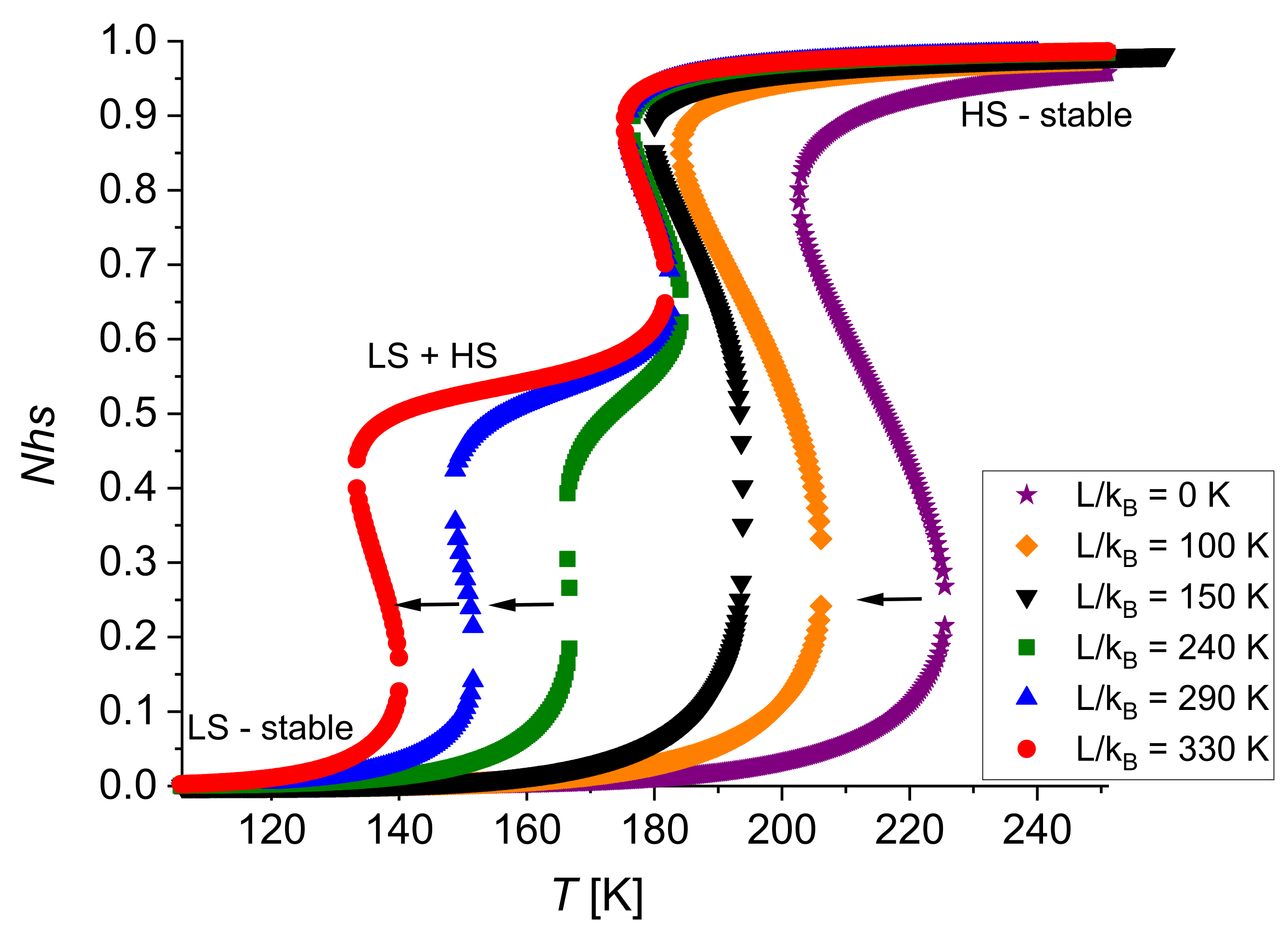
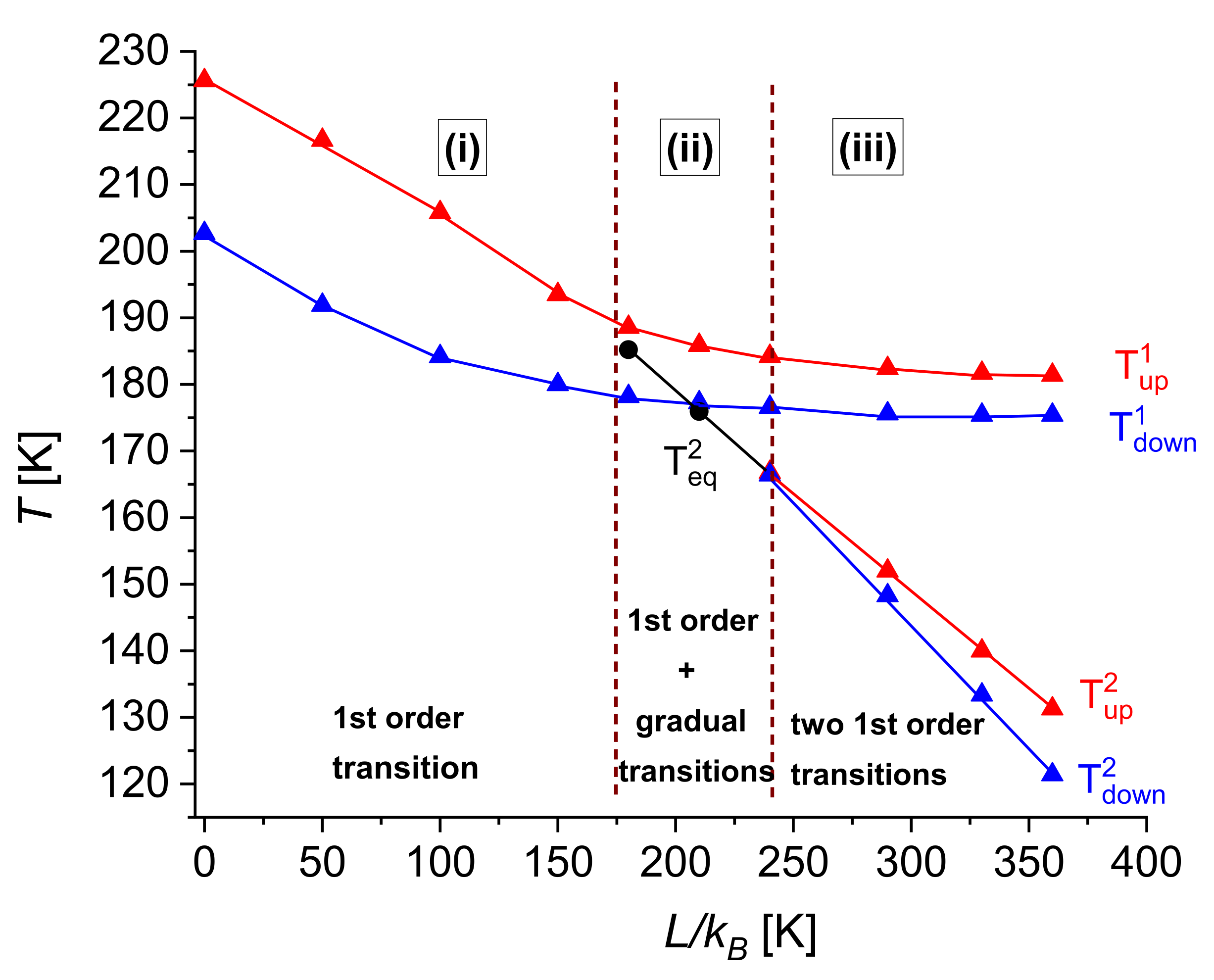
4.2. The Case ≠ 0
4.3. Size Effects under Temperature
4.4. The Case Jbs = 0
5. Conclusions
Author Contributions
Funding
Institutional Review Board Statement
Informed Consent Statement
Data Availability Statement
Acknowledgments
Conflicts of Interest
References
- Gütlich, P.; Goodwin, H.A. Spin Crossover–An Overall Perspective. In Spin Crossover in Transition Metal Compounds II; Gütlich, P., Goodwin, H., Eds.; Topics in Current Chemistry; Springer: Berlin/Heidelberg, Germany, 2004; Volume 233, pp. 1–47. [Google Scholar] [CrossRef]
- Gütlich, P.; Hauser, A.; Spiering, H. Thermal and optical switching of Iron(II) Complexes. Angew. Chem. 1994, 33, 2024–2054. [Google Scholar] [CrossRef]
- Coronado, E.; Galan-Mascaros, J.R.; Monrabal-Capilla, M.; Garcia-Martinez, J.; Parbo-Ibanez, P. Bistable Spin-Crossover Nanoparticles Showing Magnetic thermal Hysteresis near Room Temperature. Adv. Mater. 2007, 19, 1359–1361. [Google Scholar] [CrossRef]
- Hauser, A. Spin-Crossover Materials. Properties and Applications. Edited by Malcolm A. Halcrow. Angew. Chem. 2013, 52, 10419. [Google Scholar] [CrossRef]
- Ndiaye, M.; Belmouri, N.E.I.; Linares, J.; Boukheddaden, K. Elastic Origin of the Unsymmetrical Thermal Hysteresis in Spin Crossover Materials: Evidence of Symmetry Breaking. Symmetry 2021, 13, 828. [Google Scholar] [CrossRef]
- Garcia, Y.; Gütlich, P. Thermal Spin crossover in Mn(II), Mn(III), Cr(II) and Co(III) Coordination compounds. In Spin Crossover in Transition Metal Compounds II; Topics in Current Chemistry; Springer: Berlin/Heidelberg, Germany, 2004; Volume 234, pp. 49–62. [Google Scholar] [CrossRef]
- Boukheddaden, K.; Linares, J.; Tanasa, R.; Chong, C. Theoretical investigations on an axial next nearest neighour Ising-like model for spin crossover solids: One- and two-step spin transitions. J. Phys. Condens. Matter. 2007, 19, 106201–106212. [Google Scholar] [CrossRef]
- Rotaru, A.; Linares, J.; Varret, F.; Codjovi, E.; Slimani, A.; Tanasa, R.; Enachescu, C.; Stancu, A.; Haasnoot, J. Pressure effect investigated with first-order reversal-curve method on the spin-transition compounds [FexZn1−x(btr)2(NCS)2]·H2O (x = 0.6,1). Phys. Rev. B 2011, 83, 224107–224114. [Google Scholar] [CrossRef]
- Rotaru, A.; Dîrtu, M.; Enachescu, C.; Tanasa, R.; Linares, J.; Stancu, A.; Garcia, Y. Calorimetric measurements of diluted spin crossover complexes [FexM1−x(btr)2(NCS)2]•H2O with M = Zn and Ni. Polyhedron 2009, 28, 2531–2536. [Google Scholar] [CrossRef]
- Linares, J.; Jureschi, C.M.; Boukheddaden, K. Surface effects leading to unusual size dependence of the thermal hysteresis behavior in spin-crossover nanoparticles. Magnetochemistry 2016, 2, 24. [Google Scholar] [CrossRef] [Green Version]
- Constant-Machado, H.; Stancu, A.; Linares, J.; Varret, F. Thermal hysteresis loops in spin-crossover compounds analyzed in terms of classical Preisach model. IEEE Trans. Magn. 1998, 34, 2213–2219. [Google Scholar] [CrossRef]
- Krober, J.; Audière, J.P.; Claude, R.; Codjovi, E.; Kahn, O.; Hassnoot, J.; Grolière, F.; Jay, C.; Bousseksou, A.; Linares, J.; et al. Spin Transitions and Thermal Hysteresis in the Molecular-Based Materials [Fe(Htrz)2(trz)](BF4) and [Fe(Htrz)3](BF4)2.cntdot.H2O (Htrz = 1,2,4-4H-triazole; trz = 1,2,4-triazolato). Chem. Mater. 1994, 6, 1404–1412. [Google Scholar] [CrossRef]
- Linares, J.; Codjovi, E.; Garcia, Y. Pressure and Temperature Spin Crossover Sensors with Optical Detection. Sensors 2012, 12, 4479–4492. [Google Scholar] [CrossRef]
- Boukheddaden, K.; Ritti, M.H.; Bouchez, G.; Sy, M.; Dîrtu, M.M.; Parlier, M.; Linares, J.; Garcia, Y. Quantitative contact pressure sensor based on spin crossover mechanism for civil security applications. J. Phys. Chem. C 2018, 122, 7597–7604. [Google Scholar] [CrossRef]
- Kahn, O.; Martinez, C.J. Spin-Transition Polymers: From Molecular Materials Toward Memory Devices. Science 1998, 279, 44–48. [Google Scholar] [CrossRef]
- Vallone, S.P.; Tantillo, A.N.; dos Santos, A.M.; Molaison, J.J.; Kulmaczewski, R.; Chapoy, A.; Ahmadi, P.; Halcrow, M.A.; Sandeman, K.G. Giant barocaloric effect at the spin crossover transition of a molecular crystal. Adv. Mater. 2019, 31, 1807334. [Google Scholar] [CrossRef]
- Von Ranke, P.J. A microscopic refrigeration process triggered through spin-crossover mechanism. Appl. Phys. Lett. 2017, 110, 181909. [Google Scholar] [CrossRef]
- Benaicha, B.; Van Do, K.; Yangui, A.; Pittala, N.; Lusson, A.; Sy, M.; Bouchez, G.; Fourati, H.; Gomez-Garcia, C.J.; Triki, S.; et al. Interplay between spin-crossover and luminescence in a multifunctional single crystal iron(II) complex: Towards a new generation of molecular sensors. Chem. Sci. 2019, 10, 6791–6798. [Google Scholar] [CrossRef] [Green Version]
- Boukheddaden, K.; Fourati, H.; Singh, Y.; Chastanet, G. Evidence of photo-thermal effects on the first-order thermo-induced spin transition of [{Fe(NCSe)(py)2}2(m-bpypz)] spin-crossover material. Magnetochemistry 2019, 5, 21. [Google Scholar] [CrossRef] [Green Version]
- Chastanet, G.; Gaspar, A.B.; Real, J.A.; Létard, J.F. Photo-switching spin pairs synergy between liesst effect and magnetic interaction in an iron(II) binuclear spin-crossover compound. Chem. Commun. 2001, 9, 819–820. [Google Scholar] [CrossRef] [Green Version]
- Gütlich, P.; Hauser, A. Thermal and light-induced spin crossover in iron(II) complexes. Coord. Chem. Rev. 1990, 97, 1–22. [Google Scholar] [CrossRef]
- Ndiaye, M.; Boukheddaden, K. Pressure-induced multi-step and self-organized spin states in an electro-elastic model for spin-crossover solids. Phys. Chem. Chem. Phys. 2022, 24, 12870–12889. [Google Scholar] [CrossRef]
- Bousseksou, A.; Negre, N.; Goiran, M.; Salmon, L.; Tuchagues, J.P.; Boillot, M.L.; Boukheddaden, K.; Varret, F. Dynamic triggering of a spin-transition by a pulsed magnetic field. Eur. Phys. J. B 2000, 13, 451–456. [Google Scholar] [CrossRef]
- Guerroudj, S.; Caballero, R.; de Zela, F.; Jureschi, C.; Linares, J.; Boukheddaden, K. Monte Carlo–Metropolis investigations of shape and matrix effects in 2d and 3d spin-crossover nanoparticles. J. Phys. Conf. Ser. 2016, 738, 012068–012074. [Google Scholar] [CrossRef] [Green Version]
- Muraoka, A.; Boukheddaden, K.; Linares, J.; Varret, F. Two-dimensional Ising-like model with specific edge effects for spin-crossover nanoparticles: A monte Carlo study. Phys. Rev. B 2011, 84, 054119–054125. [Google Scholar] [CrossRef]
- Linares, J.; Cazelles, C.; Dahoo, P.R.; Sohier, D.; Dufaud, T.; Boukheddaden, K. Shape, size, pressure and matrix effects on 2D spin crossover nanomaterials studied using density of states obtained by dynamic programming. Comput. Mater. Sci. 2021, 187, 110061. [Google Scholar] [CrossRef]
- Singh, Y.; Oubouchou, H.; Nishino, M.; Miyashita, S.; Boukheddaden, K. Elastic-frustration-driven unusual magnetoelastic properties in a switchable core-shell spin-crossover nanostructure. Phys. Rev. B 2020, 101, 054105–054119. [Google Scholar] [CrossRef]
- Félix, G.; Mikolasek, M.; Molnár, G.; Nicolazzi, W.; Bousseksou, A. Tuning the spin crossover in nano-objects: From hollow to core–shell particles. Chem. Phys. Lett. 2014, 607, 10–14. [Google Scholar] [CrossRef]
- Slimani, A.; Khemakhem, H.; Boukheddaden, K. Structural synergy in a core-shell spin crossover nanoparticle investigated by an electroelastic model. Phys. Rev. B 2017, 95, 174104–174114. [Google Scholar] [CrossRef]
- Oubouchou, H.; Singh, Y.; Boukheddaden, K. Magnetoelastic modeling of core-shell spin-crossover nanocomposites. Phys. Rev. B 2018, 98, 014106–014119. [Google Scholar] [CrossRef]
- Enachescu, C.; Stoleriu, L.; Nishino, M.; Miyashita, S.; Stancu, A.; Lorenc, M.; Bertoni, R.; Cailleau, H.; Collet, E. Theoretical approach for elastically driven cooperative switching of spin-crossover compounds impacted by an ultrashort laser pulse. Phys. Rev. B 2017, 95, 224107–224115. [Google Scholar] [CrossRef] [Green Version]
- Fourati, H.; Ndiaye, M.; Sy, M.; Triki, S.; Chastanet, G.; Pillet, S.; Boukheddaden, K. Light-induced thermal hysteresis and high-spin low-spin domain formation evidenced by optical microscopy in a spin-crossover single crystal. Phys. Rev. B 2022, 105, 174436–174451. [Google Scholar] [CrossRef]
- Koike, M.; Murakami, K.; Fujinami, T.; Nishi, K.; Matsumoto, N.; Sunatsuki, Y. Syntheses, three types of hydrogen-bonded assembly structures, and magnetic properties of [FeIII (Him)2(hapen)]y.solvent (Him=imidazole, hapen=N,N′-bis(2-hydroxyacetophenylidene)ethylenediamine, Y=BPh4, CF3SO3, PF6, ClO4, and BF4). Inorg. Chim. Acta 2013, 399, 185–192. [Google Scholar] [CrossRef]
- Wajnflasz, J.; Pick, R. Transitions “low spin”-“high spin” dans les complexes de Fe2+. J. Phys. Colloq. 1971, 32, 91–92. [Google Scholar] [CrossRef]
- Linares, J.; Spiering, H.; Varret, F. Analytical solution of 1d Ising-like systems modified by weak long-range interaction—application to spin crossover compounds. Eur. Phys. J. B 1999, 10, 271–275. [Google Scholar] [CrossRef]
- Linares, J.; Cazelles, C.; Dahoo, P.R.; Boukheddaden, K. A first-order phase transition studied by an Ising-like model solved by entropic Sampling Monte Carlo Method. Symmetry 2021, 13, 587. [Google Scholar] [CrossRef]
- Chiruta, D.; Jureschi, C.M.; Linares, J.; Dahoo, P.R.; Garcia, Y.; Rotaru, A. On the origin of multi-step spin transition behaviour in 1d nanoparticles. Eur. Phys. J. B 2015, 88, 233. [Google Scholar] [CrossRef]
- Shteto, I.; Linares, J.; Varret, F. Monte Carlo entropic sampling for the study of metastable states and relaxation paths. Phys. Rev. E 1997, 56, 5128–5137. [Google Scholar] [CrossRef]
- Linares, J.; Enachescu, C.; Boukheddaden, K.; Varret, F. Monte Carlo entropic sampling applied to spin crossover solids: The squareness of the thermal hysteresis loop. Polyhedron 2003, 22, 2453–2456. [Google Scholar] [CrossRef]


| Size of the System | 5 × 5 | 6 × 6 | 7 × 7 |
|---|---|---|---|
| TO.D. (K) | 296 | 308 | 316 |
| (K) | 19 | 22.6 | 26 |
| System’s Size | ||||
|---|---|---|---|---|
| 5 × 5 | 25 | 9 | 16 | 0.64 |
| 6 × 6 | 36 | 16 | 20 | 0.55 |
| 7 × 7 | 49 | 25 | 24 | 0.48 |
| System’s Size | (K) | (K) |
|---|---|---|
| 5 × 5 | 10.0 | 1.0 |
| 6 × 6 | 4.4 | 7.3 |
| 7 × 7 | 0.0 | 12.5 |
Disclaimer/Publisher’s Note: The statements, opinions and data contained in all publications are solely those of the individual author(s) and contributor(s) and not of MDPI and/or the editor(s). MDPI and/or the editor(s) disclaim responsibility for any injury to people or property resulting from any ideas, methods, instructions or products referred to in the content. |
© 2023 by the authors. Licensee MDPI, Basel, Switzerland. This article is an open access article distributed under the terms and conditions of the Creative Commons Attribution (CC BY) license (https://creativecommons.org/licenses/by/4.0/).
Share and Cite
Cazelles, C.; Ndiaye, M.; Dahoo, P.; Linares, J.; Boukheddaden, K. Surface-Bulk 2D Spin-Crossover Nanoparticles within Ising-like Model Solved by Using Entropic Sampling Technique. Magnetochemistry 2023, 9, 61. https://doi.org/10.3390/magnetochemistry9030061
Cazelles C, Ndiaye M, Dahoo P, Linares J, Boukheddaden K. Surface-Bulk 2D Spin-Crossover Nanoparticles within Ising-like Model Solved by Using Entropic Sampling Technique. Magnetochemistry. 2023; 9(3):61. https://doi.org/10.3390/magnetochemistry9030061
Chicago/Turabian StyleCazelles, Catherine, Mamadou Ndiaye, Pierre Dahoo, Jorge Linares, and Kamel Boukheddaden. 2023. "Surface-Bulk 2D Spin-Crossover Nanoparticles within Ising-like Model Solved by Using Entropic Sampling Technique" Magnetochemistry 9, no. 3: 61. https://doi.org/10.3390/magnetochemistry9030061