
Grape-Bunch Identification and Location of Picking Points on Occluded Fruit Axis Based on YOLOv5-GAP

1
College of Engineering, South China Agricultural University, Guangzhou 510642, China
2
College of Economics and Management, South China Agricultural University, Guangzhou 510642, China
3
Foshan-Zhongke Innovation Research Institute of Intelligent Agriculture, Foshan 528010, China
4
Guangdong RuoBo Intelligent Robot Co., Ltd., Foshan 528010, China
*
Author to whom correspondence should be addressed.
Horticulturae 2023, 9(4), 498; https://doi.org/10.3390/horticulturae9040498
Submission received: 30 March 2023
/
Revised: 12 April 2023
/
Accepted: 14 April 2023
/
Published: 16 April 2023
(This article belongs to the Special Issue Smart Farming: Cutting-Edge Technologies and Robots Used in Horticultural Crops)
Abstract
:Due to the short fruit axis, many leaves, and complex background of grapes, most grape cluster axes are blocked from view, which increases robot positioning difficulty in harvesting. This study discussed the location method for picking points in the case of partial occlusion and proposed a grape cluster-detection algorithm “You Only Look Once v5-GAP” based on “You Only Look Once v5”. First, the Conv layer of the first layer of the YOLOv5 algorithm Backbone was changed to the Focus layer, then a convolution attention operation was performed on the first three C3 structures, the C3 structure layer was changed, and the Transformer in the Bottleneck module of the last layer of the C3 structure was used to reduce the computational amount and execute a better extraction of global feature information. Second, on the basis of bidirectional feature fusion, jump links were added and variable weights were used to strengthen the fusion of feature information for different resolutions. Then, the adaptive activation function was used to learn and decide whether neurons needed to be activated, such that the dynamic control of the network nonlinear degree was realized. Finally, the combination of a digital image processing algorithm and mathematical geometry was used to segment grape bunches identified by YOLOv5-GAP, and picking points were determined after finding centroid coordinates. Experimental results showed that the average precision of YOLOv5-GAP was 95.13%, which was 16.13%, 4.34%, and 2.35% higher than YOLOv4, YOLOv5, and YOLOv7 algorithms, respectively. The average positioning pixel error of the point was 6.3 pixels, which verified that the algorithm effectively detected grapes quickly and accurately.
1. Introduction
Grapes are one of the most important varieties of fruit production in the world. Xinjiang grapes, found in the three golden-grape producing areas, are thin, juicy, and nutritious and can reach 20–24% sugar content. In recent years, with the adjustment of agricultural structure, the grape industry has achieved rapid and green development with its own advantageous resources. However, as a characteristic forest and fruit advantageous industry, the harvest of grapes is still labor-intensive and involves low-efficiency manual operations. Because the maturity period of grapes is close to that of cotton, tomatoes, peppers and other crops, labor is tight and labor costs are high, thus affecting timely harvesting. The scale expansion of grape planting has not been synchronized and coordinated with the mechanization of grape harvest, which has become one of the important factors restricting the large-scale, intensive, and efficient development of the wine industry. Therefore, this study proposes a grape-detection algorithm, YOLOv5-GAP, based on YOLOv5, which can be used to quickly and accurately to detect the position of grape bunches and fruit stems. This system can provide visual technical support for harvesting institutions that conform to grape growing methods.
With the development of artificial intelligence technology, machine vision technology is more and more widely used in agricultural production and engineering fields [1,2]. Scholars at home and abroad have conducted much research on fruit-detection algorithms and the positioning method of picking points under partial occlusion, so as to realize fruit picking, automation, and intelligence [3,4,5,6].
To attain the automation and intelligence of fruit picking, the key is how to accurately identify and locate the target. Tang et al. studied the application of picking robots and vision technology in fruit picking [7]. Wu et al. proposed the YOLO-Banana model to accurately identify bananas and locate the banana fruit axis and cutting point. They improved the Bottleneck module of YOLOv5 and then used the edge-detection algorithm to segment the contour of the fruit axis to obtain the cut-off point [8,9]. Fu et al. added a detection layer by analyzing banana features, which reduced the weight and shortened the detection time [10]. Peng et al. used the transfer learning method and a stochastic gradient descent algorithm to optimize the Single Shot MultiBox Detector (SSD) algorithm and used the VGG16 model to replace the Res Net-101 model to solve, to a certain extent, the problem of low fruit recognition rate [11]. Tian et al. used the cyclic consistent countermeasure network for data enhancement and optimized the feature layer using a densely connected neural network (densenet) [12]. Sa et al. proposed a multi-modal Faster R-CNN model by combining multi-modal information through transfer learning [13]. Koirala et al. used RGB cameras and LED lights to acquire images at night, and developed a new architecture, MangoYOLO [14]. Zhao et al. compared three different backbone CenterNet models and finally proposed a CenterNet multiclass fruit-detection algorithm based on DLA-34 [15]. Bulanon et al. used image fusion technology to improve the level of fruit detection, identified fruit through machine vision technology, and then used a laser rangefinder to measure the distance, thereby realizing effective fruit detection [16,17]. Yu et al. improved Mask R-CNN to solve the problem of the poor robustness of traditional algorithms in unstructured environments [18]. For research on the location method of picking points under partial occlusion, Xiong et al. conducted a study on the location of grapes under disturbance [19]. Luo et al. used stereovision and image processing technology to identify and locate grape clusters and picking points and then completed grape size measurement and enclosure calculations [20,21,22,23]. Through the analysis of these studies, it was found that, for the location of the picking point for a covered fruit axis, most of them directly segment the image of the target to be picked, which can produce a large error in the picking-point location.
To enable a picking robot to walk autonomously in an orchard, Chen et al. combined hand-eye stereovision with the SLAM system to obtain a more detailed and accurate three-dimensional (3D) orchard map and established a new global mapping framework for orchard picking tasks [24]. At the same time, to achieve target detection at the pixel level, Wang et al. first found the approximate location of the fruit bunches at a distance and then segmented the branches of the bunches at close range [25]. Thiago et al. used Mask R-CNN to successfully detect, segment, and track grape clusters, achieving the fine separation of grape clusters from other structures in the image [26]. Kang et al. developed an automatic labeling algorithm and a LedNet algorithm to improve apple-detection performance, and improved DaSNet-v2 to achieve fruit and branch instance segmentation [27,28]. Lin et al. proposed a probability and region-based image segmentation method based on the color, depth, and shape information of spherical or cylindrical fruits and then used support vector machines to exclude false information [29]. Li et al. used the Deeplabv3 algorithm to segment RGB images for irregularly scattered fruiting branches of lychee clusters and removed fruitless branches through skeleton extraction and pruning operations to retain the main branches [30]. Finally, the spatial clustering method and principal component analysis method have been used to fit a 3D straight line using the noise of nonparametric density to determine the position of the resulting branch.
In machine vision tasks, it is sometimes necessary to count the detected fruit. Bargoti et al. applied ablation experiments and data augmentation techniques to the Faster R-CNN algorithm and used the tiling method, which effectively improves the recognition of small targets. For the detection and counting of individual fruit, watershed segmentation and Hough circle transform algorithms have been used [31,32]. Vasconez et al. solved the fruit counting problem with an improved Faster R-CNN and SSD algorithm [33]. Häni et al. combined deep learning and semi-supervised methods for fruit yield estimation [34]. Stein et al. used multisensors to identify, track, and locate fruit in orchards for accurate yield estimations [35]. Parico et al. used the YOLOv4-CSP and Deep SORT multi-object tracking algorithm to achieve fruit-detection predictions [36].
Aiming at grape detection in the wild orchard environment, this study examined green grapes in three scenarios—including sunny day, backlit, and partial occlusion—as the research objects to solve the problems of grape-bunch identification and the position determination of the picking point of partially occluded fruit axes. First, a grape-detection algorithm, YOLOv5-GAP, was proposed based on YOLOv5. Then, the digital image processing algorithm was combined with mathematical geometry to segment grape clusters identified by YOLOv5-GAP. After finding the centroid coordinates, the picking point was determined. The main contributions of this study were summarized as follows:
(1) The Conv layer of the first layer of the YOLOv5 algorithm Backbone was changed to the Focus layer, the convolution attention operation was performed on the first three C3 structures, the C3 structure layer was changed, and the Transformer in the Bottleneck module of the last layer of the C3 structure was used;
(2) On the basis of bidirectional feature fusion, jump links were added and variable weights were used to strengthen the fusion of feature information of different resolutions;
(3) The adaptive activation function was used to learn and decide whether the neuron needed to be activated, so as to realize the dynamic control of the nonlinear degree of the network;
(4) The digital image processing algorithm and mathematical geometry were combined to segment the grape cluster string recognized by YOLOv5-GAP, and the picking point was determined after finding the centroid coordinates.
2. Materials and Methods
2.1. Test Environment
The experiments in this study were based on the deep learning framework Pytorch 1.9.1, the programming language used was Python 3.8, and the operating system was Ubuntu 20.04.1 LTS. An Intel(R) Core(TM) i7-10700K @ 3.80 GHz × 16 processor, 8 GB memory, and a graphics card (NVIDIA Corp. (Santa Clara, CA, USA) TU104 [GeForce GTX 2080 SUPER], using CUDA11.1 and CUDNN8.2.0) were employed to speed up GPU operations and processing speed. The specific configuration is shown in Table 1.
2.2. Image and Data Collection
The grape dataset used in this paper was sampled in Zengcheng District, Guangzhou, where the Tropic of Cancer passes north of Zengcheng, and is affected by the tropical maritime monsoon climate of South Asia, where abundant rainfall, sufficient light time and high temperature are suitable for viticulture. On 18 May 2022 and 19 July 2022, the Redmi K30 Pro mobile device camera was used to collect pictures of sunshine rose grape varieties from different angles and directions of front light and backlight; the image resolution was 4624 × 3472 px, the distance between the camera and the fruit was kept in the range of 250~650 mm, a total of 1844 pictures were collected for the training and testing of grape-detection algorithms, and the grape images under front- and backlight are shown in Figure 1. We collected grape images, using the labeling tool to label the images; that is, we selected the grapes to be picked and obtained the grape dataset, and then 1476 pictures in the dataset were used as the training set, and 184 pictures were tested in the set.
2.3. Grape-Bunch Detection Algorithm
2.3.1. YOLOv5 Algorithm
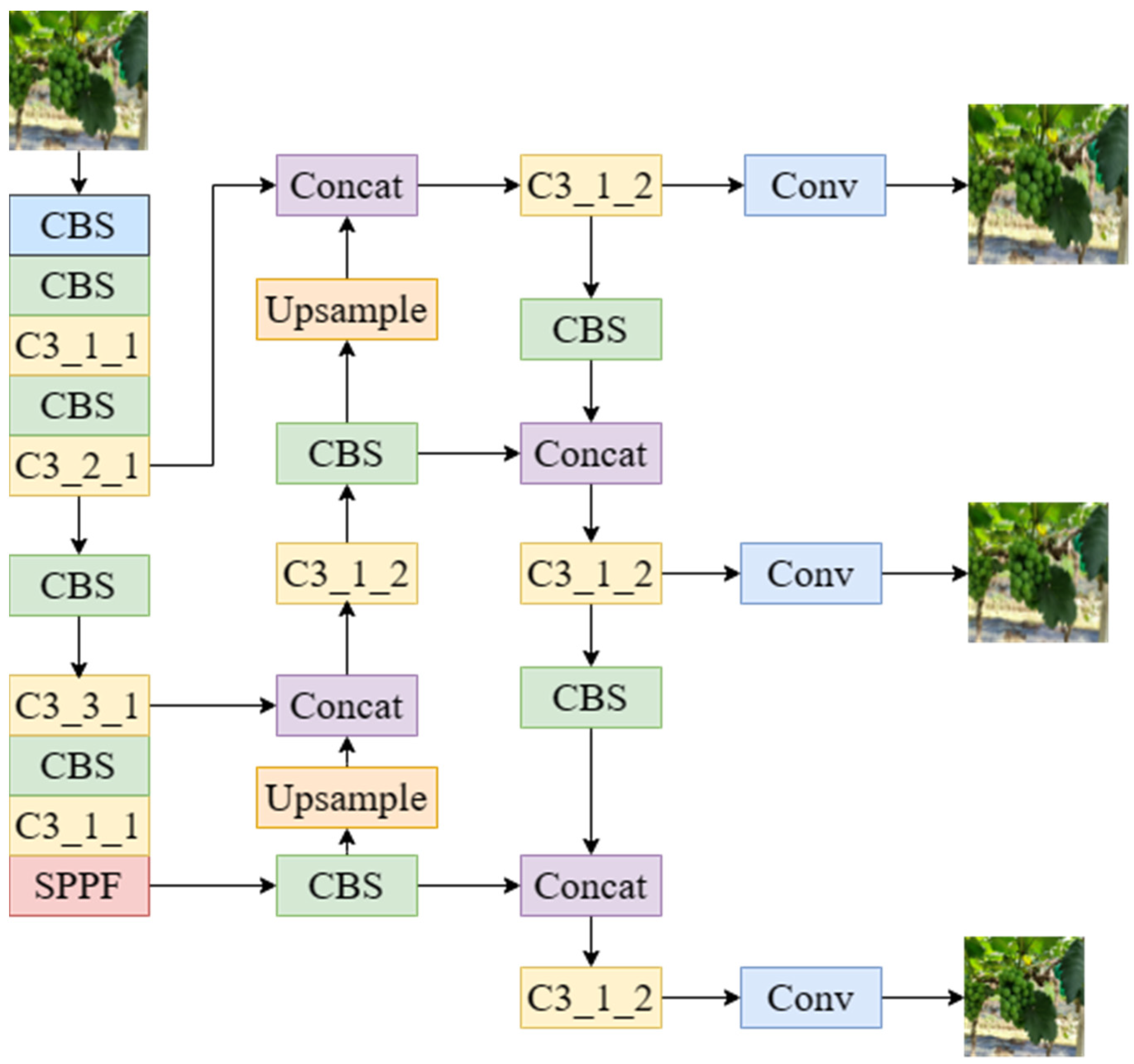
YOLOv5 is a target-detection algorithm based on regression analysis, proposed in June 2020, which reduces the stage of generating candidate regions in the two-stage detection algorithm, such that it has a faster detection speed and can achieve the purpose of real-time detection. YOLOv5 is based on the Pytorch framework. Unlike the Darknet framework, the Pytorch framework allows users to deploy and train their own datasets more quickly and easily. In the official code of YOLOv5, a total of four network models are given: YOLOv5s, YOLOv5m, YOLOv5l, and YOLOv5x. YOLOv5 is a classic single-stage algorithm structure, and the network structure of YOLOv5s-6.0 shown in Figure 2. It is mainly composed of three parts: Backbone for image feature extraction, Neck for better feature extraction using backbone, and Head for obtaining network output content using previously extracted features. In the YOLOv5 network architecture, the CBS module consists of Conv convolution, BN normalization, and SiLU activation function. Both the Backbone and Neck of YOLOv5 use a cross-stage local network (CSPNet) that allows the architecture to achieve more gradient combinations, which can allow the gradient information to produce a large correlation difference during the propagation process. Furthermore, CSPNet can reduce computation and improve inference speed and accuracy [37]. The SPPF module serially passes the input through multiple 5 × 5 MaxPool layers, with the output after each pooling becoming the input of the next pooling, and then the features are concatenated to complete the fusion.
2.3.2. Improved YOLOv5 Grape-Detection Algorithm
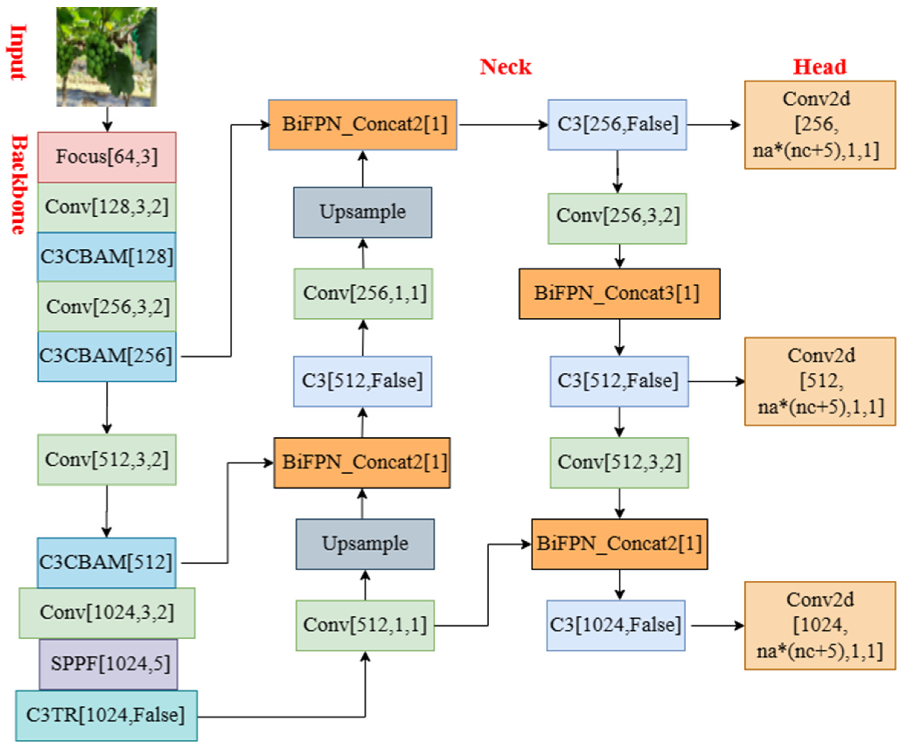
To quickly and accurately calculate the image position of grapes, it was necessary to consider the real time and accuracy of the target-detection algorithm, so as to meet the needs of efficient picking operations by picking robots. To detect grapes in a wild orchard environment more quickly and accurately, realize efficient automatic grape picking, and solve the problems of labor shortage and high labor cost, this study proposes the YOLOv5-GAP grape-detection algorithm based on the YOLOv5s-6.0 algorithm. As YOLOv5s is the network model with the smallest depth and least speed consumption in the YOLOv5 series, this study improved the grape-detection network model on the basis of YOLOv5s. The YOLOv5-GAP algorithm improved the Backbone network structure of the original algorithm, changed the Conv layer of the first layer to the Focus layer, and divided the image input into the network into several parts, which was conducive to extracting more feature information during downsampling. A convolution attention mechanism and TransformerBlock module were added, the amount of calculation was reduced to better extract global information, a more efficient weighted Bidirectional Feature Pyramid Network was proposed to fuse features of different resolutions, and an adaptive activation function was used to replace SiLU. As a result, the system could learn and decide whether to activate neurons to realize the dynamic control of the nonlinear degree of each layer of the network, so as to further improve the accuracy of the grape-detection algorithm. After the series of improvement methods mentioned above, the network structure diagram of YOLOv5-GAP, a grape-detection algorithm based on YOLOv5, was finally proposed (Figure 3).
2.3.3. Improvement of Backbone Network Structure
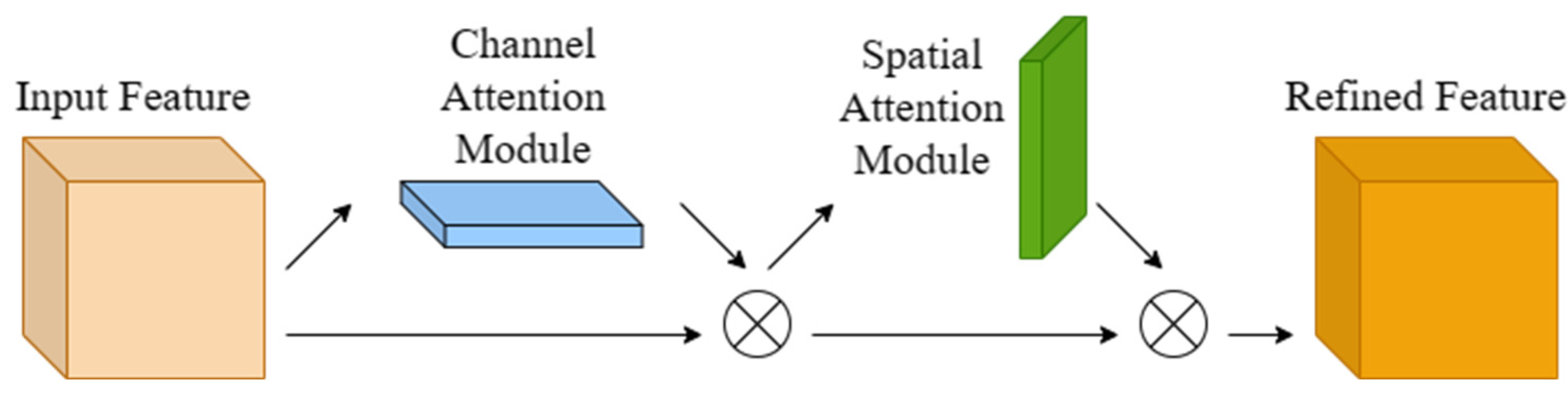
The Backbone network is usually composed of feature-extraction networks, such as ResNet [38], VGG [39], DenseNet [40], and MobileNet [41], and extracts the surface texture information, edge features, and position information of the image. To highlight the characteristics of the target and improve grape-detection accuracy, this study changed the Conv layer of the first layer of the backbone feature-extraction network CSPDarkNet53 to the Focus layer, and a convolutional attention mechanism was added to the first three C3 modules (CBAM) [42]. The attention operation was performed on the channel and spatial dimensions of the input feature, which retained more useful features than SENet’s attention mechanism, which only pays attention to the channel. The schematic diagram of the CBAM structure is shown in Figure 4.
The channel attention mechanism first compresses the input feature map F into a one-dimensional vector using average pooling and max pooling in the spatial dimension (Figure 5, channel attention module). Average and max pooling can be used to aggregate the spatial information of the feature map, and then the compressed one-dimensional vector is passed through the shared MLP. Thus, the spatial dimension was compressed, then each element was summed and merged, and finally the channel attention map Mc was generated. The channel attention mechanism was expressed as:
where represents the sigmoid functions, and ; and are the weights of the shared MLP by the two inputs; and are the average and max pooling operations on the feature map, respectively.
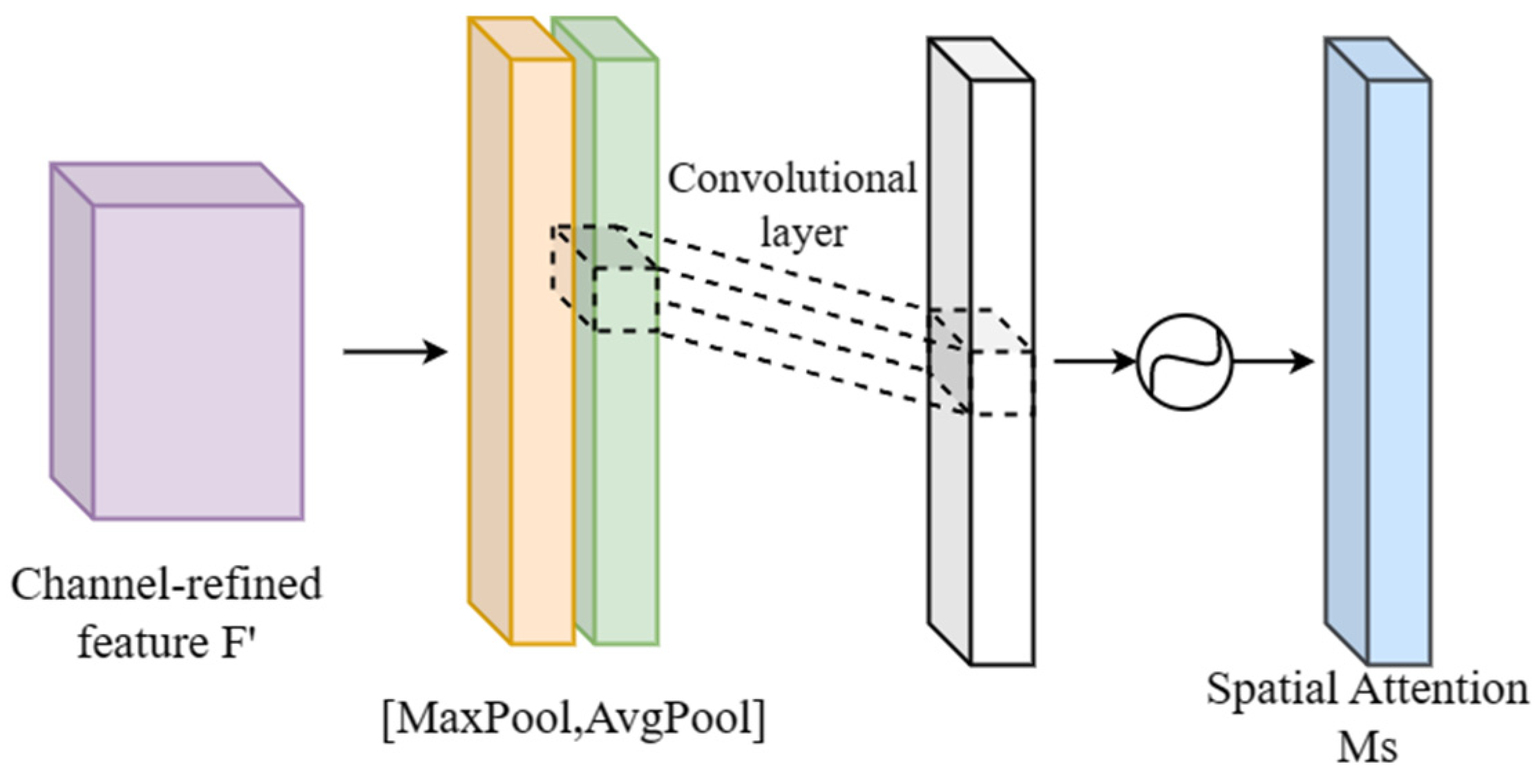
The spatial attention module is shown in Figure 6 below. The feature map F’ output by the channel attention module was used as the input feature map of this module. First, average and max pooling were performed on the input features and then the pooled results were concatenated on the channel. Then, a convolutional layer was put through to reduce its dimensionality to one. Finally, the spatial attention map Ms was generated through the sigmoid function. The spatial attention mechanism was expressed as:
where represents the sigmoid function, represents the convolution operation with a filter size of 7 × 7; and are the average and max pooling operations on the feature map, respectively.
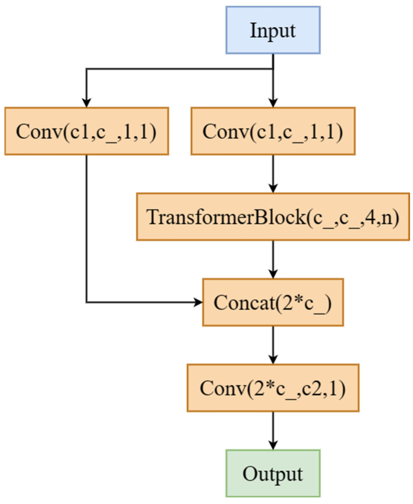
While adding the convolutional attention mechanism to the first three C3 modules of the backbone feature-extraction network CSPDarkNet53, and after moving the last layer of C3 structure to the SPPF layer, the Transformer was used in the Bottleneck module of the last layer of the C3 structure, which became the C3TR module (Figure 7).
The advantage of using the Transformer structure over RNN for machine vision tasks was that it largely solved the long-term dependency problem and could be trained in parallel [43]. The Transformer obtained an optimized feature vector by stacking the attention network and the fully connected layer, which paid attention to the relationships between each part of the sequence and other parts and the direct relationship with the partial results that were output. The improved Backbone network structure is shown in Table 2. The improved network could better extract the characteristic information of grapes.
2.3.4. Improvement of Feature Fusion Method
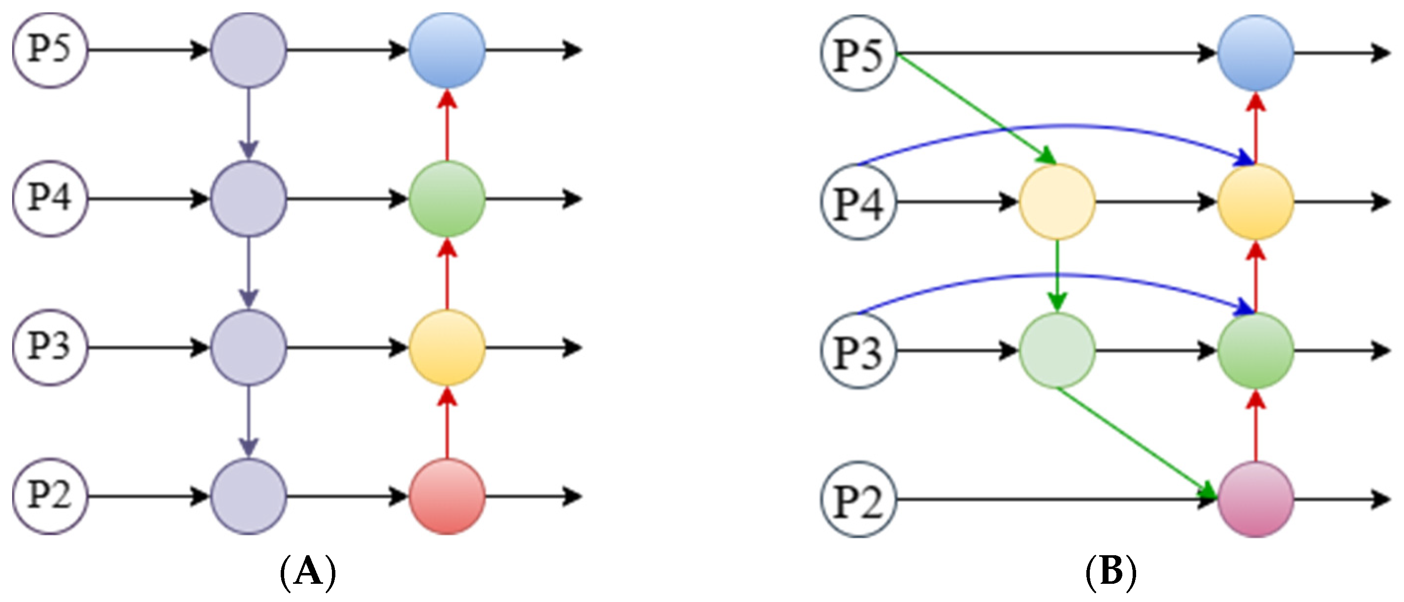
The Neck network was designed to better utilize the features extracted by the Backbone network. It reprocesses and makes reasonable use of the feature maps extracted at different stages. The Neck of the YOLOv5 algorithm adopts the path aggregation network (PANet) [44]; a schematic diagram of the structure is shown in Figure 8A. The characteristics of the PANet structure are that a top-down and bottom-up bidirectional fusion link is established at the P2 to P6 layers. Compared with the top-down fusion strategy proposed by FPN [45], PANet strengthens the underlying network Up-passing for more location information.
This study proposes to use the weighted Bidirectional Feature Pyramid Network (BiFPN) instead of PANet. To fully express different input features, BiFPN uses learnable weights to fuse input features of different resolutions [46]. In addition, the top-down and bottom-up fusion strategies in PANet were used for reference and the feature fusion was repeated many times. BiFPN added skip links in the same layer and considered that when a node had only one input edge the contribution to feature fusion was small. BiFPN deleted nodes with only one input edge, which did not bring too much computational cost, and thus more features were fused. The schematic diagram of the structure is shown in Figure 8B.
2.3.5. Improvement of Activation Function
In the neural network, the output of each layer is the linear function of the input of the previous layer, but the expression ability of the linear model was not sufficient, such that the activation function was introduced to improve the nonlinear expression ability of the model. The CBS module in the YOLOv5 algorithm used the SiLU activation function for activation, expressed in Equation (3) as:
In this study, the adaptive activation function Meta-ACON was used instead of SiLU. The Meta-AconC activation function can learn independently and decide whether neurons needed to be activated, so as to realize the dynamic control of the degree of nonlinearity of the network. After the activation function was replaced, the CBS module responded accordingly and became the CBM module. The expression of the Meta-AconC activation function is shown in Equation (4), expressed as:
where p1 and p2 are responsible for the upper and lower limits of the control function and the parameter responsible for dynamically controlling the linearity/nonlinearity of the activation functions, and , to save parameters.
2.4. Model Training
Before the grape dataset was input into the YOLOv5 network model for training, the data augmentation method included in the algorithm was used to enrich the dataset. Various methods such as random scaling, random cropping, and image resizing were used to stitch the images, which not only expanded the image set but also improved the detection of small targets. In addition, before training the model, the grape image was adaptively scaled and filled, and the input image size was normalized to 640 × 640 pixels.
In the algorithm training phase, nine anchor boxes of different sizes were set. During the training process, the stochastic gradient descent (SGD) algorithm was used to optimize the algorithm. The momentum size of the momentum optimizer was set to 0.937, the attenuation coefficient was 0.0005, and the number of target categories was 1. The number of training iterations was 150, the number of samples input for each iteration was 8, and the algorithm with the best detection effect was selected as the grape-detection algorithm. A total of 9 algorithms were trained in this experiment, which included YOLOv4, YOLOv5, YOLOv7, YOLOv5-GAP, and 5 ablation test algorithms of YOLOv5-GAP.
2.5. Picking-Point Positioning
After grape bunches were detected using the proposed YOLOv5-GAP algorithm, it was necessary to further determine the picking-point locations. However, the fruit stems of the grapes were blocked by branches and leaves and the overall shape was similar to the main vine, such that it was not suitable to use the deep learning method directly. This study used the digital image processing algorithm combined with mathematical geometry to locate the picking points. The difficulty in locating the picking point lay in how to accurately find the growth direction of the fruit stem. The geometric shape of the grape bunches was mostly long conical and affected by gravity. The fruit stem is generally vertically downward and the picking point on the fruit bunch is above the center. However, some fruit stems are not in the center of the fruit bunch, in which case, there may be an error in positioning the picking point directly above the center of the fruit bunch. In this study, the picking point was determined by the centroid. First, the grape clusters were identified by the YOLOv5-GAP algorithm and then the centroid of the fruit cluster was obtained through a series of digital image processing algorithms. The fruit axis was usually above the centroid of the fruit cluster and the centroid and upper boundary was in the vertical direction. The intersection point was defined as the lower extreme point of the fruit stem and the position 10 pixels directly above the lower extreme point was used as the picking point. Here, 40 sample images were used to locate the picking point on the fruit axis.
2.5.1. Image Segmentation
Grape image segmentation is the basis for finding picking points. First, the YOLOv5-GAP algorithm proposed in this study was used to identify grape bunches to reduce noise; a detected image is shown in Figure 9. However, the recognized original image still contained the influence of some green leaves, branches, and other sundries. Here, the original image was converted to HSV color space and binary images of grape bunches were obtained. Then, the isolated noise pixels were processed by a median filter, which did not cause obvious blur to the image and maintained the edge characteristics of the image.
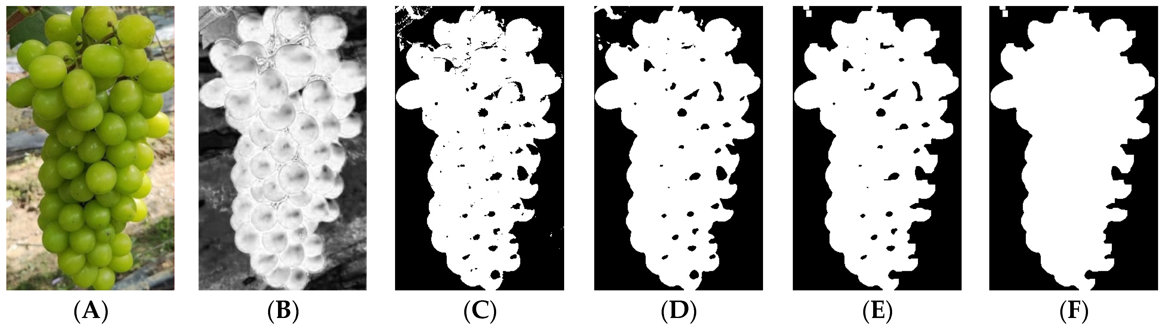
The open operation in mathematical morphology can smooth the contours of an image, break narrow connections, and eliminate burrs. The filtered binary image noise here was mainly composed of surrounding noise blocks and inner noise holes. For noise blocks, the morphological opening operation was used to eliminate part of the influence. The findContours function for internal noise holes was used to select the RETR_CCOMP mode, find the contour of the hole in the grape bunch, judge the size of each contour, and fill it when it was <60 pixels; the image segmentation process is shown in Figure 10. After image segmentation, some green leaves might be separated from the overall outline of the grape. However, the size of these green leaves was negligible.
2.5.2. Geometric Calculation of Picking-Point Position
The binary image after morphological operation segmented the grape bunches well, with the fruit bunch area displayed as white (pixel value 1) and the rest of the area displayed as black (pixel value 0). However, to find the centroid of an irregularly shaped bunch of grapes, the center of a blob needed to be determined, which was a group of interconnected pixels with the same properties in an image. In this study, OpenCV was used to find the center of a binary blob.
In image processing, each shape is composed of pixels and the centroid is the weighted average of all the pixels that make up the shape. OpenCV uses moments to find the center of a blob. Image moments are a special weighted average of image pixel intensities that can be used to calculate the radius, area, and centroid [47]. The centroid was calculated using Equation (5), expressed as:
where Cx is the x-coordinate of the center of mass, Cy the y-coordinate of the center of mass, and M the moment.
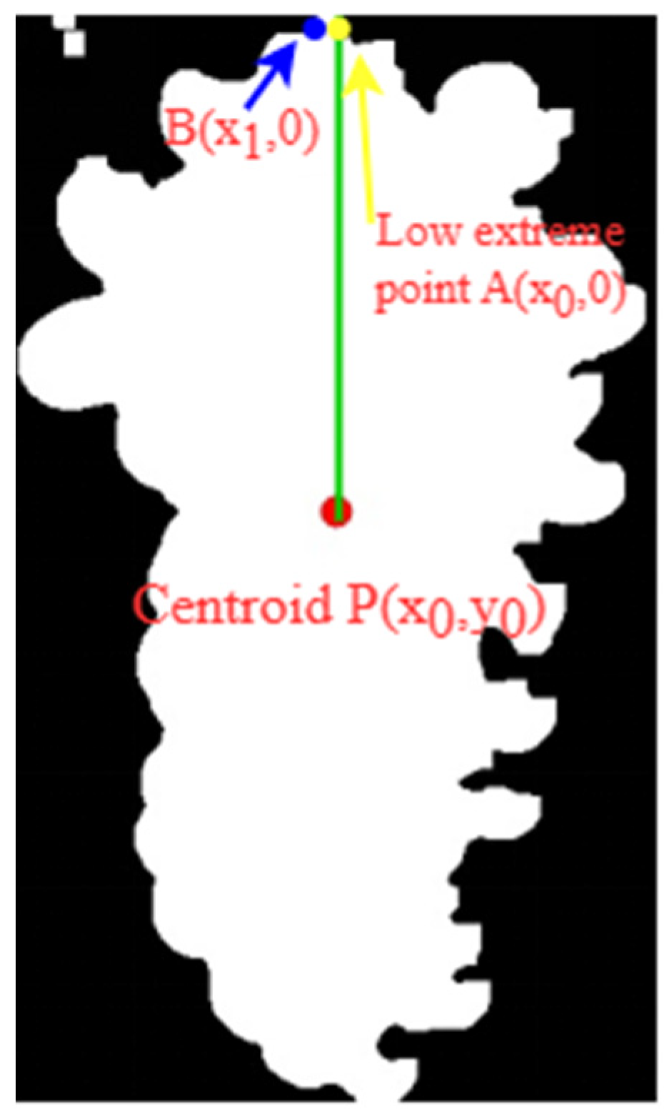
The centroid of the grape bunch obtained through the above calculation is shown in Figure 11. The P coordinate of the centroid was (x0, y0) and, when the fruit axis pointed vertically downward, it was usually above the centroid of the bunch. Here, A(x0,0) directly above the centroid P(x0, y0) was taken as the lower extreme point of the fruit stem, the position 10 pixels directly above the lower extreme point was the picking point, and the position coordinates of the picking point were (x0, −10). Notably, the lower extreme point of the actual fruit stem was B(x1,0), such that Equation (6) for the pixel error value of the lower extreme point was:
When picking, the accuracy of the axial dimension of the cut fruit shaft belonged to the free precision range, but in actual scenarios, some fruit stems were not vertically downward and had a certain angle. Considering the fault tolerance of the end mechanism, when the error of the extreme point under the fruit stem was within the allowable range, the detection of the grape-bunch axis by the end mechanism had a certain robustness.
3. Results
3.1. Algorithm Evaluation Indicators
These experiments used precision (P), recall (R), average precision (AP), Fβ score [48], and model weight size as the evaluation metrics for the algorithm. Among these, the AP was the area under the P-R curve and the Fβ score was the balance of P (the proportion of positive samples that were correctly predicted of all detected samples) and the R metric (the proportion of all positive samples). In this experiment, β = 2 was taken to calculate the Fβ score. The specific calculation equations of the above evaluation indicators are shown in Equations (7)–(10), expressed as:
where TP is the number of positive samples predicted as positive by the algorithm, FP is the number of negative samples predicted as positive by the algorithm, and FN is the number of positive samples predicted as negative by the algorithm.
In this paper, the Intersection over Union (IOU) ratio between the prediction results and the real target label was used to determine whether the detected target was grapes. When the value of the IOU is greater than the set threshold, it was considered to have successfully detected grapes, and the calculation of the IOU can be expressed by Equation (11). The IOU was set to 0.55 during the experiment in this article.
For the object-detection model, we generally used the final output of a confidence level, by setting a confidence threshold—for example, this paper sets the confidence threshold to 0.6, and then higher than 0.6 was considered to be detected as a positive sample. Then, on the basis of this set of positive samples, we set an IOU threshold (the IOU threshold of this paper is 0.55) greater than the threshold considered to be TP, and the others were considered to be FP.
3.2. Algorithm Training Results
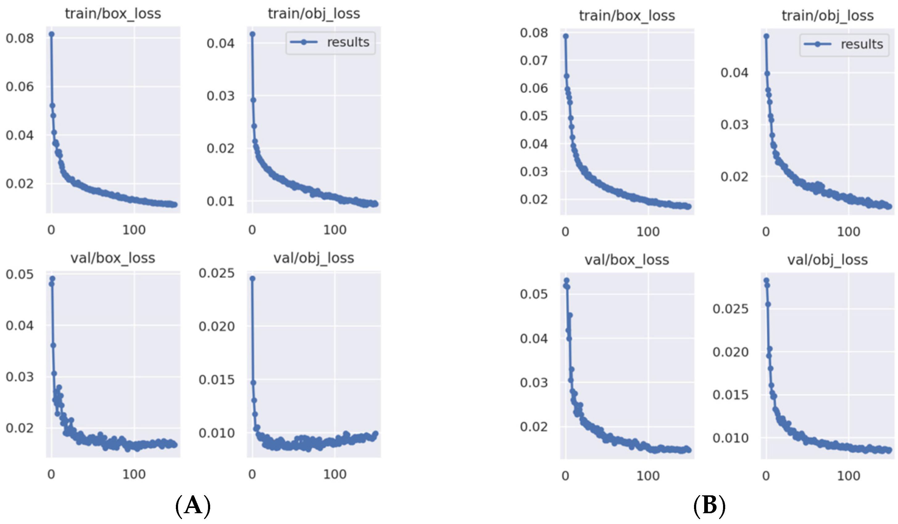
The divided training and validation sets were input into the YOLOv5 and YOLOv5-GAP networks for training. After 150 batches of training, the obj loss and box loss function value curves during training were obtained (Figure 12).
The box loss value of the YOLOv5 algorithm decreased rapidly between training batches 0 and 20, and then the decline rate slowed (Figure 12). After the improvement of YOLOv5-GAP and applying the training set after 150 training cycles, the box loss value was slightly larger than the box loss value of the YOLOv5 algorithm. However, the box loss value of YOLOv5-GAP on the validation set was smaller than that of YOLOv5, and it finally stabilized around 0.015 (Figure 12). When the training batch was between 0 and 50, the obj loss value of YOLOv5 on the validation set decreased, but after 50 batches, the loss value volatility increased. Meanwhile, the obj loss value of the YOLOv5-GAP on the validation set decreased steadily, and the final loss value stabilized around 0.008.
3.3. Ablation Test Results and Analysis
To clearly examine the impact of each improvement point on the algorithm, incremental ablation experiments were used to verify a test set of 184 grape images (Table 3). Algorithm A represented the original YOLOv5 algorithm, Algorithm B represented the replacement of the first Conv layer in the Backbone of the original YOLOv5 algorithm with Focus; Algorithm C, with the basis of Algorithm B, represented the first three C3 structures of the Backbone of the original YOLOv5 algorithm, with attention paid to the channel and space dimensions; Algorithm D, on the basis of Algorithm C, represented the situation after moving the last layer of the Backbone C3 structure to the SPPF layer, and the original Bottleneck of the last layer of C3 structure being replaced by the Transformer-Block module, becoming a TR structure; Algorithm E, on the basis of Algorithm D, represented a weighted Bidirectional Feature Pyramid Network (BiFPN) proposed to perform more-efficient multi-scale feature fusion; and the YOLOv5-GAP Algorithm F proposed here, based on Algorithm E, represented using the Meta-ACON activation function to replace SiLU. Compared with Algorithm A, the P rate, R rate, and AP rate of Algorithm B were increased by 0.61%, 1.19%, and 0.88%, respectively, which yielded that the algorithm was more accurate in identifying grapes. Although the accuracy of Algorithm C was significantly different from that of Algorithm A and B, the R rate was 2.07% higher than that of Algorithm A, which showed that the CBAM module effectively improved the R rate. Algorithm D improved the accuracy of Algorithm C after using the Transformer module. Algorithm E slightly improved the AP rate of the model. The P rate of YOLOv5-GAP Algorithm F proposed here was 1.74% lower than that of Algorithm E, but the R rate, AP rate, and Fβ scores were the highest, at 97.34%, 95.13%, and 0.9331, respectively, and the weight only increased by 0.5 M, compared with the original model. This demonstrated that YOLOv5-GAP better balanced the P rate, R rate, AP rate, Fβ score, and weight, which effectively improved effective grape detection.
3.4. Comparative Test Results and Analysis
The effectiveness of the YOLOv5-GAP algorithm for grape detection was further verified under the same experimental conditions in comparison with the existing mainstream single-stage target-detection algorithm. The experiment utilized P rate, R rate, AP rate, Fβ score, and weight size as evaluation indicators for algorithm performance. The performance comparison results of different detection algorithms are shown in Table 4.
The YOLOv4 algorithm, with the same dataset, had the highest precision rate for grape detection, with a precision rate of 90.32% (Table 4). However, its R rate was the lowest and the weight of YOLOv4 reached 244 M, which affected the inference speed. The AP rate of YOLOv5-GAP was 95.13%, which was 16.13%, 4.34%, and 2.35% higher than that of YOLOv4, YOLOv5, and YOLOv7, respectively. The YOLOv5-GAP algorithm proposed here achieved the highest Fβ score, reaching 0.9331, which indicated that it offered a better balance of detection precision and recall and could meet the requirements of efficient grape detection.
3.5. Comparison of Test Results
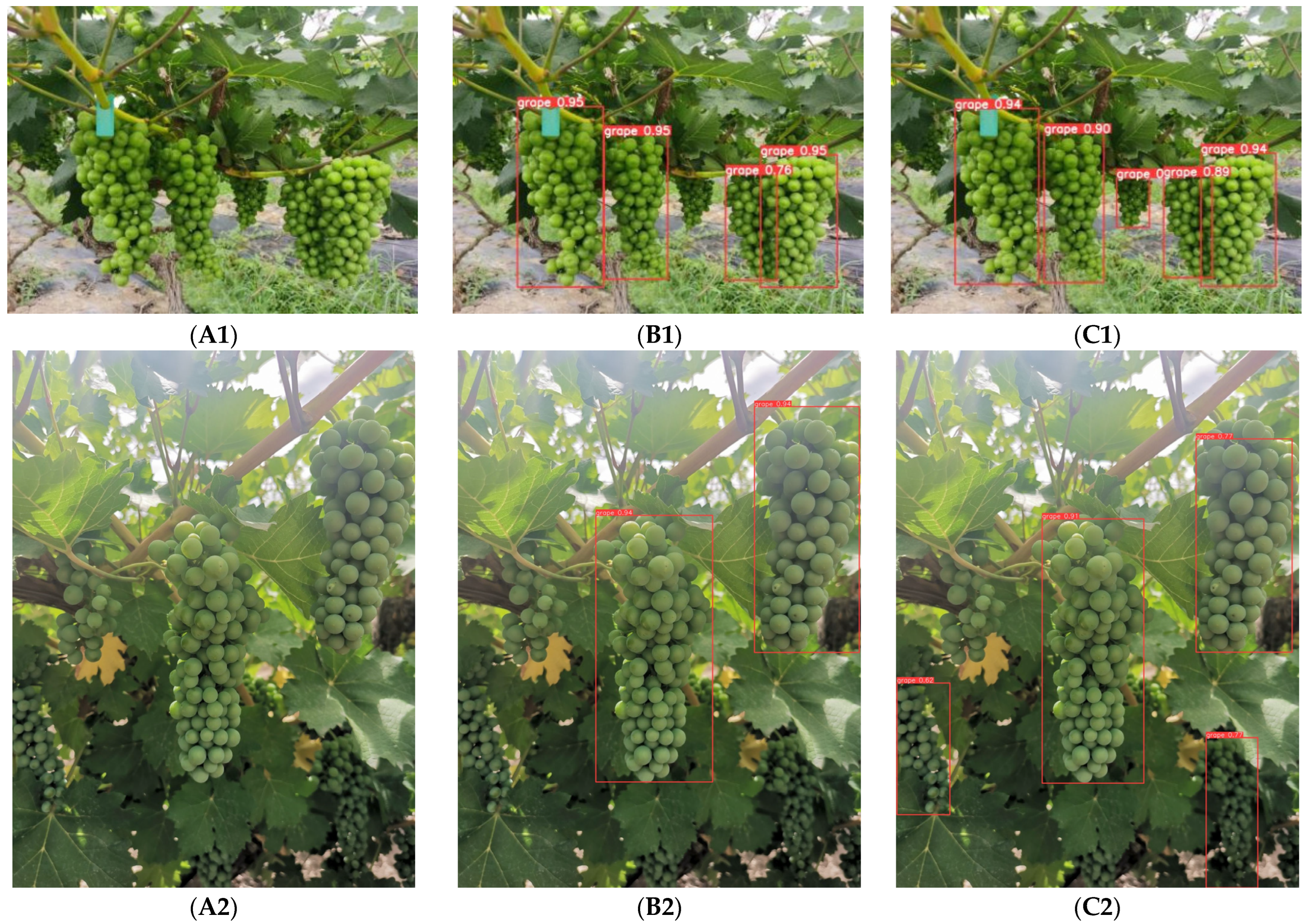
In this paper, the grape pictures of Zengcheng District, Guangzhou (Figure 13(A1)), and the grape pictures of Babao Baron Winery, Shihezi, Xinjiang (Figure 13(A2)), were tested, respectively, and compared with the original YOLOv5 network, to demonstrate the detection effect of the YOLOV5-GAP algorithm on grapes. The test results are shown in Figure 13.
The YOLOv5-GAP algorithm detected some occluded, shadowed, and overlapping grape clusters (Figure 13). Compared with YOLOv5, the missed detection of grape clusters was significantly improved. Therefore, the YOLOv5-GAP proposed here had the better detection performance.
3.6. Picking-Point Positioning-Error Test
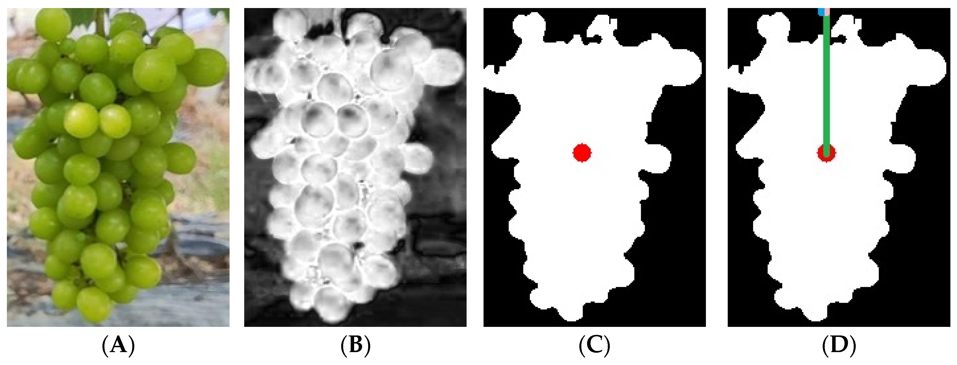
Here, 40 sample pictures were selected for the picking-point location experiment. The intersection of the centroid and upper boundary in the vertical direction was defined as the lower extreme point of the fruit stem. A positioning process image of the lower extreme point is shown in Figure 14, and due to the complex background, most of the short fruit axes were obscured. The problem of finding picking-point locations when the fruit axes are partially obscured was discussed above. Here, grape clusters were detected by the improved YOLOv5, the geometric algorithm was then used to estimate the position of the fruit axis, and the fruit-axis picking point with pixel error was calculated.
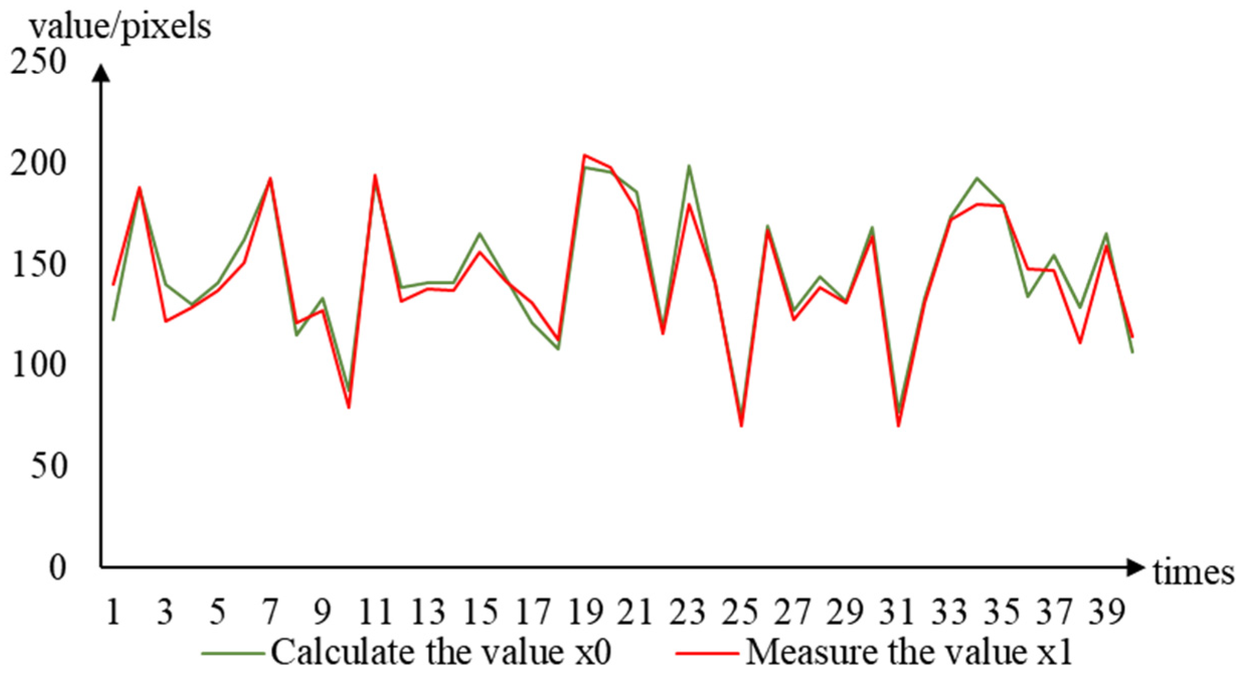
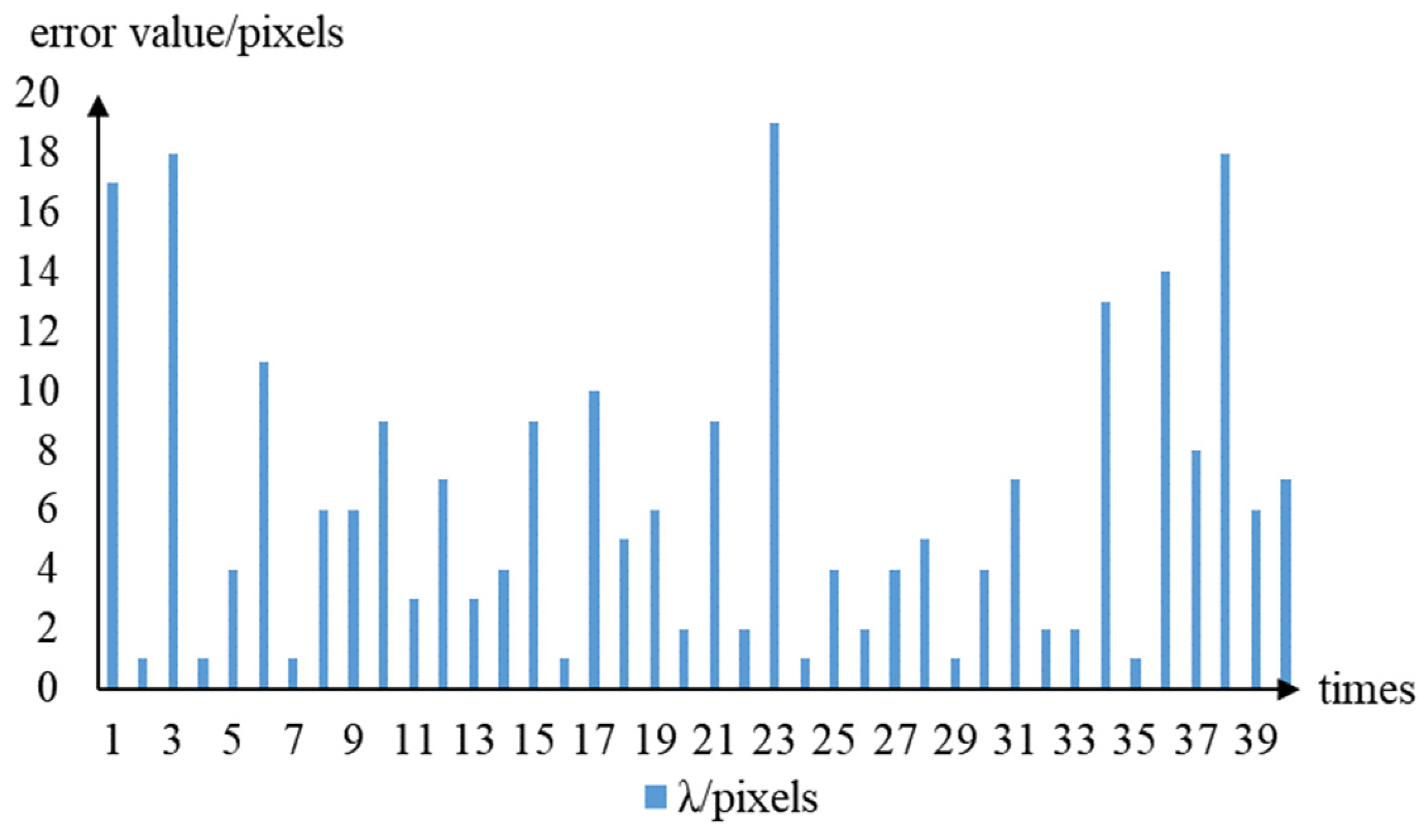
Assuming that the position 10 pixels directly above the lower extreme point was used as the picking point, the positioning error of the picking point was mainly derived from the pixel positioning error of the lower extreme point. First, the position of the extreme point under the grape cluster axis was manually measured, the algorithm proposed here was then used for calculation and comparison, and the error was estimated. The position of the lower extreme point measured manually was marked as (x1, 0), and the calculated position was marked as (x0, 0) (Figure 15). Thus, the pixel error value of the lower extreme point was calculated according to Equation (6), λ = |x1 – x0|. The pixel error of the lower extreme points of the 40 sample images is shown in Figure 16.
By analyzing the pixel error value of the lower extreme point positioning (Figure 16), the average pixel positioning error of the lower extreme point of the fruit stalk was used to determine the picking point at 6.3 pixels. Of these images, 33 images had pixel error values below 10 pixels and the pixel errors of the lower extreme points of the other 7 images were greater than 10 pixels, with the lower extreme point located in the area outside the fruit stalk. The analysis of the extreme point calculation method used here showed that it might be that some green branches and leaves and adjacent grape clusters interfered with centroid calculation during image segmentation. The fault tolerance of the picking robot end mechanism of this system was >10 pixels, which could make up for the direction pixel error generated by the method used here.
4. Conclusions
In view of the characteristics of a wild orchard environment, to quickly and accurately calculate the image position and picking point of grapes, a grape-detection algorithm, YOLOv5-GAP, was proposed based on YOLOv5. This algorithm integrated the network structure of YOLOv5’s Backbone and feature fusion method, and the activation function was improved for grape-detection performance. The digital image processing algorithm combined with mathematical geometry was used to locate the picking point.
Compared with the original YOLOv5 algorithm, the average precision of YOLOv5-GAP was 95.13%, which was 4.34% higher than the average precision of YOLOv5, and the Fβ score was improved by 3.39%. The detection performance was better than the single-stage target-detection algorithms YOLOv4, YOLOv5, and YOLOv7. The average pixel positioning error of the extreme point under the fruit stalk used to determine the picking point was 6.3 pixels, which verified that the algorithm was effective in grape detection.
The YOLOv5-GAP algorithm proposed here was not ideal for the detection of some small-target grape clusters in shadows. In the future, the network model structure will be further optimized to improve the detection performance of small-target grape clusters in shadows and an end mechanism will be developed that meets the picking-point positioning method proposed in this study. At the same time, to enable the grape harvester to walk in the orchard independently, the harvester will be positioned by a visual odometer in the next step.
Author Contributions
Conceptualization, T.Z. and X.Z.; Data curation, T.Z. and X.Z.; Formal analysis, T.Z. and M.W.; Funding acquisition, X.Z.; Investigation, T.Z., F.W., M.W., Z.C., L.L. and X.Z.; Methodology, T.Z.; Project administration, L.L. and X.Z.; Resources, T.Z., F.W., M.W., Z.C., L.L. and X.Z.; Software, T.Z.; Supervision, L.L. and X.Z.; Validation, T.Z. and M.W.; Visualization, T.Z.; Writing—original draft, T.Z.; Writing—review and editing, T.Z. and X.Z. All authors have read and agreed to the published version of the manuscript.
Funding
This research was funded by Research on the Harvesting Mechanism of Wine Grapes based on Visual Navigation (2022DB004), Guangdong Foshan Science and Technology Innovation Project (2120001008424), and Provincial Science and Technology Department Funding Project of Jiangxi, China (20212ABC03A27).
Data Availability Statement
The data presented in this study are available on request from the corresponding author.
Acknowledgments
The authors would like to thank the anonymous reviewers for their critical comments and suggestions for improving the manuscript.
Conflicts of Interest
The authors declare no conflict of interest.
References
- Chen, S.; Zou, X.; Zhou, X.; Xiang, Y.; Wu, M. Study on fusion clustering and improved yolov5 algorithm based on multiple occlusion of camellia oleifera fruit. Comput. Electron. Agric. 2023, 206, 107706. [Google Scholar] [CrossRef]
- Tang, Y.; Huang, Z.; Chen, Z.; Chen, M.; Zhou, H.; Zhang, H.; Sun, J. Novel visual crack width measurement based on backbone double-scale features for improved detection automation. Eng. Struct. 2023, 274, 115158. [Google Scholar] [CrossRef]
- Tang, Y.; Zhou, H.; Wang, H.; Zhang, Y. Fruit detection and positioning technology for a camellia oleifera c. Abel orchard based on improved yolov4-tiny model and binocular stereo vision. Expert Syst. Appl. 2023, 211, 118573. [Google Scholar] [CrossRef]
- Bac, C.W.; Hemming, J.; van Henten, E.J. Stem localization of sweet-pepper plants using the support wire as a visual cue. Comput. Electron. Agric. 2014, 105, 111–120. [Google Scholar] [CrossRef]
- Kalampokas, Τ.; Vrochidou, Ε.; Papakostas, G.A.; Pachidis, T.; Kaburlasos, V.G. Grape stem detection using regression convolutional neural networks. Comput. Electron. Agric. 2021, 186, 106220. [Google Scholar] [CrossRef]
- Tang, Y.; Qiu, J.; Zhang, Y.; Wu, D.; Cao, Y.; Zhao, K.; Zhu, L. Optimization strategies of fruit detection to overcome the challenge of unstructured background in field orchard environment: A review. Precis. Agric. 2023, 24, 1–37. [Google Scholar] [CrossRef]
- Tang, Y.; Chen, M.; Wang, C.; Luo, L.; Li, J.; Lian, G.; Zou, X. Recognition and localization methods for vision-based fruit picking robots: A review. Front. Plant Sci. 2020, 11, 510. [Google Scholar] [CrossRef]
- Wu, F.; Duan, J.; Ai, P.; Chen, Z.; Yang, Z.; Zou, X. Rachis detection and three-dimensional localization of cut off point for vision-based banana robot. Comput. Electron. Agric. 2022, 198, 107079. [Google Scholar] [CrossRef]
- Wu, F.; Duan, J.; Chen, S.; Ye, Y.; Ai, P.; Yang, Z. Multi-target recognition of bananas and automatic positioning for the inflorescence axis cutting point. Front. Plant Sci. 2021, 12, 705021. [Google Scholar] [CrossRef]
- Fu, L.; Wu, F.; Zou, X.; Jiang, Y.; Lin, J.; Yang, Z.; Duan, J. Fast detection of banana bunches and stalks in the natural environment based on deep learning. Comput. Electron. Agric. 2022, 194, 106800. [Google Scholar] [CrossRef]
- Peng, H.; Huang, B.; Shao, Y.; Li, Z.; Zhang, C.; Chen, Y.; Xiong, J. General improved SSD model for picking object recognition of multiple fruits in natural environment. Trans. Chin. Soc. Agric. Eng. 2018, 34, 155–162. [Google Scholar]
- Tian, Y.; Yang, G.; Wang, Z.; Li, E.; Liang, Z. Detection of Apple Lesions in Orchards Based on Deep Learning Methods of CycleGAN and YOLOV3-Dense. J. Sens. 2019, 2019, 1–13. [Google Scholar] [CrossRef]
- Sa, I.; Ge, Z.; Dayoub, F.; Upcroft, B.; Perez, T.; McCool, C. DeepFruits: A Fruit Detection System Using Deep Neural Networks. Sensors 2016, 16, 1222. [Google Scholar] [CrossRef] [PubMed]
- Koirala, A.; Walsh, K.B.; Wang, Z.; McCarthy, C. Deep learning for real-time fruit detection and orchard fruit load estimation: Benchmarking of ‘MangoYOLO’. Precis. Agric 2019, 20, 1107–1135. [Google Scholar] [CrossRef]
- Zhao, K.; Yan, W.Q. Fruit Detection from Digital Images Using CenterNet. In Geometry and Vision; ISGV 2021. Communications in Computer and Information Science; Nguyen, M., Yan, W.Q., Ho, H., Eds.; Springer: Cham, Switzerland, 2021; Volume 1386. [Google Scholar] [CrossRef]
- Bulanon, D.M.; Burks, T.F.; Alchanatis, V. Image fusion of visible and thermal images for fruit detection. Biosyst. Eng. 2009, 103, 12–22. [Google Scholar] [CrossRef]
- Bulanon, D.M.; Kataoka, T. Fruit detection system and an end effector for robotic harvesting of Fuji apples. Agric Eng Int CIGR J. 2010, 12, 203–210. [Google Scholar]
- Yu, Y.; Zhang, K.; Yang, L.; Zhang, D. Fruit detection for strawberry harvesting robot in non-structural environment based on Mask-RCNN. Comput. Electron. Agric. 2019, 163, 104846. [Google Scholar] [CrossRef]
- Xiong, J.; He, Z.; Lin, R.; Liu, Z.; Bu, R.; Yang, Z.; Peng, H.; Zou, X. Visual positioning technology of picking robots for dynamic litchi clusters with disturbance. Comput. Electron. Agric. 2018, 151, 226–237. [Google Scholar] [CrossRef]
- Luo, L.; Tang, Y.; Zou, X.; Ye, M.; Feng, W.; Li, G. Vision-based extraction of spatial information in grape clusters for harvesting robots. Biosyst. Eng. 2016, 151, 90–104. [Google Scholar] [CrossRef]
- Luo, L.; Tang, Y.; Lu, Q.; Chen, X.; Zhang, P.; Zou, X. A vision methodology for harvesting robot to detect cutting points on peduncles of double overlapping grape clusters in a vineyard. Comput. Ind. 2018, 99, 130–139. [Google Scholar] [CrossRef]
- Luo, L.; Liu, W.; Lu, Q.; Wang, J.; Wen, W.; Yan, D.; Tang, Y. Grape berry detection and size measurement based on edge image processing and geometric morphology. Machines 2021, 9, 233. [Google Scholar] [CrossRef]
- Luo, L.; Zou, X.; Wang, C.; Chen, X.; Yang, Z.; Situ, W. Recognition method for two overlaping and adjacent grape clusters based on image contour analysis. Nongye Jixie Xuebao/Trans. Chin. Soc. Agric. Mach. 2017, 48, 15–22. [Google Scholar]
- Chen, M.; Tang, Y.; Zou, X.; Huang, Z.; Zhou, H.; Chen, S. 3D global mapping of large-scale unstructured orchard integrating eye-in-hand stereo vision and SLAM. Comput. Electron. Agric. 2021, 187, 106237. [Google Scholar] [CrossRef]
- Wang, H.; Lin, Y.; Xu, X.; Chen, Z.; Wu, Z.; Tang, Y. A Study on Long–Close Distance Coordination Control Strategy for Litchi Picking. Agronomy 2022, 12, 1520. [Google Scholar] [CrossRef]
- Thiago, T.; Leonardo, S.; de Souza, L.; Santos, A.A.D.; Avila, S. Grape detection, segmentation, and tracking using deep neural networks and three-dimensional association. Comput. Electron. Agric. 2020, 170, 105247. [Google Scholar]
- Hanwen, K.; Chao, C. Fast implementation of real-time fruit detection in apple orchards using deep learning. Comput. Electron. Agric. 2019, 168, 105108. [Google Scholar]
- Kang, H.; Chen, C. Fruit detection, segmentation and 3D visualisation of environments in apple orchards. Comput. Electron. Agric. 2020, 171, 105302. [Google Scholar] [CrossRef]
- Lin, G.; Tang, Y.; Zou, X.; Xiong, J.; Fang, Y. Color-, depth-, and shape-based 3D fruit detection. Precis. Agric. 2020, 21, 1–17. [Google Scholar] [CrossRef]
- Li, J.; Tang, Y.; Zou, X.; Lin, G.; Wang, H. Detection of Fruit-Bearing Branches and Localization of Litchi Clusters for Vision-Based Harvesting Robots. IEEE Access 2020, 8, 117746–117758. [Google Scholar] [CrossRef]
- Bargoti, S.; Underwood, J. Deep Fruit Detection in Orchards. arXiv 2016, arXiv:1610.03677. [Google Scholar]
- Bargoti, S.; Underwood, J.P. Image Segmentation for Fruit Detection and Yield Estimation in Apple Orchards(Article). J. Field Robot. 2017, 34, 1039–1060. [Google Scholar] [CrossRef]
- Vasconez, J.P.; Delpiano, J.; Vougioukas, S.; Cheein, F.A. Comparison of convolutional neural networks in fruit detection and counting: A comprehensive evaluation. Comput. Electron. Agric. 2020, 173, 105348. [Google Scholar] [CrossRef]
- Häni, N.; Roy, P.; Isler, V. A comparative study of fruit detection and counting methods for yield mapping in apple orchards. J. Field Robot. 2020, 37, 263–282. [Google Scholar] [CrossRef]
- Stein, M.; Bargoti, S.; Underwood, J. Image Based Mango Fruit Detection, Localisation and Yield Estimation Using Multiple View Geometry. Sensors 2016, 16, 1915. [Google Scholar] [CrossRef] [PubMed]
- Parico, A.I.B.; Ahamed, T. Real Time Pear Fruit Detection and Counting Using YOLOv4 Models and Deep SORT. Sensors 2021, 21, 4803. [Google Scholar] [CrossRef] [PubMed]
- Wang, C.; Liao, H.; Yeh, I.; Wu, Y.; Chen, P.; Hsieh, J. CSPNet: A new backbone that can enhance learning capability of CNN. arXiv 2019, arXiv:1911.11929. [Google Scholar]
- He, K.; Zhang, X.; Ren, S.; Sun, J. Deep Residual Learning for Image Recognition. arXiv 2015, arXiv:1512.03385. [Google Scholar]
- Simonyan, K.; Zisserman, A. Very deep convolutional networks for large-scale image recognition. arXiv 2014, arXiv:1409.1556. [Google Scholar]
- Huang, G.; Liu, Z.; Van Der Maaten, L.; Weinberger, K.Q. Densely connected convolutional networks. In Proceedings of the IEEE conference on computer vision and pattern recognition, CVPR 2017, Honolulu, HI, USA, 21–26 July 2017; pp. 4700–4708. [Google Scholar]
- Howard, A.G.; Zhu, M.; Chen, B.; Kalenichenko, D.; Wang, W.; Weyand, T.; Andreetto, M.; Adam, H. Mobilenets: Efficient convolutional neural networks for mobile vision applications. arXiv 2017, arXiv:1704.04861. [Google Scholar]
- Woo, S.; Park, J.; Lee, J.Y.; Kweon, I.S. Cbam: Convolutional block attention module. In Proceedings of the European Conference on Computer Vision (ECCV), Munich, Germany, 8–14 September 2018; pp. 3–19. [Google Scholar]
- Vaswani, A.; Shazeer, N.; Parmar, N.; Uszkoreit, J.; Jones, L.; Gomez, A.N.; Kaiser, L.; Polosukhin, I. Attention is all you need. arXiv 2017, arXiv:1706.03762. [Google Scholar]
- Liu, S.; Qi, L.; Qin, H.; Shi, J.; Jia, J. Path aggregation network for instance segmentation. In Proceedings of the IEEE Conference on Computer Vision and Pattern Recognition, Salt Lake City, UT, USA, 18–22 June 2018; pp. 8759–8768. [Google Scholar]
- Lin, T.Y.; Dollár, P.; Girshick, R.; He, K.; Hariharan, B.; Belongie, S. Feature pyramid networks for object detection. In Proceedings of the IEEE Conference on Computer Vision and Pattern Recognition, Honolulu, HI, USA, 21–26 July 2017; pp. 2117–2125. [Google Scholar]
- Tan, M.; Pang, R.; Le, Q.V. Efficientdet: Scalable and efficient object detection. In Proceedings of the IEEE/CVF Conference on Computer Vision and Pattern Recognition, Washington, DC, USA, 14–19 June 2020; pp. 10781–10790. [Google Scholar]
- Bapat, K. Find the Center of a Blob (Centroid) Using OpenCV (C++/Python). Available online: https://learnopencv.com/find-center-of-blob-centroid-using-opencv-cpp-python/ (accessed on 11 April 2023).
- Hripcsak, G.; Rothschild, A.S. Agreement, the f-measure, and reliability in information retrieval. J. Am. Med. Inform. Assoc. 2005, 12, 296–298. [Google Scholar] [CrossRef] [PubMed]
Figure 1.
Grape images in front and back lighting. Front light (A) and back light (B).

Figure 2.
YOLOv5s-6.0 algorithm structure diagram.

Figure 3.
YOLOv5-GAP network structure diagram.

Figure 4.
Schematic diagram of CBAM structure.

Figure 5.
Channel attention module.

Figure 6.
Spatial attention module.

Figure 7.
Schematic diagram of C3TR module structure.

Figure 8.
Schematic diagram of Neck network structures. PANet (A) and BiFPN (B).

Figure 9.
Target detection.

Figure 10.
Image segmentation. Original image (A), S channel image (B), binary image (C), median filter (D), open operation (E), and hole filling (F).
Figure 10.
Image segmentation. Original image (A), S channel image (B), binary image (C), median filter (D), open operation (E), and hole filling (F).

Figure 11.
Center of mass locations.

Figure 12.
Training loss function value curves. YOLOv5 loss function curve (A) and YOLOv5-GAP loss function curve (B). Abscissa, iteration times and ordinate, loss value.
Figure 12.
Training loss function value curves. YOLOv5 loss function curve (A) and YOLOv5-GAP loss function curve (B). Abscissa, iteration times and ordinate, loss value.

Figure 13.
Comparison of test results. Original image (A1), (0.95, 0.95, 0.76, 0.95) ((B1), YOLOv5), (0.94, 0.90, 0.47, 0.89, 0.94) ((C1), YOLOv5-GAP), Original image (A2), (0.94, 0.94) ((B2), YOLOv5), (0.62, 0.91, 0.77, 0.77) ((C2), YOLOv5-GAP).
Figure 13.
Comparison of test results. Original image (A1), (0.95, 0.95, 0.76, 0.95) ((B1), YOLOv5), (0.94, 0.90, 0.47, 0.89, 0.94) ((C1), YOLOv5-GAP), Original image (A2), (0.94, 0.94) ((B2), YOLOv5), (0.62, 0.91, 0.77, 0.77) ((C2), YOLOv5-GAP).

Figure 14.
Positioning process diagram. Original image (A). H channel image (B). Center of mass (C) and Lower extreme point (D).
Figure 14.
Positioning process diagram. Original image (A). H channel image (B). Center of mass (C) and Lower extreme point (D).

Figure 15.
Location of lower extreme point. Abscissa, number of trials and ordinates, pixel value.

Figure 16.
Pixel error value of lower extreme point. Abscissa, number of trials and ordinates, pixel error value.
Figure 16.
Pixel error value of lower extreme point. Abscissa, number of trials and ordinates, pixel error value.


Table 1.
Test environment settings.
| Parameter | Configuration |
|---|---|
| Operating system | Ubuntu 20.04.1 LTS |
| Deep learning framework | Pytorch 1.9.1 |
| Programming language | Python 3.8 |
| GPU accelerated environment | CUDA 11.1 |
| GPU | NVIDIA GeForce GTX 2080 SUPER |
| CPU | Intel(R) Core(TM) i7-10700K @ 3.80 GHz × 16 |
Table 2.
Improved Backbone network structure.
| Module | Number | Arguments | Params |
|---|---|---|---|
| Focus | 1 | [3, 32, 3] | 4656 |
| Conv | 1 | [32, 64, 3, 2] | 20,816 |
| C3CBAM | 1 | [64, 64, 1] | 20,130 |
| Conv | 1 | [64, 128, 3, 2] | 78,480 |
| C3CBAM | 3 | [128, 128, 3] | 116,310 |
| Conv | 1 | [128, 256, 3, 2] | 304,400 |
| C3CBAM | 3 | [256, 256, 3] | 423,670 |
| Conv | 1 | [256, 512, 3, 2] | 1,215,008 |
| SPPF | 1 | [512, 512, 5] | 700,208 |
| C3TR | 1 | [512, 512, 1, False] | 1,235,264 |
Table 3.
Ablation test results of different algorithms.
| Algorithm | Abbreviation | Precision (%) | Recall (%) | Average Precision (%) | Fβ Score | Weight Size/M |
|---|---|---|---|---|---|---|
| YOLOv5 | A | 81.94 | 92.60 | 90.79 | 0.9025 | 13.7 |
| YOLOv5 + Focus | B | 82.55 | 93.79 | 91.67 | 0.9130 | 13.7 |
| YOLOv5 + Focus + CBAM | C | 79.01 | 94.67 | 92.32 | 0.9103 | 13.2 |
| YOLOv5 + Focus + CBAM + TR | D | 81.33 | 94.08 | 91.94 | 0.9122 | 13.2 |
| YOLOv5 + Focus + CBAM + TR + BiFPN | E | 81.79 | 94.97 | 92.98 | 0.9200 | 13.3 |
| YOLOv5 + Focus + CBAM + TR + BiFPN + Meta-ACON | F | 80.05 | 97.34 | 95.13 | 0.9331 | 14.2 |
Table 4.
Performance comparison of different detection algorithms.
| Algorithm | Resolution | Precision (%) | Recall (%) | Average Precision (%) | Fβ Score | Weight Size/M |
|---|---|---|---|---|---|---|
| YOLOv4 | 640 × 640 | 90.32 | 69.98 | 79.00 | 0.7328 | 244 |
| YOLOv5 | 640 × 640 | 81.94 | 92.60 | 90.79 | 0.9025 | 13.7 |
| YOLOv7 | 640 × 640 | 78.43 | 94.67 | 92.78 | 0.9091 | 71.3 |
| YOLOv5-GAP | 640 × 640 | 80.05 | 97.34 | 95.13 | 0.9331 | 14.2 |
Disclaimer/Publisher’s Note: The statements, opinions and data contained in all publications are solely those of the individual author(s) and contributor(s) and not of MDPI and/or the editor(s). MDPI and/or the editor(s) disclaim responsibility for any injury to people or property resulting from any ideas, methods, instructions or products referred to in the content. |
© 2023 by the authors. Licensee MDPI, Basel, Switzerland. This article is an open access article distributed under the terms and conditions of the Creative Commons Attribution (CC BY) license (https://creativecommons.org/licenses/by/4.0/).
Share and Cite
MDPI and ACS Style
Zhang, T.; Wu, F.; Wang, M.; Chen, Z.; Li, L.; Zou, X. Grape-Bunch Identification and Location of Picking Points on Occluded Fruit Axis Based on YOLOv5-GAP. Horticulturae 2023, 9, 498. https://doi.org/10.3390/horticulturae9040498
AMA Style
Zhang T, Wu F, Wang M, Chen Z, Li L, Zou X. Grape-Bunch Identification and Location of Picking Points on Occluded Fruit Axis Based on YOLOv5-GAP. Horticulturae. 2023; 9(4):498. https://doi.org/10.3390/horticulturae9040498
Chicago/Turabian StyleZhang, Tao, Fengyun Wu, Mei Wang, Zhaoyi Chen, Lanyun Li, and Xiangjun Zou. 2023. "Grape-Bunch Identification and Location of Picking Points on Occluded Fruit Axis Based on YOLOv5-GAP" Horticulturae 9, no. 4: 498. https://doi.org/10.3390/horticulturae9040498
Note that from the first issue of 2016, this journal uses article numbers instead of page numbers. See further details here.