
Technologies and Innovative Methods for Precision Viticulture: A Comprehensive Review

Department of Agricultural, Food and Forest Sciences (SAAF), University of Palermo, Building 4, 90128 Palermo, Italy
*
Author to whom correspondence should be addressed.
Horticulturae 2023, 9(3), 399; https://doi.org/10.3390/horticulturae9030399
Submission received: 12 February 2023
/
Revised: 6 March 2023
/
Accepted: 7 March 2023
/
Published: 19 March 2023
(This article belongs to the Collection Precision Management Systems for Sustainable Orchards and Vineyards)
Abstract
:The potential of precision viticulture has been highlighted since the first studies performed in the context of viticulture, but especially in the last decade there have been excellent results have been achieved in terms of innovation and simple application. The deployment of new sensors for vineyard monitoring is set to increase in the coming years, enabling large amounts of information to be obtained. However, the large number of sensors developed and the great amount of data that can be collected are not always easy to manage, as it requires cross-sectoral expertise. The preliminary section of the review presents the scenario of precision viticulture, highlighting its potential and possible applications. This review illustrates the types of sensors and their operating principles. Remote platforms such as satellites, unmanned aerial vehicles (UAV) and proximal platforms are also presented. Some supervised and unsupervised algorithms used for object-based image segmentation and classification (OBIA) are then discussed, as well as a description of some vegetation indices (VI) used in viticulture. Photogrammetric algorithms for 3D canopy modelling using dense point clouds are illustrated. Finally, some machine learning and deep learning algorithms are illustrated for processing and interpreting big data to understand the vineyard agronomic and physiological status. This review shows that to perform accurate vineyard surveys and evaluations, it is important to select the appropriate sensor or platform, so the algorithms used in post-processing depend on the type of data collected. Several aspects discussed are fundamental to the understanding and implementation of vineyard variability monitoring techniques. However, it is evident that in the future, artificial intelligence and new equipment will become increasingly relevant for the detection and management of spatial variability through an autonomous approach.
1. Introduction
In the context of modern agriculture, the focus should be on the application of new digital technologies, which make it possible to satisfy the human demand for food implementing its quality and safeguarding the environment and natural resources. Digital technologies, but especially the emergence of sensors and intelligent machines to support agriculture, can improve the sustainability of a production process that involves the environment and its resources [1,2]. The Organisation for Economic Co-operation and Development (OECD), together with the programmes supported by the Food and Agriculture Organisation of the United Nations (FAO), aim to promote this model of food production based on precision agriculture and digital technology, in order to respond to the rapidly increasing food needs due to population increase and consumer demands [3]. Viticulture is considered an important agricultural and food sector, and this is primarily due to the economic importance it generates [4]. It is one of the most intensively cultivated crops, with a total area under vine amounting to approximately 7.3 million hectares; this area is used for the production of wine grapes, table grapes, and sultanas [5]. In order to achieve these issues, it is necessary to take into account the dynamic nature of agricultural systems arising from the high temporal and spatial variability of responses to production factors [6] and thus to implement site-specific management. The first experiences in precision viticulture application were developed in Australia towards the end of the last century [7] and then applied in countries in which the crop was historically present such as European countries. The deployment of these technologies for vineyard management has found wide availability and interest from the entire production sector, and the excellent results obtained and the great feasibility of application has allowed rapid expansion [8]. Research in viticulture and precision agriculture has been involved in an increasing scientific effort over the years (Figure 1a); however, it should be mentioned that the number of publications relating to precision viticulture corresponds to only 5 % of the publications relating to precision agriculture.
Observing Figure 1b, we can observe that many countries on the European continent are leaders in the scientific production related to precision viticulture. However, if we focus on the figure for precision agriculture, certain countries on the Asian continent, including China and India, are more interested in this research topic besides the United States. The development of precision viticulture is related to a series of technological advances that have enabled site-specific management, these advances are diversified into three main fields. The innovations relating to global navigation satellite systems (GNSS) that are relatively accurate and accessible, allowing the position of a point on the earth’s surface to be determined using geodetic coordinates, i.e., longitude, latitude and altitude [9,10]. The scientific progress of accurate and easy to use software regarding spatial or geographic data management; and finally, the availability of remote sensing platforms equipped with increasing spatial and temporal resolutions, or proximal sensors that allow crops to be monitored in localised form on a continuous basis. For instance, systems recording temperature, air humidity, leaf wetness and rainfall data are used to collect meteorological data in order to build models for forecasting disease problems [11]. For soil monitoring, data are collected on electrical conductivity [12], soil structure and soil moisture [13]. Equally important are measurements based on the plants themselves, as it is possible to survey canopy vigour and development, LAI [14,15,16,17,18] and grape yield and quality [19,20]. These canopy surveys are carried out using autonomous and semi-autonomous devices such as unmanned aerial vehicles (UAV) or unmanned ground vehicles (UGV). Equally important is the use of satellite images to monitor the vineyard agronomic status. The current agricultural production model is characterised by technologies such as the Internet of Things (IoT) and artificial intelligence (AI) [21]. These innovations ensure the connection between the flow of data measured in vineyard by sensors and the information needed by other mobile devices, agricultural machines to perform the steps of a farming production process autonomously [11,22], in this framework the farmer becomes central in the process of supervision and decision-making control. AI is based on the concept of intelligent computer systems that can simulate the capabilities and behaviour of human cognition, a concept that was first introduced in 1956, since then this discipline has made considerable progress. AI is a discipline that brings several research areas within their framework, the main ones being Machine learning (ML) and Deep learning (DL). The former refers to a process that allows computer systems to improve task performance with experience or to “learn by themselves without being explicitly programmed”. Instead, DL is considered a subset of ML and AI and hence DL can be seen as an implemented function of AI that simulates data processing with similar decision processes to humans [23,24]. Equally important is computer vision (CV) which is defined as the process of analysing images in order to extract data and obtain numerical information [25], CV procedures use both ML and DL algorithms. The application of artificial intelligence is used in many fields of precision viticulture with the aim of changing many agronomic management processes. AI, for example, is applied in agriculture to assess growth conditions and nutritional status to optimise agronomic management [26]. AI can also be used for phenology recognition and provide information that can be used to increase yield quality [27]. Currently, AI has been mainly focused on grape variety recognition techniques [28], grape ripening estimation [29,30,31], yield estimation [32,33] the evaluation of berry and bunch number and weight [34,35,36,37,38,39,40], evaluation of canopy development [41,42], optimisation of pruning techniques and automatic bud detection [43,44]. AI represents an excellent strategy that can be used to improve the current process of sustainable management of the wine sector, its use currently concerns the detection and classification of diseases that affect vines [35,45,46]. The benefits of precision viticulture are multiple and can be resumed in stress identification, monitoring, and reduction of vineyard spatial variability [47]. These procedures reduce the time and operational costs of vineyard management, optimising the use of water resources and the use of fertilisers and pesticides, and consequently reducing environmental impact by increasing yields. These scientific advances related to the application of artificial intelligence, combined with the evolution of geostatistics software [48], have allowed for the expansion of the application fields in precision viticulture, providing the possibility of implementing spatially variable agronomic techniques (VRA) through VRT technologies [49,50,51,52]. One of the main novelties of this work is the detailed explanation of the handling of multispectral, hyperspectral, thermal, and dense point cloud data. An effort is therefore made to clarify how to use specific platforms and how to manage this big data with the aim of summarising this information, which is currently brief and fragmentary for the vineyard sector.
2. Review Methodology
The search for documents on the evolution of PA and PV and sensors commonly used in viticulture was conducted on Scopus, however, to produce a holistic evaluation, the Google Scholar and Web of Science platforms were also consulted in addition to the Scopus platform. Accordingly, the adoption of a literature approach and an integrative review strategy allowed us to select the most reliable and representative sources of scientific literature for the topic of investigation [53]. As a first step, we identified several key terms to define the research topic and to identify sources and topics indirectly related to our investigation. After performing this check and ascertaining that the search engines had identified all the documents related to our study, the keywords were defined. A relational database model was created to manage the research papers identified on Scopus, with reference to the evolution of publications from the year 1 January 1999 to 31 December 2022 concerning the topic of precision agriculture and precision viticulture and the sensors used. On Scopus 16,018 articles were identified using the keywords ‘precision agriculture’ and 561 articles using ‘precision viticulture’ as keywords. Then the 561 research papers were downloaded and, after removal of duplicates and short reviews and surveys, an investigation was conducted concerning the various types of sensors used.
3. Technologies and Sensors for Vineyard Monitoring
The main objective of vineyard monitoring is to collect a large amount of georeferenced information and data, which can be measured using a wide range of sensors. Electroluminescence has become increasingly common with the introduction of silicon sensors [54]. Sensors can be either Charged Coupled Device (CCD) or Complementary-Metal-Oxide-Semiconductor (CMOS) types, both have as their basic element the photodiode, the photosensitive element that generates an electrical charge when it is hit by a flow of transmitted light [55,56]. In addition to this primary classification of sensors, it is possible to divide into other parameters, for example, according to radiometric resolution or the energy source used for measurements. The radiometric resolution of a sensor indicates the intensity of the radiation that the sensor can identify [57]. Sensors are divided into passive and active, according to the energy source used. The former are instruments that detect electromagnetic radiation reflected or naturally emitted by vegetation using natural light sources, such as sunlight. Active sensors, on the other hand, detect electromagnetic radiation reflected from an object irradiated by an energy source artificially generated by the sensor. Sensors with active detection technology are distinguished by their capability to be used in any environmental light conditions and at any time of day. Reflectance measurement of electromagnetic radiation can be performed at different wavelengths within the range from 350 to approximately 25,000 nm. This range includes the most used frequency bands in precision agriculture, such as visible (VIS), near infrared (NIR), short-wave infrared (SWIR) and thermal infrared (TIR). Figure 2 shows the type of sensors most used in PV, this investigation refers to scientific publications released from the year 1999 to 2022 on Scopus search engine, as described in Section 2. It is evident that the most used sensors are multispectral sensors.
Another type of sensor used is the RGB camera, which is increasingly being used to conduct object detection surveys in the vineyard, with the aim of identifying vine canopy, shoot or bunches. Hyperspectral sensors are used in viticulture in many fields of application. Although thermal sensors are used in similar proportions to hyperspectral sensors, their main use is for investigations of vine water stress, particularly in irrigation operations. Finally, the figure shows that the use of altimetric laser sensors for the estimation of biophysical parameters of the vineyard canopy is still not often used compared to the rest of the available sensors.
RGB sensors used include wavelengths of blue (450–490 nm), green (520–560 nm) and red (635–700 nm). In PV, RGB indices are often calculated to enhance the vegetation of the vineyard from the overall image. Indeed, using RGB bands exclusively enhances the segmentation of green vegetation, as these bands reduce environmental and illumination effects to a minimum [58]. Radiometric sensors operating in the field of multispectral imaging typically record the radiation reflected by vine in a small number of broad bands, between 2 and 8, usually for certain wavelengths that enable the detection of stress conditions [59]. Most multispectral cameras include five sensors that, in addition to being equipped with active sensors at the wavelengths of blue, green and red, can also investigate in the Red Edge (700–740 nm) and near-infrared (NIR) (780 nm). The main process of radiometric calibration of a multispectral sensor consists of acquiring images of Lambertian targets with different reflectance levels. Then the DN (digital number) values of these Lambertian targets are calculated to obtain the radiometric calibration parameters for each band [60].The data provided by the hyperspectral image is called a data cube. These hyperspectral cameras combine spectroscopy and imaging techniques, providing spatial and spectral information. The resulting output from the use of this technology are georeferenced image cubes referred to as hypercubes (Figure 3). A 3-D image hypercube consists of a two-dimensions X∗Y (2-D) narrowband image array, organised along the spectral (λ) axis [61]. Hyperspectral sensors can detect numerous closely spaced wavelength ranges. These make it possible to detect reflectance, transmittance, and emissivity information in bands with spectral resolution ranging from 1 to 10 nm and thus very narrow [62]. Even the greater the number of bands, and consequently the smaller their width, greater is the ability to identify specific components or elements of a culture based on its reflectance characteristics. Using hyperspectral technology, images can be collected in a wavelength range of 400–2500 nm with variable spectral resolution, expressed in nm, and high spatial resolution [63]. The calibration of the hyperspectral sensor is made by detecting the reflective curves of a Spectralon® panel through a spectrometer, which is considered a Lambertian reflector. In this way it is possible to determine the wavelength corresponding to each image band [64].
In VP, hyperspectral sensors have been used to characterise the water status by calculating appropriate indices [65,66]. Using hyperspectral images (HIS) referred to berries, grape quality can be assessed, through non-destructive detection methods of soluble solids content, or to determine the anthocyanin content of grapes. The wavelengths in the VIS region at 454, 625, 646 and 698 nm are the most relevant for determining the composition of grapes (TSS, titratable acidity, malic acid, and anthocyanins) using the technique (HSI). These wavelengths reported prediction coefficients (R2p) of 0.82 for TSS, 0.81 for titratable acidity, 0.61 for pH, 0.62 for tartaric acid, 0.84 for malic acid, 0.88 for anthocyanins and 0.55 for total polyphenols [67]. The HSI technique enables the early identification of pathogens and diseases at various spatial, spectral and temporal scales [68,69,70,71]. Referring to the infrared region of the electromagnetic spectrum, it is usually divided into reflected and emitted infrared. The wavelength of the emitted radiation is inversely proportional to the temperature, but the behavior of the emitted energy is different. The emitted energy is proportional to the temperature of the target, therefore the higher temperature the more radiation is emitted. Thermographic surveys can be carried out in a wavelength range of 7000–20,000 nm, nevertheless, the thermal imaging cameras typically used to detect the water status of vines focus on a narrower range of 7000 nm to 14,000 nm [72]. Generally, thermal imaging cameras are subjected to radiometric calibration processes in the laboratory using blackbody at different target and environmental temperatures by developing special algorithms, as described by [73]. Thus, by measuring the foliar emissivity acquired in the thermal infrared spectra, the water stress related to leaf temperature can be calculated, through the estimation of the Crop Water Stress Index (CWSI) and can have a value between 0 and 1, indicating stressful and well irrigated conditions, respectively [74]. Instruments used in 3D surveying technology use active laser scanning sensors to determine the distance between a laser signal and a target object. This technique, used in airborne laser scanning (ALS) or Terrestrial laser scanning (TLS) [75], are known as Light Detection and Ranging, or LiDAR. These systems typically use a laser signal at ≈1000 nm in the near infrared (NIR). One of the most important outputs of laser scanning surveying is the point cloud, which can be used to extract geometric characteristics of objects, such as volume and height. There are two types of laser measurement systems, the Time-of-Flight (ToF), and the Continuous Wave (CW) system. These instruments are commonly classified according to the features of the information that they can collect, such as spatial, spectral, and temporal information. There are two distinct techniques for recording the return signal in ALS systems. Discrete return ALS systems, most commonly used, record single (first or last) or multiple (first and last, or sometimes up to five) echoes for each transmitted pulse [76]. The other technique is ALS with waveform digitisation, which samples and records the entire return waveform to capture a complete height profile within the footprint of the target, or the area illuminated by the laser beam [77,78]. LiDAR systems can collect spatial information of one-dimensional (1D), two-dimensional (2D), and three-dimensional (3D) types with the use of optical scanning systems [79]. LiDAR systems have revolutionised methods that included manual measurements of primary canopy attributes, such as height, width and distance between rows, to generate integrative canopy indicators such as leaf wall area (LWA), or tree row volume (TRV) [80]. The 2D laser scanner surveys revealed a significant relationship with pruning weight (r = 0.80), yield and vigour indices, demonstrating the potential of using laser scanner measurements to assess the variability of vine vigour within vineyards [81]. The evaluation of canopy attributes (height, width and density), assessed with laser scanning technology provide information to improve agrochemical spray treatments [82,83].
3.1. Remote Sensing
Another important distinction that is made between the sensors used concerns the distance between the sensor making the measurement and the object to be detected, and thus we distinguish remote sensing and proximal sensors. Remote sensing identifies platforms that derive qualitative and quantitative information about crops or objects positioned at a distance from a sensor through measurements of emitted, reflected or transmitted electromagnetic radiation.
3.1.1. Satellite
The use of satellite systems in remote sensing represents an excellent monitoring tool that ensures wide use in multiple surveys in PV. However, due to the spatial resolution that is sometimes not sufficient to realise detailed discretisation of vineyard characteristics, as it is an in-wall cultivation system, it presents the difficulty of easily separating the inter-row from the soil and other elements [84]. To ensure optimal spatial resolution, there is a need to implement proper radiometric correction, furthermore, the processes of separating the rows from the soil can be quite complex and sometimes not feasible with spatial resolutions higher than 0.50 m. In addition, many scenes surveyed by satellite imagery may have the problem of cloud cover that hinders and makes surveying inaccurate; this problem has been solved by international space agencies, minimising this disturbance. Satellites are classified according to their spatial resolution capability [85] (Table 1), high definition ones include RapidEye, which acquires images in 5 multispectral bands, with a resolution of 5 metres, first launched into orbit in 1996 and developed by a European project, since it has been active it has been used in many agriculture and forestry studies [86]. Another satellite with medium to high spatial resolution is Landsat 8 OLI (Operational Land Imager) which has provided excellent results for VP, it consists of nine spectral bands with a spatial resolution of 30 m for the bands operating on visible light, it also consists of bands operating in the shortwave infrared. While a band has been implemented that reduces the disturbance caused by clouds. With the Landsat system, progress was made in terms of image resolution, however, high-resolution satellite systems such as IKONOS and Quickbird were later devised, the former providing panchromatic (PAN) images with a resolution of 0.80 m, the latter launched in October 2001 provided images with a higher resolution than IKONOS [87]. Another satellite is Planet, which provides a high-resolution, continuous, and comprehensive view of agronomic field conditions [88]. GeoEye-1 launched in 2008 and WorldView-3 launched in 2014, are very high-resolution commercial satellites, for example WorldView-3 has 29 spectral bands and an average revisit time of less than 1 day. The MODIS satellite acquires data in 36 spectral bands with wavelengths from 0.4 μm to 14.4 μm and varying spatial resolutions, two bands at 250 m, five bands at 500 m and 29 bands at 1 km. The satellite provides large scale global dynamics measurements of the entire earth’s surface, minimising the effect of cloud disturbance. One of the most widely used satellites in PA and PV is the Sentinel-2 this satellite is capable of sampling 13 spectral bands up to a resolution of 10m. The main advantage of Sentinel-2 over other satellites is that the data are open-source [89]. The use of data derived from satellite platforms is very wide, examples include studies to identify vineyards growing in large regions or areas [90], monitor vineyard variability, predict yield variability [91]. Landsat and MODIS satellites are often used to monitor evapotranspirative processes in the vineyard and in general are useful for detecting water status [92,93,94]. Another satellite that is being used to conduct vineyard water stress prediction surveys is the Advanced Spaceborne Thermal Emission and Reflection Radiometer (ASTER) satellite [95]. Consisting of 15 bands with 15 m resolution, it is suitable for measuring soil properties, soil temperatures [96]. Another satellite system used to evaluate soil moisture content is TerraSAR-X, which is equipped with a synthetic aperture radar (SAR) antenna that provides high-quality radar images [97]. Finally, the use of satellite systems is also important for monitoring soil erosion phenomena [98]. The use of satellite information is increasingly in demand, to date, petabyte-scale remote sensing data archives can be accessed free of charge through government agencies (NASA; NOAA; Copernicus) [99], which provide geospatial data processing tools [100].
3.1.2. Aircraft
Aircraft have been used in precision viticulture to map large areas, surveys can be carried out in a more flexible manner, and these platforms allow for a long flight range and to carry heavy loads. These platforms have a better resolution of the final image than satellite platforms; indeed, it reaches a level of detail on the ground that is less than 10 m, depending on the flight altitude. However, these monitoring systems have not been widely used in VP, one of the main constraints being the presence of intermediary agencies offering this service, which reduces the flexibility of time acquisition. In addition to this issue is the sometimes expensive cost, another constraint is the impossibility of flying in some areas [101]. However, it has been used in studies on the prediction of grape composition by [102] in which they reveal high spatial variability within the plot. Although these technologies are used to a limited extent, they can provide useful results; however, the set of constraints that make their use unfeasible and complicated, and the increasing supply of new instruments with high spatial resolution and ease of use, coupled with the low cost of application, will probably lead to a decline in the use of PVs in PV practices.
3.1.3. Unmanned Aerial Vehicle
In recent years, crop monitoring systems have been interested in technologies that offer very efficient operational performance. Among these tools, unmanned aerial vehicles (UAV) offer great possibilities for acquiring data in the field in a simple, fast and inexpensive way compared to previous methods. These technologies were developed for purposes quite different from agricultural monitoring; indeed, they were initially used for military purposes. These monitoring systems are more efficient than ground-based systems due to their ability to cover flight distances in a short space of time; they are also more efficient than satellite systems and aircraft as they can fly at low altitudes, which allows for very high spatial resolution images. UAV, depending on wing structure, are divided into fixed-wing systems, which require a runway to take off from the ground or one to land. These can travel at a higher flight speed than the other type of rotary-wing UAV, in view of this, it can be assumed that these systems can cover greater monitoring distances. The rotary-wing ones that do not require specific conditions for take-off and landing, this is performed vertically (VTOL) [103]. These monitoring systems are widely used in precision viticulture because their use is not very complex, as they can be controlled remotely from the ground; indeed, these systems are connected to Apps or software that remotely control flight operations and the UAV follows exactly the indications loaded on the flight plan [104]. These aerial vehiclesare integrated with global positioning system (GPS) and real time kinematics (RTK) components, which provide very accurate and real-time positioning data of the drone and allow each image to be geo-referenced. Therefore, the part that needs the greatest attention is the flight mission plan, the choice of flight parameters such as flight altitude, flight speed, lateral and frontal overlap of the images to be captured, and the frequency of shots. The choice of these parameters directly influences the ground sampling distance (GSD), which is the resolution on the ground and thus the size of an image pixel. However, it is important to regulate the flight height as well as the lateral and frontal overlap of the images according to the type of survey to perform. A high overlap, usually set at 80%, and a low flight altitude, usually set below 40 m, are required to perform a 3D point cloud survey [105]. The UAV has been widely used for the reconstruction of vineyards into 3D maps using this flight height and overlap parameters results in an average density of the generated 3D point clouds of approximately 1450 points per m2 of map surface [106]. A point cloud is a large set of points, indicated in a coordinate system in three spatial dimensions, representing points on the outer surface of objects where light is reflected [107]. These reconstructions can be made from surveys carried out with laser scanner sensors (LiDAR) or through sensors operating in the visible or multispectral, exploiting dedicated algorithms or computer vision techniques [108]. The use of UAV platforms in VP has focused on the capability of acquiring multispectral reflectance images, thermal images and RGB images for photogrammetric processing. Multispectral analyses allow the identification of vineyard vigour variability, some studies compare the performance of some vegetation indices with shoot pruning weight and the results obtained show a good regression (R2 = 0.69) [109], similar results were found by [15] where multispectral data showed good correlation with shoot pruning weight (r= 0.55) and bunch weight (r = 0.59). Through the use of UAV it is possible to apply thermography techniques and develop special indices, such as the CWSI to monitor changes in vineyard water status [110]. Generally, thermal cameras installed on UAV can measure a spectral range of 7500 to 14,000 nm and can identify thermal variations in the range of −20 to 550 °C. Indeed many studies confirm that the CWSI detected by UAV is well correlated with leaf water potential (ᴪL) (R2 = 0.83) [111,112] and a moderate correlation with stem water potential measurements (ᴪst) (R2 = 0.55) [113]. The assessment of CWSI using UAV can be useful to replace the traditional method of assessing stem water potential using a pressure chamber. The latter is not feasible for large-scale studies, in addition, is an invasive method compared to UAVs which allow, among other things, the spatialisation of information on the vineyard water status of large areas.
3.2. Proximal Sensing
Proximal sensing exploits a set of measurement technologies in which the sensor is within direct contact or proximity of the object to be measured. According to this definition, proximal sensors are generally of the optical or contact type. A proximal sensor is usually defined as such when the distance to the target object does not exceed two metres [114]. Proximal sensors allow data on spatial variability to be obtained in a georeferenced mode and in a very accurate and precise manner. This feature is due to the proximity of the sensor to the crop or soil, which allows for excellent resolution of the images or measured data [115]. Proximal sensing can be of the point type, for example when optical contact sensors are used to detect the nutritional and physiological state of the vine, assessing for example the content of certain leaf pigments and nitrogen status [116,117]. For assessing the physiological and nutritional status of the vineyard, these systems can be either monoparametric sensors, which assess, for example, only the chlorophyll content [118], or multiparametric devices [119]. The physical principle that these instruments exploit is called fluorescence, which is the property of certain substances such as chlorophyll to emit received electromagnetic radiation as dissipation of light energy. The instruments that enable such investigations are called fluorimeters, which measure the absorbance and transmittance of radiation by the leaf [120]. Other types of proximal sensors that are used in precision viticulture include those that do not require direct contact with the crop and can be carried manually or installed on a tractor [121]. On-the-go sensing measurements allow for the fulfilment of in-vineyard monitoring, collecting data over large areas in reduced time [122]. Commercial sensors used to investigate the physiological status of the vineyard include, for example, the GreenSeekerTM (Trimble Navigation Limited, Westminster, CO, USA), which allows for the calculation of certain vegetation indices that correlate well with grape quality parameters [123]; this is equipped with a multispectral sensor that operates at a wavelength of 660–770 nm and with a minimum operation height of 0.6 m and a field of view of 0.6–1.6 m. Another sensor is the Crop CircleTM (Holland Scientific Inc., Lincoln, NE, USA), this instrument offers six spectral bands investigating in wavelengths from 450 to 880 nm of the electromagnetic spectrum [124], it is mainly used to assess the nitrogen status of the vine canopy through near-infrared reflectance [125]. OptRXTM (AgLeader, South Riverside Drive Ames, IA, USA) is a device equipped with active sensors that emit light and record reflected light in wavelengths from 670 to 780 nm, and has an operation height ranging from 0.25 (m) to 2.5 (m), its field of view (m) depends on the operation height at which it is set multiplied by 0.6 (m) and can support up to 8 sensors on a CANbus system. This optical sensor has been used in PV for monitoring symptoms induced by Flavescence dorée and Esca disease [126]. Other sensor types used in PV are those involved in investigating proximal thermography. These investigations are carried out using infrared cameras. Thermal imaging cameras are equipped with a long-wave infrared sensor with a thermal sensitivity of 0.1 °C and a field of view of 46 mm horizontally and 35 mm vertically. The thermal camera measures in a temperature range of −20 °C to 120 °C with an accuracy of ±0.3 °C (±37.5 °F) or ±5% (of the average of the difference between the ambient and scene temperature) [127]. The thermal imaging camera is set with appropriate emissivity values, which for the plant parts of the vineyard corresponds to 0.95, with a focal length of approximately 2 m [128]. Handheld thermal cameras can be used to assess the CWSI (Figure 4), this index is usually determined through empirical. These methods are based on the relationship between the difference leaf temperature (Tc) and air (Ta) coupled with the water vapour pressure deficit of a non-water-stressed baseline [129]. The optimum time to obtain robust and physiologically more meaningful thermal data to assess the vineyard water status is usually between 11 a.m. and 2 p.m [130].
The CWSI assessed by images obtained from proximal instruments can be influenced by the row orientation and the correlation with the (ΨL) can differ between the shaded side of the canopy versus the sunlit side. However, by combining measurements from both sides of the canopy, an accurate estimate of the water status can be obtained with correlation values between CWSI and (ΨL) of R2 of 0.70 [131]. Furthermore, the CWSI index evaluated by the handheld thermal camera correlates well with the index values measured by the UAV (R2 = 0.58), however, proximal measurements have the limitation of not allowing spatialisation of the data [113]. Thus, thermography offers many advantages, however, there are currently sensors that including microchips embedded in the vine trunk that allow continuous monitoring of the stem water potential [132]. These instruments present some criticalities such as maintaining intimate contact with the xylem over long periods of time and, finally, its single measurements, which makes it difficult to apply them in large areas. Hyperspectral reflectance data is usually collected using an instrument named spectrometer. Measurements with the spectrometer are carried out at specific times of the day to reduce variations in the solar zenith angle, and a radiometric calibration must also be carried out using a white standard panel (spectralon) (Figure 5a) [133]. Through radiometric calibration, the image values recorded by the sensor and expressed in DN, are converted into reflectance values or radiance (Figure 5b). The conversion to reflectance spectra is done using the Equation (1):
In which R is the reflectance, λ is the wavelength, canopyI(λ) is the intensity of the signal from the canopy, Spe.I (λ) is the intensity of the signal from a calibration panel, which is the white spectralon, that has the highest diffuse reflectance observed over the operational wavelengths of the spectrometer. DI(λ) represents the dark intensity that is measured with the spectrometer fibre [134]. Radiance is measured in watts per square metre per steradian (W sr−1 m−2). For reflectance, since it is a ratio of the energy reflected from the target and the energy incident on the target, it is a dimensionless measure [135,136]. Information derived from hyperspectral analyses has been used to identify grape varieties, considering specific wavelengths ranging from 630 to 730 nm. Grape quality can also be determined by means of spectra analysis, e.g., wavelengths of 446, 489, 504, 561 nm are most effective for determining pH, whereas soluble solids content can be determined with wavelengths of 418, 525, 556, 633, 643 nm [137]. Water strongly absorbs radiation in the 970 nm, 1200 nm, 1450 nm, 1940 nm bands, and these wavelengths can therefore be used to estimate the water content and vine water potential [138].
Mobile platforms, capable of moving across the field at a speed of between 2 and 10 km/h, and equipped with RGB, NIR or thermal sensors, have recently been designed. These robotic platforms are powered by batteries that allow them to move autonomously, and their movements are guaranteed by GPS antennas that guide them precisely between the rows. These multisensor units are versatile ground-based platforms able to survey vineyard variability [139]. In addition to these technologies, there are devices that are used daily, these are called mobile communication technologies (MCTs), which include all types of portable devices, such as smartphones or tablets. Currently, research is focused on finding solutions for use in precision viticulture that are low cost and available to everyone. Mobile devices allow images to be recorded, with good definition and resolution, and according to these advantages, some companies are designing specific apps [140]. In the bibliography, there are many works concerning the application of some monitoring techniques performed through mobile devices, especially in reference to the estimation of the vineyard production by counting berries or bunches [141], or the evaluation of the vineyard canopy development [142], or to measure the leaf area index (LAI) through images captured by a smartphone/tablet [143].
4. Image Processing in Precision Viticulture
4.1. Image Pre-Processing
Satellite, aircraft, or UAV data are subject to an initial processing operation aimed at minimising image noise effects and obtaining physical unit data such as radiance or reflectance from corrected raw data. This first phase aims to identify all sources of noise that then influence the quality of the data, the procedures involve radiometric calibration techniques, atmospheric correction for satellite data and georeferencing. Radiometric calibration consists of correcting the DN values recorded by the sensor and converting them into absolute physical units, this can be performed on the ground or on board for example for satellites. Regarding the atmospheric correction of atmospheric gas absorption and scattering effects, this correction is done through numerical models that require atmospheric input data, these are for example MODTRAN [144] which provides a simulation of vine canopy irradiance, or through the application of specific software [145]. Georeferencing consists of returning the image to a known cartographic reference system; this allows orthoimages to be generated that describe the characteristics of the entire scene surface. These operations are usually performed through aerial triangulation techniques, automatically identifying homologous points in the image scenes, or through ground sampling points of known topographic coordinates (GCPs), this practice is often employed in surveys performed with UAV [146].
4.2. Computer Vision Techniques
Photogrammetry is a technique of accurate reconstruction by superimposing images of a given area or section of a vineyard, using methods from many disciplines, including optics and projective geometry. Using photogrammetry techniques, spatial models are developed based on the combination of several images that are superimposed, generating the orthomosaic of images [147]. Photogrammetric processing can be performed using specific tools and software to process the images. This tool makes it possible to carry out photogrammetric triangulation, generate the dense point cloud. It allows georeferenced orthomosaics to be generated and exported in GeoTIFF format compatible with most GIS, which is made possible by the ability to support EPSG register coordinate systems: WGS84 and UTM [148]. The processing of high-resolution images, which are characterised by large intra-class variability of their component pixels, requires the use of geographic information called GIScience, in which image segmentation is based on object detection. This is implemented through Geographic Object-Based Image Analysis (GEOBIA) procedures, which aim to provide methods for high spatial resolution image analysis, which is usually applied to remote sensing images collected by satellites, aircraft and UAV. The general steps involved in GEOBIA procedures are mainly image segmentation and merging; feature extraction and image space reduction; image and object classification; and finally, the evaluation of the accuracy of the algorithms and processes used. Image segmentation is typically performed with unsupervised segmentation algorithms classified as edge-based, region-based and hybrid [149]. Edge-based methods accurately detect segment edges, but sometimes fail to detect closed segments. Region-based or closed segment methods, on the other hand, inaccurately delineate segment boundaries. The classification of objects in images is usually carried out by applying supervised and unsupervised machine learning algorithms [150]. The use of GEOBIA procedures using orthomosaics and digital elevation models as input for map segmentation is increasingly practised, applying classification algorithms one can efficiently characterise vineyard canopies [108], or the classification of vegetation types or weeds [151].
One element used for graphic processing in PV is the Digital Elevation Model (DEM) is a generic term for the earth’s surface and includes all objects on it. The DEM can be divided into two surface representation models, the Digital Terrain Model (DTM) (Figure 6a), which represents the elevation of the earth’s surface and is a topographic terrain model. The Digital Surface Model (DSM) (Figure 6b) represents the elevation of the surface and the objects detected by the remote sensing system. A DSM is suitable for orthorectification of images, because of the information on the elevation of the top of the canopies, in other words, the objects visible in the images [152]. Whereas a DTM is required for terrain surface modelling. Elevation values are generally defined as heights, i.e., measured relative to a horizontal surface modelling the Earth at sea level.
The information in the dense cloud allows objects within the scene to be reconstructed and enables the mesh to be generated. This term refers to a mesh that defines an object in space, consisting of vertices, edges and faces [153]. The bit depth is also an important specification for developing a DEM. Indeed, a depth of 32 bits is preferable for high-precision DEM obtained by aerial photogrammetry or via UAV [154]. The accuracy in generating the dense cloud is also affected by the resolution capability of the cameras used; actually, with low resolution cameras, problems can be observed in generating the DSM in detail [155]. One of the main problems found in processing vineyard vigour maps is the identification of vine vegetation. Pixel extraction techniques of the vineyard canopy eliminate disturbance sources such as, for example, soil-induced noise or spontaneous vegetation, improving the final quality of vigour maps. Some studies have proposed semi-automatic methods, using single-band image processing techniques or digital elevation models (DEM). Single-band image processing involves the use of greyscale images by processing specific algorithms according to the DN [156] or through raster images in the red band, which allows for greater contrast between vine vegetation and soil [157,158].
Nowadays, due to the capability of very detailed surveys, it is possible to exploit the information from the dense point cloud [107]. Using these maps, it is possible to develop the Crop Surface Model (CSM) (Figure 7), calculating it by subtracting the elevation values of the DTM from the DSM [159,160,161] as per Equation (2):
In addition to this method that uses data from the dense point cloud, methods are also applied that consider the DN values of the pixels using them as a threshold value to remove sources of noise from the raster, such as soil or other background elements, focusing on the vineyard vegetation as the main element [160]. The thresholding process that is commonly performed by software is based on a simple Equation (3):
Using the Equation (3), it is possible to transform the image (B.I) into binary format. In fact, the value of a pixel in row i and column j of a given image (a), is evaluated if this value is greater than or equal to the threshold value T. Thus, if the pixel value is greater than or equal to the threshold T, this takes on a value of 1, whereas if the DN of the pixels is less than the threshold T, this is considered Null (Figure 8).
The estimation of the threshold value [T] for discriminating bare soil and spontaneous weeds from the vineyard canopy cannot be assumed randomly, for this reason a valid alternative has been developed, the Otsu method [162]. It assumes that well-separated classes can be distinguished about the intensity values of their pixels, the method by calculating a certain threshold value succeeds in obtaining the best separation between the classes (bare soil and vegetation) allowing the binarization of the images (Figure 9) [160]. Otsu’s method is based exclusively on the histogram of the raster, which is a one-dimensional matrix that can be easily calculated; the goal of the method is to find the threshold value [T] that maximises the interclass variance [163,164]. This algorithm can be applied for RGB or multispectral image segmentation [165], or to binarize the greyscale point cloud for 3D point classification [166].
Color-space-based methods, better known as Hue-Saturation-Value (HSV) or Hue-Saturation-Intensity (HSI), are often used to segment RGB or multispectral images [167]. Furthermore, these identify and separate the pixels relating to vineyard vegetation from those relating to shadows and soil [168]. To understand the algorithm, it is first necessary to explain the color space, which is usually illustrated by a geometric shape similar to a three-dimensional cone. In which the hue is represented by a three-dimensional conical structure, the saturation is represented by the area of a circular cross-section of the cone, the value or intensity is the distance to the end of the cone [169]. Hue is the dominant wavelength in a mixture of primary colors, and depending on the value it takes, a different color is obtained, this value varies from 0 to 360, hence red (0°–60°), yellow (60°–120°), up to magenta (300°–360°) (Equation (4)). Saturation indicates the intensity and pureness of the color and is indicated as the distance from the centre of the cone surface, and therefore the further away from the centre the purest color becomes, if on the other hand this value is 0 and therefore in the centre of this surface the resulting color is white. Finally, the value/intensity indicates the brightness, or the height of the cone, the nearer to the end, the darker the color becomes [170]. Thus, the first step in performing segmentation is to transform the images from RGB to HSV format, whereby the red (r), green () and blue () components must first be extracted [164]. The algorithm uses mathematical expressions to convert RGB color space to HSV color space:
To calculate the Hue, it is assumed that the theta angle is calculated in HSV space (Equation (5)) with respect to the red axis and that the RGB values are normalised between 0 and 1. Subsequently via Equation (6) the saturation channel is determined, via Equation (7) the light intensity value is determined.
However, algorithm often makes use of the Otsu thresholding method. Indeed, the segmentation between ground, vegetation and shadow is applied by sorting the pixels according to the H;S;V parameters, comparing them with reference threshold values obtained through the Otsu thresholding technique. Another RGB image segmentation method that relies on colour space to separate information based on chrominance is CIE-LAB. This method is based on three basic parameters, with the letter L representing the brightness of the image, the parameter A relating to the chromaticity layer, represented by a range of colours from green to red, and the parameter B representing a chromaticity layer from blue to yellow. All colour information is thus located in the ‘A-B’ subspace, while brightness information remains isolated in the ‘L’ plane [171]. This colour space method has been used for the segmentation of diseased vineyard vegetation from healthy vegetation and soil [172].
Among other techniques and methodologies, the processes used to discretize vineyard vigour maps utilise the extraction of similar digital information within vigour maps containing large amounts of data, following the concept of data mining. Among the techniques most employed in VP is the K-means algorithm, a partitional clustering algorithm [173] that allows a set of objects (in this case pixels) to be divided into ‘K’ groups based on their numerical attributes. A cluster of pixels is a set of data with similar attributes that are simultaneously dissimilar compared to the data of the other image clusters. Clustering is an unsupervised learning technique and allows data or observations to be divided into several clusters. Each cluster is identified by a centroid or midpoint. The principle of operation involves randomly defining several initial K centroids; then, the data are divided into several clusters, after which the algorithm calculates the distance between the data and the reference centroids [174]. The aim of K-means clustering is to minimise the total intra-cluster variance, the quadratic error function, this is achieved by applying the objective function (Equation (8))
where k identifies the number of clusters, Xi set of data, in this case pixels that are to be clustered into a set of k clusters (C = Ck, k = 1, …, k), instead µk represents the reference centroids for k clusters [175]. The number of clusters of parameter k is usually set to identify five clusters, considering the average pixel value of the row vegetation about shade and soil effect [176]. This algorithm and its variants or other clustering methods [177] have been widely implemented in software used in AP, which allows to classify vineyard vigour maps obtaining a reliable result. In PV they are often used to delineate the vineyard canopy and discretise it from the soil [178] or to delineate homogeneous zones within the vineyard characterised by spatio-temporal variability [179,180,181].
4.3. Computation of Vegetation Indices
After image processing and discretisation of the vineyard canopy, vegetation indices are usually determined. These are usually calculated using spectral information and thus reflectance values, which are derived from wavelengths ranging from the ultraviolet (UV) region to the infrared band [182,183]. Considering the spectral response of vegetation in the red and near-infrared regions of the electromagnetic spectrum, it is possible to identify a group of vegetation indices termed slope-based. This group considers arithmetic combinations of the reflectance of vegetation pixels in the red and near-infrared. The group of distance-based indices, on the other hand, measures the difference between the reflectance of a vegetation pixel and the reflectance of the bare soil. According to the density of vegetation pixels and the distribution of bare soil pixels, represented by a spectral graph, a linear function is derived, called the soil line [184,185]. Through multispectral indices, it is possible to investigate a series of physiological characteristics that allow to diversify the vigour of vines, their productivity, assess the evolution of technological maturity and some specific pigments and aromas [186,187,188], as well as detect water [189] and nutritional stresses in specific wavelengths [190]. The Table 2 shows the most used vegetation indices in viticulture, these can be applied either for RGB, multispectral or hyperspectral surveys.
Vegetation indices [1,2] based on the visible spectra are usually calculated to enhance vegetation characteristics; indeed, they can effectively assess the variation in biomass cover of green crops based on RGB orthoimages [191]. Different combinations of the R, G and B bands can be developed; from these combinations, environmental and lighting effects are reduced by segmenting the vineyard rows from the main image [46]. Although the normalised difference vegetation index (NDVI) index is one of the most widely used indices in precision viticulture, other indices that are often computed are green normalised difference vegetation index (GNDVI) and the simple ratio [85,192,194]. The GNDVI index is often used as it exhibits a very good sensitivity to chlorophyll content, even higher than NDVI [204], this allows it to be correlated with vineyard yield variables, obtaining correlation results (r = 0.73, p < 0.01) as demonstrated by [205]. This index is often used to investigate vine water status and shows a significant correlation with stem water potential (ᴪstem) [206]. The multispectral indices we have discussed can be affected by sources of error or disturbance. For this reason, indices such as enhanced vegetation index (EVI) and soil adjusted vegetation index (SAVI) have been developed with the aim of overcoming the effect of saturation, actually they reduce the effects of soil and atmospheric background [207,208]. These effects are minimised by introducing some known factors into the formula, such as L, which represents the canopy background correction that considers the non-linear transfer of NIR and red wavelengths. In order to solve aerosol influences in the red band, C1, C2 coefficients developed on the basis of the blue band are used [209]. The indices [11,12] were specifically proposed as an evolution of the SAVI index, these indices include a soil correction factor (L), which allows for the reduction of soil effects on the spectral response of vegetation [199,200], however these indices require knowledge of the soil line gradient [210]. The index [7] was developed from the difference vegetation index (DVI) with the aim of improving biomass reflectance values, as the DVI index usually tends to saturate in the presence of high chlorophyll contents [211]. Often when observing the spectral reflectance curve of the vine (Figure 5b), one notices that there is an abrupt change in reflectance at the 700 nm wavelength, the zone of the spectrum known as the red-edge (RE) band. This zone marks the boundary between the absorption of the chlorophyll pigments in the red band and the reflection in the NIR band due to the structure of the leaf mesophyll. Being a transition region, the position of the red edge is very sensitive to physiological and structural changes in the vegetation, so a specific index, the normalised Difference Red-edge index (NDRE), has been developed [198]. This index is often used to determine the health status of the vineyard and detect symptoms of specific diseases [212]. Indices transformed chlorophyll absorption ratio index (TCARI) or optimised soil-adjusted vegetation index (OSAVI) are used to measure the amount of chlorophyll uptake at certain wavelengths, providing precise information on vegetative and reproductive growth [202]. Nevertheless, while these are the most widely calculated, they constitute only a small part of the vegetation indices applied in viticulture; actually, there are about a hundred vegetation indices calculated in PV [85]. This large number of indices also includes the combinations that can be applied with some of them, such as TCARI/OSAVI and MCARI/OSAVI, which have been shown to successfully minimise the variation of the soil background and the vineyard leaf area variation index (LAI) [213]. The use of physiological indices calculated from hyperspectral images are considered excellent indicators for the assessment of wine grape quality in vineyards characterised by nutritional deficiencies [214]. Furthermore, hyperspectral images make it possible to exploit the information of certain bands and extract information of vegetation characteristics by investigating specific pigments [215]. The measurement of reflectance is a method for rapidly and non-destructively assessing the Anth content of leaves. Anthocyanin (Anth) content in leaves provides valuable information on the vineyard’s physiological status, therefore an accurate and non-destructive estimate of Anth can be made using equation [15] proposed by Gitelson [203]. This index calculated from the wavelengths of 550, 700 and 780 nm, is closely related to anthocyanin. The estimation of Anth is essential for stress assessment and appropriate agronomic management.
4.4. Vineyard Canopy Geometry Based on the Point Cloud
The evaluation of biophysical parameters of vineyards and canopy geometries enables detailed monitoring. This possibility is provided by the growing innovations in the field of remote sensing. Through surveys performed with UAVs, very detailed spatial resolutions can be achieved [216,217], unlike satellite images, in which the resolution is often not sufficient to perform these surveys [218]. Data for implementing 2D maps or 3D modelling can be provided by laser scanners such as LiDAR [82], or derived from RGB, multispectral imagery [17,176]. LiDAR, however, is still considered an expensive solution with some operational limitations for winegrowers, a low-cost solution consists of UAVs equipped with consumer RGB cameras [219]. Advances in the field of computer vision/image processing have prompted the development of a photogrammetric approach, suitable for monitoring in precision viticulture. The main photogrammetric method being used in PV is based on Structure-from-Motion (SfM) and image matching algorithms, which allow the automatic reproduction of high-resolution topographic scenes from multiple overlapping photographs [220]. In order to orientate a set of overlapping images, it is necessary to identify a sufficient number of homologous points (called ‘tie points’) (Figure 10) that connect the various survey images.
SfM technology is applied using unsupervised algorithms that enable the identification of image tie points in a fully automated form. The identification of tie points begins with the extraction of feature points (‘keypoints’) from each image using feature detection algorithms [221]. Using specific algorithms, point feature descriptor information is obtained for each extracted feature, which are numerical vectors describing the gradient trend in the neighbourhood of the point. The next step is feature matching [222]. Usually software is based on Euclidean distance calculation, which determines the similarity between two descriptors and classifies them, during this process a percentage of outliers can be found that is often not irrelevant, so it is necessary to identify geometrically consistent matching points by removing outliers using specific algorithms such as RANSAC (RANdom Sample Consenso) [223]. After this stage, the process involves performing Triangulation and Bundle Adjustment operations that iteratively add new points to the reconstruction. Subsequently, using specific algorithms, such as Multi-View Stereo (MVS) [224], which considers all the characteristic points of the scene, the dense point cloud is obtained, which allows the 3D geometry of the canopy to be constructed (Figure 11).
One of the main issues of research interest in this area concerns the localisation of vine rows. Biglia et al., proposed an innovative 3D point cloud processing algorithm for the identification and automatic locations of rows within vineyard maps, based on the identification of key points and a clustering approach based on the density of these points [106]. This classification algorithm can locate vineyard rows in any layout or orientation, independent of the air sensor adopted to collect the data. The application of vineyard canopy 3D reconstructions is widely used in PV, especially in agronomic management, indeed, the method offers the opportunity to characterise the leaf area index (LAI) of the vine simply and fast, compared to manual methods that are laborious and time-consuming [225]. The use of 3D maps constructed from point clouds allow for very accurate leaf area estimation representative of the real condition, with R2 values greater than 0.8 [105,226]. The estimation of leaf area allows modulating the vegetative-productive balance, together with other parameters such as, for example, the weight of pruning wood closely related to the variability of vine vigour. Some studies developed on the basis of the SfM method have provided interesting correlation results between vine canopy volume and pruning weight (R2 range 0.56–0.71) [18]. The 3D models provide a detailed view of the vineyard rows and therefore these results can be used as input for autonomous driving of unmanned ground vehicles [227,228], and can provide useful information to carry out operations such as pruning in an automated form by bud detection [43].
5. Data Mining in Viticulture
The use of platforms previously presented makes it possible to collect a large amount of data and information. Various digital processes have been developed that fall under the heading of artificial intelligence, including computer vision, machine learning (ML) and deep learning (DL). The ML algorithms used in precision viticulture fall into two categories. Supervised learning is learning with a supervisor. These algorithms are developed based on a set of labelled data, organised in such a way that each input data is associated with an output data [229,230]. The most common supervised tasks are ‘classification’ which separates data and ‘regression’ which evaluates the relationship between two or more variables. Unsupervised learning differs from supervised learning algorithms, both in complexity and in the type of input data, indeed these allow for the prediction of missing outputs (labels) and allow for the identification of unknown elements by grouping them according to their similarity. Within the discipline of artificial intelligence, there is an area of study concerning DL, a subset of ML techniques allowed to learn from unlabelled or unstructured data [231]. DL networks have shown great advantages for feature extraction of complex, non-linear data [232]. The expression ‘deep’ refers to the many articulated layers in the neural network, this allows an advantage in analysing more complicated inputs including large datasets of images by automatically recognising the complexities of the structures embedded in the data [233].
5.1. Machine Learning in Viticulture
The applications of ML in viticulture are many and primarily relate to regression and classification tasks, for example yield prediction, classification of vineyard components, weeds, disease detection, and grape quality. Vineyard yield forecasting has always been a main interest of winegrowers. Usually, yield forecasting is applied with traditional, manually performed, labor-intensive and time-consuming methods [234], resulting in an inaccurate result. In opposition to these estimation methods, crop simulation models have been developed, which allow the development of a vineyard yield forecast. Among ML methods, regression analysis is one of the most common methods. Among the best-known regression techniques are simple and multiple linear regression. These regression models have been applied in viticulture by considering multispectral vegetation indices that show good regression values of R2 = 0.76 with good accuracy (RMSE = 1.2 kg vine−1 and RE = 28.7%), similar results are obtained by considering canopy geometries R2 = 0.69, evaluated in proximity to harvest. However, the combination of vegetation indices and the geometric approach is the most accurate model for predicting vineyard yield [19]. Among the supervised ML algorithms, non-parametric techniques based on kernel functions are applied, analysing the data for classification and regression analysis. One of the most widely used is an algorithm called support vector machine (SVM), which is one of the most robust prediction methods, being based on statistical learning frameworks. The SVM algorithm can be applied to data sets that present a linear type distribution or non-linear distributions, in the latter case mathematical Kernel functions have been introduced [235]. The most popular ones are Linear, then there are the Polynomial and Sigmoid functions and finally the gaussian radial basis function (RBF). The choice of kernel function usually depends on a-priori knowledge of the data set. Excellent prediction results have been obtained by considering SVM models (Gaussian exp GPR), using multispectral data (NDVI) as a dataset, which allow good yield prediction results with a lower error (RMSE % = 0.29–0.39), compared to the regression model (RMSE % = 0.42–0.44) [33]. Another type of models belonging to the group of supervised learning are Bayesian probabilistic models (BM). These processing models have been applied to the pixel classification of vine images. Bayesian decision-making based on joint modelling of colour and texture using multivariate Gaussian distributions identifying canopy and bunches in the vineyard, with a high level of accuracy [236]. Among the applications of unsupervised machine learning are several algorithms that allow image optimisation, detection, and classification processes in an automated form. These include Artificial Neural Networks (ANN), which are information processing systems whose operating mechanisms are inspired by biological neural circuits. An Artificial Neural Network has processing units that are interconnected in various ways through various architectures [237]. ANNs consist of units that are classified on several levels, in a neural network there is at minimum one level of input units, an intermediate level consisting of hidden units, and a level with output units [238]. Each unit or node in the network becomes active if the total amount of signal it receives is higher than the activation level, which is defined by a function called the activation function (f). If a node is activated, it emits a signal (y) that is transmitted along the transmission channels until it reaches the other units that it is connected to [239]. At each connecting node, it acts as a filter that transforms the message into an inhibitory or excitatory signal by increasing or decreasing its intensity [240]. Thus, the ANN connection points have the fundamental function of weighting the intensity of transmitted signals, multiplying them by specific intensities (w). The weights are real numbers, if the weight is positive, the channel is excitatory, if it is negative is inhibitory. The absolute value of a weight represents the strength of the connection. The output signal, namely the transmission of its activity to the outside world, is calculated by applying the activation function; these functions can be linear or non-linear [241]. The operation of an ANN depends on the network architecture, the activation function, and the weights, the first two parameters being fixed prior to the training phase. Commonly used learning algorithms in ANNs include the radial basis function networks [242], perceptron algorithms [243], back-propagation [244], and resilient back-propagation [245]. The results of the application of ANN for vineyard yield forecasting, considering parameters such as vegetation indices (VI) and vegetated fraction cover (Fc) allow for forecasting in early phenological periods with good results (R2 = 0.8 and RMSE kg vine−1 = 0.8), with more accurate results near harvest (R2 = 0.9 and RMSE kg vine−1 = 0.5) [19]. Behroozi-Khazaei and Maleki applied an image segmentation technique, separating the grape bunches from the leaves and background, applying ANN algorithms by accurately visualising the bunches, these methods can be used to efficiently predict grape yield [246]. Another research carried out by [20] in which yield prediction models based on regression analysis and artificial neural networks (ANN) were applied, using satellite images of time series, considering NDVI and LAI which had a very high accuracy in estimating yield (r = 0.79). The Random Forest is a classification algorithm consisting of a set of simple decision trees (DT) classifiers, represented as independent random vectors, this algorithm is trained from a random subset of the data in the training set [247]. The Random Forest is a particular method of ensamble learning, this concept is based on the combined use of several learning algorithms to obtain enhanced predictions. RF is used to classify RGB images, it classifies bunches and separates them from background vegetation. However, some authors remark that the algorithm cannot accurately identify overlapping clusters in the image [248]. In viticulture, there is a requirement to assess grape quality characteristics in addition to yield. Using different data acquisition platforms at different vine growth stages, excellent results have been found in predicting grape sugars with regression (ML) models that estimate grape composition with accuracy [30,137]. These grape composition prediction studies generally use ML algorithms that exploit non-linear, decision tree (DT) methods including the Random Forests algorithm [249]. ML was applied for vineyard segmentation and classification to optimise vineyard management. Pádua et al., using only data derived from an RGB sensor obtained from UAVs, applying three machine learning techniques—support vector machine (SVM), random forest (RF) and artificial neural network (ANN), were able to classify the components present in the orthomosaics in vine, shade, soil and other vegetation [250]. In this study, the results show that the RF and ANN models performed equally, but the RF classifier was better. A further test performed by Pádua et al., considering RGB and multispectral data for vineyard classification using SVM algorithms; RF and ANN, shows that combining the two data sources can improve the classification result [58].
5.2. Deep Learning in Viticulture
An important problem in data analysis, or more specifically in computer vision, is object detection. Object detection consists of identifying and classifying objects in an image. In precision viticulture, these techniques are often applied to solve different agronomic problems, for instance to determine the vigour [251] or the weight of vine pruning [252], the evaluation of grape production [253]. In PV, such DL procedures are applied for the recognition of specific pathogens and pests, which cause diseases that reduce vineyard performance [254]. Object detection often makes use of deep learning, which is a recent and modern technique for image processing and data analysis [237]. The main architectures applied in deep learning there are recurrent neural networks, also known by the term RNN (Recurrent Neural Network), short and long term neural networks, also known by the term LSTM (Long Short Term Memory) and convolutional neural networks, also called CNN (Convolutional Neural Network) [90,255]. There are several platforms that provide the ability to develop neural networks, among them is GoogLeNet, created by Google [256], which introduced important improvements to convolutional neural networks, however, an optimisation of the latter is available, which is Inception v3 [257]. Other platforms used for image analysis are the convolutional neural networks ResNet-5 and ResNet-101 which are characterised by different levels of interconnection [258].
Another platform is SqueezeNet, which was created to simplify the architecture of traditional neural networks [259]. These platforms are characterised by varying levels of accuracy and complexity in visualising symptoms or effects on specific organs on the vine canopy [260]. Figure 12 shows a typical architecture of a Region-Based Convolutional Neural Network (R-CNN) which, by means of convolutional layers, transforms an image of raw pixels. A convolution is an operation between two functions of a variable that consists of integrating the result between the first and second function by a specific value. In image analysis, one function is the input values, represented by the raw pixels at an image position, while the second function is a filter, these are represented as number matrices [261]. These number matrices of the two functions are multiplied by each other, this calculation is repeated until the entire image is covered, at the end an output is obtained. This output is called a feature map (or activation map), it is a map of the points where the filter is strongly activated and ‘sees’ an obvious feature of the image. In subsequent layers, these features become progressively stronger and more obvious. These feature maps become input for the next level of the CNN architecture [262]. The next layer of the architecture is the rectified linear unit (ReLU), this is an activation function that returns zero if it receives a negative input from a neuron, but for any positive value it returns a value. The pooling layer is embedded between the convolution and ReLU layers to reduce the number of parameters to be calculated and simplify image analysis, in other words it summarises the strongest activations in each image context. The final layer of a CNN is the fully connected layer, every neuron in the previous layer is connected to every neuron in the latter layer of the architecture [263]. In this level, scores or class probabilities are assigned, thus placing the input in the class with the highest probability [264]. In order to overcome the disadvantages in the process of image analysis using DL techniques, better performing methods have been proposed such as, for example, the R-CNN method [265] which uses a selective search method [266]. This method extracts only specific regions from the images, which are also called Region Proposal Network (RPN). Each region proposal is then transformed into an image of fixed size by scaling and then applied to the pre-trained convolutional neural network model, this first step is responsible for the generation of regions of interest (RoI). Deep learning techniques such as CNNs help to obtain models that classify images with high accuracy, for instance to detect and differentiate symptoms of certain vine diseases. Gutiérrez et al., using RGB images of grapevine leaves achieved an accuracy of 0.94 in simultaneously classifying leaves with downy mildew, spider mite and without symptoms, demonstrating the effectiveness of deep learning techniques [267]. Kerkech et al.,proposed a methodology for the automatic detection of grapevine disease symptoms using images in the visible domain acquired by UAV [46]. In the study, the performance of CNNs is evaluated using combinations of different colour spaces and vegetation indices, with a result accuracy of over 95.8%. The object detection performed by the R-CNN algorithms is very accurate; however, these models suffer from a slow recognition rate and a complex computational system. Recently, a faster model in the recognition process has been developed, this is the “You Only Look Once” network also better known as YOLO introduced in 2016 da Redmon et al., [268]. This network consists of 24 convolutional layers, followed by 2 fully interconnected layers. This high speed of object recognition is due to the use of the Single Shot Detector (SSD) process in the network. YOLO does not divide the recognition into several stages but predicts a bounding box (a square within the image whose centre is the core of the recognised object), the probability and classes of the objects in the input image in a single stage. The training of YOLO is divided into two phases, a first pre-training phase, during which only the deeper layers are trained, and a second training phase involving the entire network. YOLO detection algorithms are diversified according to their accuracy and speed in detecting objects, the ones most used in PV being YOLOv3, YOLOv4 and YOLOv5. For example, many studies referring to bunch detection using the YOLO model, show varying accuracy values, using YOLOv5 values of 0.76 were obtained [36], other authors processing the YOLOv4 algorithm obtain a high prediction value of up to 0.90 [269]. Finally, the YOLOv3 and YOLOv2 algorithms show lower prediction performance than their counterparts, indeed Santos et al., obtain cluster number prediction values (0.60) for YOLOv3 and slightly better for YOLOv2, however, the authors report that the Mask R-CNN model shows that the maximum prediction values are around 0.80, which is a considerable improvement [270]. This convolutional neural network model (Mask R-CNN) provided good object detection performance even in early phenological periods, such as at flowering, where due to the dense distribution of flowers, and the similar colour shade of all plant parts, it can be complicated to obtain acceptable results, however, Rahim et al., apply segmentation and inflorescence detection reporting significant performance of the algorithm (0.94) [271]. Yield prediction using image analysis of grape bunches or other reproductive organs, with DL algorithms, can report variable prediction results as there are several variables that affect the result, for instance image resolution, or the presence or absence of vegetative elements such as leaves or shoots that induce greater or lower bunch occlusion [272]. The accurate recognition of grape bunches using DL techniques is very important as it enables, for instance, robotic harvesting and overall a new solution for precision harvesting in viticulture [39].
6. Conclusions
This review presented the sensors and platforms applied to detect the spatial variability of the vineyard, presenting the main methods of data collection and processing. In this study, the distribution of sensor use in PV is shown, highlighting that multispectral sensors are the most widely used, followed by surveys with sensors operating in hyperspectral, visible, thermal and laser altimetry. The use of proximal and remote sensing platforms depends on the type of survey to be performed, and the information to be obtained. The applications that can be conducted in the vineyard are many, with proximal sensors it is possible to assess the physiological status of the vine, monitoring the content of chlorophyll pigments by means of sensors that assess fluorescence, or with more high-performance hyperspectral sensors that provide the entire spectral signature of the plant, or multispectral sensors. From these surveys, in addition to assessing the physiological state of the vineyard, we can obtain further information regarding, for example, the water status, either by means of hyperspectral or thermal technology. While proximal sensors provide good results, carrying out surveys with these sensors can be time-consuming and inefficient if done manually, or laborious if done using agricultural tractors. In this context, to increase the efficiency and, above all, the speed of surveying operations in the vineyard, there are remote sensing platforms that allow very large survey areas to be sampled in a short time, ensuring a certain level of accuracy. The information obtained through these instruments, which are characterised by varying technological complexity, must be processed according to specific procedures and methods. For example, pre-processing steps such as radiometric correction and georeferencing of images are essential for data obtained via remote sensing platforms. Equally important are methods of extracting image features, in which regard various image analysis procedures are reported that allow high-resolution images to be segmented and classified. These surveys are conducted using various platforms, employed with different observation points and at varying distances from the target object, which may be the canopy of the vineyard as a whole or specific vegetative elements such as leaves, shoots or bunches or berries. Thus, both proximal survey data and image analysis provide large amounts of data and information that require advanced analysis methods and procedures. In PV, artificial intelligence techniques need to be implemented, so machine learning procedures need to be carried out, both with supervised and unsupervised methods. In addition to these procedures, deep learning methods are often applied lately, which solve complex classification and detection problems with good accuracy. From the articles reviewed, it is evident that research follows these methods and algorithms; however, it must be noted that operational methods are still scarce, and in the future, it is planned to implement these object recognition algorithms on platforms such as unmanned ground vehicles. Currently, the main applications are in the vegetative growth monitoring, yield estimation, disease control, nutrition mapping and water status monitoring. However, the outputs of monitoring represent the basic material for planning the agronomic treatments to be applied to make grape production homogenous both qualitatively and quantitatively. Variable-rate vineyard management, and thus decisions on input application, are directly related to vineyard variability. The adoption of the IsoBus system on tractors has made it possible to develop standardised communication between the operating machine and the equipment that applies differentiated tillage or distribution according to the parameters in the prescription maps. These are georeferenced maps that subdivide the vineyard into management zones (MZs) or areas of uniform conditions, allowing for variable application of fertiliser elements, crop protection products or simply tillage. Prescription maps are usually polygonal maps, in which spatially variable distribution information is included in each map element. These technological advances thus enable site-specific agronomic management, respecting the agronomic requirements of the vineyard, reducing management costs, and implementing the environmental sustainability. Furthermore, the development of UGV platforms such as robots could considerably simplify cultivation operations and make them more efficient, such as weed control, soil tillage, harvesting and plant protection. These aspects are part of the goals promoted by the United Nations through the Agenda 2030 document, which is based on supporting innovation and technological progress in order to promote sustainable consumption and production patterns. Ultimately, considering the extensive scientific literature reviewed, it is possible to define future scenarios that will influence viticulture. For example, as far as computer vision techniques for monitoring are involved, there are few experiments conducted in real time under field conditions. In the future, therefore, efforts should be made to develop image processing algorithms that perform these processes rapidly, providing detailed results in real time in the field. Specific image processing devices, based on automatic and not overly complicated technologies, will ensure rapid deployment among farmers. Exploiting technologies such as IoT, a rapid interconnection between different technologies, such as UAV, UGV, or weather stations, will relay comprehensive information in real-time, for farmers or robotic platforms capable to perform specific agronomic tasks.
Author Contributions
Conceptualization, M.V.F. and P.C.; methodology, M.V.F. and P.C.; software, M.V.F.; validation, M.V.F. and P.C.; investigation, M.V.F.; resources, M.V.F. and P.C.; data curation, M.V.F.; writing—original draft preparation, M.V.F.; writing—review and editing, M.V.F. and P.C.; visualization, M.V.F. and P.C.; supervision, P.C.; project administration, P.C. All authors have read and agreed to the published version of the manuscript.
Funding
This research received no external funding.
Data Availability Statement
The data presented in this study are available on request from the corresponding author.
Conflicts of Interest
The authors declare no conflict of interest.
References
- Villa-Henriksen, A.; Edwards, G.T.; Pesonen, L.A.; Green, O.; Sørensen, C.A.G. Internet of Things in Arable Farming: Implementation, Applications, Challenges and Potential. Biosyst. Eng. 2020, 191, 60–84. [Google Scholar] [CrossRef]
- Khan, N.; Ray, R.L.; Kassem, H.S.; Hussain, S.; Zhang, S.; Khayyam, M.; Ihtisham, M.; Asongu, S.A. Potential Role of Technology Innovation in Transformation of Sustainable Food Systems: A Review. Agriculture 2021, 11, 984. [Google Scholar] [CrossRef]
- Lajoie-O’Malley, A.; Bronson, K.; van der Burg, S.; Klerkx, L. The Future (s) of Digital Agriculture and Sustainable Food Systems: An Analysis of High-Level Policy Documents. Ecosyst. Serv. 2020, 45, 101183. [Google Scholar] [CrossRef]
- Pisciotta, A.; Barone, E.; Di Lorenzo, R. Table-Grape Cultivation in Soil-Less Systems: A Review. Horticulturae 2022, 8, 553. [Google Scholar] [CrossRef]
- OIV. OIV—International Organisation of Vine and Wine—Intergovernmental Organisation; International Organisation of Vine and Wine: Dijon, France, 2022. [Google Scholar]
- Lal, R. 16 Challenges and Opportunities in Precision Agriculture. Soil-Specif. Farming: Precis. Agric. 2015, 22, 391. [Google Scholar]
- Bramley, R.; Proffitt, A. Managing Variability in Viticultural Production. Grapegrow. Winemak. 1999, 427, 11–16. [Google Scholar]
- Santesteban, L.G. Precision Viticulture and Advanced Analytics. A Short Review. Food Chem. 2019, 279, 58–62. [Google Scholar] [CrossRef] [PubMed]
- Marucci, A.; Colantoni, A.; Zambon, I.; Egidi, G. Precision Farming in Hilly Areas: The Use of Network RTK in GNSS Technology. Agriculture 2017, 7, 60. [Google Scholar] [CrossRef] [Green Version]
- Catania, P.; Comparetti, A.; Febo, P.; Morello, G.; Orlando, S.; Roma, E.; Vallone, M. Positioning Accuracy Comparison of GNSS Receivers Used for Mapping and Guidance of Agricultural Machines. Agronomy 2020, 10, 924. [Google Scholar] [CrossRef]
- Pérez-Expósito, J.P.; Fernández-Caramés, T.M.; Fraga-Lamas, P.; Castedo, L. An IoT Monitoring System for Precision Viticulture. In Proceedings of the 2017 IEEE International Conference on Internet of Things (iThings) and IEEE Green Computing and Communications (GreenCom) and IEEE Cyber, Physical and Social Computing (CPSCom) and IEEE Smart Data (SmartData), Exeter, UK, 21–23 June 2017; pp. 662–669. [Google Scholar]
- Bañón, S.; Álvarez, S.; Bañón, D.; Ortuño, M.F.; Sánchez-Blanco, M.J. Assessment of Soil Salinity Indexes Using Electrical Conductivity Sensors. Sci. Hortic. 2021, 285, 110171. [Google Scholar] [CrossRef]
- Lei, F.; Crow, W.T.; Kustas, W.P.; Dong, J.; Yang, Y.; Knipper, K.R.; Anderson, M.C.; Gao, F.; Notarnicola, C.; Greifeneder, F. Data Assimilation of High-Resolution Thermal and Radar Remote Sensing Retrievals for Soil Moisture Monitoring in a Drip-Irrigated Vineyard. Remote Sens. Environ. 2020, 239, 111622. [Google Scholar] [CrossRef] [PubMed]
- Dobrowski, S.; Ustin, S.; Wolpert, J. Grapevine Dormant Pruning Weight Prediction Using Remotely Sensed Data. Aust. J. Grape Wine Res. 2003, 9, 177–182. [Google Scholar] [CrossRef]
- Rey-Caramés, C.; Diago, M.P.; Martín, M.P.; Lobo, A.; Tardaguila, J. Using RPAS Multi-Spectral Imagery to Characterise Vigour, Leaf Development, Yield Components and Berry Composition Variability within a Vineyard. Remote Sens. 2015, 7, 14458–14481. [Google Scholar] [CrossRef] [Green Version]
- Caruso, G.; Tozzini, L.; Rallo, G.; Primicerio, J.; Moriondo, M.; Palai, G.; Gucci, R. Estimating Biophysical and Geometrical Parameters of Grapevine Canopies (‘Sangiovese’) by an Unmanned Aerial Vehicle (UAV) and VIS-NIR Cameras. Vitis 2017, 56, 63–70. [Google Scholar]
- Di Gennaro, S.F.; Matese, A. Evaluation of Novel Precision Viticulture Tool for Canopy Biomass Estimation and Missing Plant Detection Based on 2.5 D and 3D Approaches Using RGB Images Acquired by UAV Platform. Plant Methods 2020, 16, 91. [Google Scholar] [CrossRef]
- García-Fernández, M.; Sanz-Ablanedo, E.; Pereira-Obaya, D.; Rodríguez-Pérez, J.R. Vineyard Pruning Weight Prediction Using 3D Point Clouds Generated from UAV Imagery and Structure from Motion Photogrammetry. Agronomy 2021, 11, 2489. [Google Scholar] [CrossRef]
- Ballesteros, R.; Intrigliolo, D.S.; Ortega, J.F.; Ramírez-Cuesta, J.M.; Buesa, I.; Moreno, M.A. Vineyard Yield Estimation by Combining Remote Sensing, Computer Vision and Artificial Neural Network Techniques. Precis. Agric. 2020, 21, 1242–1262. [Google Scholar] [CrossRef]
- Arab, S.T.; Noguchi, R.; Matsushita, S.; Ahamed, T. Prediction of Grape Yields from Time-Series Vegetation Indices Using Satellite Remote Sensing and a Machine-Learning Approach. Remote Sens. Appl. Soc. Environ. 2021, 22, 100485. [Google Scholar] [CrossRef]
- Subeesh, A.; Mehta, C. Automation and Digitization of Agriculture Using Artificial Intelligence and Internet of Things. Artif. Intell. Agric. 2021, 5, 278–291. [Google Scholar] [CrossRef]
- Gubbi, J.; Buyya, R.; Marusic, S.; Palaniswami, M. Internet of Things (IoT): A Vision, Architectural Elements, and Future Directions. Future Gener. Comput. Syst. 2013, 29, 1645–1660. [Google Scholar] [CrossRef] [Green Version]
- Sarker, I.H. Deep Learning: A Comprehensive Overview on Techniques, Taxonomy, Applications and Research Directions. SN Comput. Sci. 2021, 2, 420. [Google Scholar] [CrossRef]
- Van Klompenburg, T.; Kassahun, A.; Catal, C. Crop Yield Prediction Using Machine Learning: A Systematic Literature Review. Comput. Electron. Agric. 2020, 177, 105709. [Google Scholar] [CrossRef]
- Grimm, J.; Herzog, K.; Rist, F.; Kicherer, A.; Toepfer, R.; Steinhage, V. An Adaptable Approach to Automated Visual Detection of Plant Organs with Applications in Grapevine Breeding. Biosyst. Eng. 2019, 183, 170–183. [Google Scholar] [CrossRef]
- Guo, Y.; Chen, S.; Li, X.; Cunha, M.; Jayavelu, S.; Cammarano, D.; Fu, Y. Machine Learning-Based Approaches for Predicting SPAD Values of Maize Using Multi-Spectral Images. Remote Sens. 2022, 14, 1337. [Google Scholar] [CrossRef]
- Yalcin, H. Phenology Recognition Using Deep Learning. In Proceedings of the 2018 Electric Electronics, Computer Science, Biomedical Engineerings’ Meeting (EBBT), Istanbul, Turkey, 18–19 April 2018; pp. 1–5. [Google Scholar]
- Franczyk, B.; Hernes, M.; Kozierkiewicz, A.; Kozina, A.; Pietranik, M.; Roemer, I.; Schieck, M. Deep Learning for Grape Variety Recognition. Procedia Comput. Sci. 2020, 176, 1211–1220. [Google Scholar] [CrossRef]
- Kangune, K.; Kulkarni, V.; Kosamkar, P. Grapes Ripeness Estimation Using Convolutional Neural Network and Support Vector Machine. In Proceedings of the 2019 Global Conference for Advancement in Technology (GCAT), Bangalore, India, 18–20 October 2019; pp. 1–5. [Google Scholar]
- Kasimati, A.; Espejo-García, B.; Darra, N.; Fountas, S. Predicting Grape Sugar Content under Quality Attributes Using Normalized Difference Vegetation Index Data and Automated Machine Learning. Sensors 2022, 22, 3249. [Google Scholar] [CrossRef] [PubMed]
- Ramos, R.P.; Gomes, J.S.; Prates, R.M.; Simas Filho, E.F.; Teruel, B.J.; dos Santos Costa, D. Non-invasive Setup for Grape Maturation Classification Using Deep Learning. J. Sci. Food Agric. 2021, 101, 2042–2051. [Google Scholar] [CrossRef]
- Carrillo, E.; Matese, A.; Rousseau, J.; Tisseyre, B. Use of Multi-Spectral Airborne Imagery to Improve Yield Sampling in Viticulture. Precis. Agric. 2016, 17, 74–92. [Google Scholar] [CrossRef] [Green Version]
- Matese, A.; Di Gennaro, S.F. Beyond the Traditional NDVI Index as a Key Factor to Mainstream the Use of UAV in Precision Viticulture. Sci. Rep. 2021, 11, 2721. [Google Scholar] [CrossRef] [PubMed]
- Aquino, A.; Barrio, I.; Diago, M.-P.; Millan, B.; Tardaguila, J. VitisBerry: An Android-Smartphone Application to Early Evaluate the Number of Grapevine Berries by Means of Image Analysis. Comput. Electron. Agric. 2018, 148, 19–28. [Google Scholar] [CrossRef]
- Liu, B.; Ding, Z.; Tian, L.; He, D.; Li, S.; Wang, H. Grape Leaf Disease Identification Using Improved Deep Convolutional Neural Networks. Front. Plant Sci. 2020, 11, 1082. [Google Scholar] [CrossRef] [PubMed]
- Sozzi, M.; Cantalamessa, S.; Cogato, A.; Kayad, A.; Marinello, F. Automatic Bunch Detection in White Grape Varieties Using YOLOv3, YOLOv4, and YOLOv5 Deep Learning Algorithms. Agronomy 2022, 12, 319. [Google Scholar] [CrossRef]
- Tardaguila, J.; Diago, M.; Blasco, J.; Millán, B.; Cubero, S.; García-Navarrete, O.; Aleixos, N. Automatic Estimation of the Size and Weight of Grapevine Berries by Image Analysis. Proc. CIGR AgEng 2012, 35, 230–239. [Google Scholar]
- Torres-Sánchez, J.; Mesas-Carrascosa, F.J.; Santesteban, L.-G.; Jiménez-Brenes, F.M.; Oneka, O.; Villa-Llop, A.; Loidi, M.; López-Granados, F. Grape Cluster Detection Using UAV Photogrammetric Point Clouds as a Low-Cost Tool for Yield Forecasting in Vineyards. Sensors 2021, 21, 3083. [Google Scholar] [CrossRef]
- Wang, J.; Zhang, Z.; Luo, L.; Zhu, W.; Chen, J.; Wang, W. SwinGD: A Robust Grape Bunch Detection Model Based on Swin Transformer in Complex Vineyard Environment. Horticulturae 2021, 7, 492. [Google Scholar] [CrossRef]
- Zabawa, L.; Kicherer, A.; Klingbeil, L.; Töpfer, R.; Kuhlmann, H.; Roscher, R. Counting of Grapevine Berries in Images via Semantic Segmentation Using Convolutional Neural Networks. ISPRS J. Photogramm. Remote Sens. 2020, 164, 73–83. [Google Scholar] [CrossRef]
- Gao, R.; Torres-Rua, A.F.; Aboutalebi, M.; White, W.A.; Anderson, M.; Kustas, W.P.; Agam, N.; Alsina, M.M.; Alfieri, J.; Hipps, L. LAI Estimation across California Vineyards Using SUAS Multi-Seasonal Multi-Spectral, Thermal, and Elevation Information and Machine Learning. Irrig. Sci. 2022, 40, 731–759. [Google Scholar] [CrossRef]
- Ilniyaz, O.; Kurban, A.; Du, Q. Leaf Area Index Estimation of Pergola-Trained Vineyards in Arid Regions Based on UAV RGB and Multispectral Data Using Machine Learning Methods. Remote Sens. 2022, 14, 415. [Google Scholar] [CrossRef]
- Díaz, C.A.; Pérez, D.S.; Miatello, H.; Bromberg, F. Grapevine Buds Detection and Localization in 3D Space Based on Structure from Motion and 2D Image Classification. Comput. Ind. 2018, 99, 303–312. [Google Scholar] [CrossRef]
- Pérez, D.S.; Bromberg, F.; Diaz, C.A. Image Classification for Detection of Winter Grapevine Buds in Natural Conditions Using Scale-Invariant Features Transform, Bag of Features and Support Vector Machines. Comput. Electron. Agric. 2017, 135, 81–95. [Google Scholar] [CrossRef]
- Waghmare, H.; Kokare, R.; Dandawate, Y. Detection and Classification of Diseases of Grape Plant Using Opposite Colour Local Binary Pattern Feature and Machine Learning for Automated Decision Support System. In Proceedings of the 2016 3rd International Conference on Signal Processing and Integrated Networks (SPIN), Noida, India, 11–12 February 2016; pp. 513–518. [Google Scholar]
- Kerkech, M.; Hafiane, A.; Canals, R. Deep Leaning Approach with Colorimetric Spaces and Vegetation Indices for Vine Diseases Detection in UAV Images. Comput. Electron. Agric. 2018, 155, 237–243. [Google Scholar] [CrossRef]
- Verdugo-Vásquez, N.; Villalobos-Soublett, E.; Gutiérrez-Gamboa, G.; Araya-Alman, M. Spatial Variability of Production and Quality in Table Grapes ‘Flame Seedless’ Growing on a Flat Terrain and Slope Site. Horticulturae 2021, 7, 254. [Google Scholar] [CrossRef]
- Zakeri, F.; Mariethoz, G. A Review of Geostatistical Simulation Models Applied to Satellite Remote Sensing: Methods and Applications. Remote Sens. Environ. 2021, 259, 112381. [Google Scholar] [CrossRef]
- Bramley, R. Progress in the Development of Precision Viticulture-Variation in Yield, Quality and Soil Proporties in Contrasting Australian Vineyards; Fertilizer and Lime Research Centre: Palmerston North, New Zealand, 2001.
- Campos, J.; Gallart, M.; Llop, J.; Ortega, P.; Salcedo, R.; Gil, E. On-Farm Evaluation of Prescription Map-Based Variable Rate Application of Pesticides in Vineyards. Agronomy 2020, 10, 102. [Google Scholar] [CrossRef] [Green Version]
- Sozzi, M.; Bernardi, E.; Kayad, A.; Marinello, F.; Boscaro, D.; Cogato, A.; Gasparini, F.; Tomasi, D. On-the-Go Variable Rate Fertilizer Application on Vineyard Using a Proximal Spectral Sensor. In Proceedings of the 2020 IEEE International Workshop on Metrology for Agriculture and Forestry (MetroAgriFor), Trento, Italy, 4–6 November 2020; pp. 343–347. [Google Scholar]
- Wandkar, S.V.; Bhatt, Y.C.; Jain, H.; Nalawade, S.M.; Pawar, S.G. Real-Time Variable Rate Spraying in Orchards and Vineyards: A Review. J. Inst. Eng. Ser. A 2018, 99, 385–390. [Google Scholar] [CrossRef]
- Snyder, H. Literature Review as a Research Methodology: An Overview and Guidelines. J. Bus. Res. 2019, 104, 333–339. [Google Scholar] [CrossRef]
- Nijland, W.; De Jong, R.; De Jong, S.M.; Wulder, M.A.; Bater, C.W.; Coops, N.C. Monitoring Plant Condition and Phenology Using Infrared Sensitive Consumer Grade Digital Cameras. Agric. For. Meteorol. 2014, 184, 98–106. [Google Scholar] [CrossRef] [Green Version]
- Lesser, M. Charge Coupled Device (CCD) Image Sensors. In High Performance Silicon Imaging; Elsevier: Amsterdam, The Netherlands, 2014; pp. 78–97. [Google Scholar]
- Arya, S.K.; Wong, C.C.; Jeon, Y.J.; Bansal, T.; Park, M.K. Advances in Complementary-Metal–Oxide–Semiconductor-Based Integrated Biosensor Arrays. Chem. Rev. 2015, 115, 5116–5158. [Google Scholar] [CrossRef]
- Verde, N.; Mallinis, G.; Tsakiri-Strati, M.; Georgiadis, C.; Patias, P. Assessment of radiometric resolution impact on remote sensing data classification accuracy. Remote Sens. 2018, 10, 1267. [Google Scholar] [CrossRef] [Green Version]
- Pádua, L.; Matese, A.; Di Gennaro, S.F.; Morais, R.; Peres, E.; Sousa, J.J. Vineyard Classification Using OBIA on UAV-Based RGB and Multispectral Data: A Case Study in Different Wine Regions. Comput. Electron. Agric. 2022, 196, 106905. [Google Scholar] [CrossRef]
- Kitić, G.; Tagarakis, A.; Cselyuszka, N.; Panić, M.; Birgermajer, S.; Sakulski, D.; Matović, J. A New Low-Cost Portable Multispectral Optical Device for Precise Plant Status Assessment. Comput. Electron. Agric. 2019, 162, 300–308. [Google Scholar] [CrossRef]
- Guo, Y.; Senthilnath, J.; Wu, W.; Zhang, X.; Zeng, Z.; Huang, H. Radiometric Calibration for Multispectral Camera of Different Imaging Conditions Mounted on a UAV Platform. Sustainability 2019, 11, 978. [Google Scholar] [CrossRef] [Green Version]
- Amigo, J.M.; Martí, I.; Gowen, A. Hyperspectral Imaging and Chemometrics: A Perfect Combination for the Analysis of Food Structure, Composition and Quality. In Data Handling in Science and Technology; Elsevier: Amsterdam, The Netherlands, 2013; Volume 28, pp. 343–370. ISBN 0922-3487. [Google Scholar]
- Thenkabail, P.S.; Teluguntla, P.; Gumma, M.K.; Dheeravath, V. Hyperspectral Remote Sensing for Terrestrial Applications. In Land Resources Monitoring, Modeling, and Mapping with Remote Sensing; CRC Press: Boca Raton, FL, USA, 2015; pp. 201–233. [Google Scholar]
- Wieme, J.; Mollazade, K.; Malounas, I.; Zude-Sasse, M.; Zhao, M.; Gowen, A.; Argyropoulos, D.; Fountas, S.; Van Beek, J. Application of Hyperspectral Imaging Systems and Artificial Intelligence for Quality Assessment of Fruit, Vegetables and Mushrooms: A Review. Biosyst. Eng. 2022, 222, 156–176. [Google Scholar] [CrossRef]
- Yang, G.; Li, C.; Wang, Y.; Yuan, H.; Feng, H.; Xu, B.; Yang, X. The DOM Generation and Precise Radiometric Calibration of a UAV-Mounted Miniature Snapshot Hyperspectral Imager. Remote Sens. 2017, 9, 642. [Google Scholar] [CrossRef] [Green Version]
- Loggenberg, K.; Strever, A.; Greyling, B.; Poona, N. Modelling Water Stress in a Shiraz Vineyard Using Hyperspectral Imaging and Machine Learning. Remote Sens. 2018, 10, 202. [Google Scholar] [CrossRef] [Green Version]
- Pôças, I.; Rodrigues, A.; Gonçalves, S.; Costa, P.M.; Gonçalves, I.; Pereira, L.S.; Cunha, M. Predicting Grapevine Water Status Based on Hyperspectral Reflectance Vegetation Indices. Remote Sens. 2015, 7, 16460–16479. [Google Scholar] [CrossRef] [Green Version]
- Fernández-Novales, J.; Barrio, I.; Diago, M.P. Non-Invasive Monitoring of Berry Ripening Using on-the-Go Hyperspectral Imaging in the Vineyard. Agronomy 2021, 11, 2534. [Google Scholar] [CrossRef]
- Gao, Z.; Khot, L.R.; Naidu, R.A.; Zhang, Q. Early Detection of Grapevine Leafroll Disease in a Red-Berried Wine Grape Cultivar Using Hyperspectral Imaging. Comput. Electron. Agric. 2020, 179, 105807. [Google Scholar] [CrossRef]
- Nguyen, C.; Sagan, V.; Maimaitiyiming, M.; Maimaitijiang, M.; Bhadra, S.; Kwasniewski, M.T. Early Detection of Plant Viral Disease Using Hyperspectral Imaging and Deep Learning. Sensors 2021, 21, 742. [Google Scholar] [CrossRef]
- Pérez Roncal, C.; Arazuri Garín, S.; López Molina, C.; Jarén Ceballos, C.; Santesteban García, G.; López Maestresalas, A. Exploring the Potential of Hyperspectral Imaging to Detect Esca Disease Complex in Asymptomatic Grapevine Leaves. Comput. Electron. Agric. 2022, 196, 106863. [Google Scholar] [CrossRef]
- Bendel, N.; Kicherer, A.; Backhaus, A.; Köckerling, J.; Maixner, M.; Bleser, E.; Klück, H.-C.; Seiffert, U.; Voegele, R.T.; Töpfer, R. Detection of Grapevine Leafroll-Associated Virus 1 and 3 in White and Red Grapevine Cultivars Using Hyperspectral Imaging. Remote Sens. 2020, 12, 1693. [Google Scholar] [CrossRef]
- Santesteban, L.; Di Gennaro, S.; Herrero-Langreo, A.; Miranda, C.; Royo, J.; Matese, A. High-Resolution UAV-Based Thermal Imaging to Estimate the Instantaneous and Seasonal Variability of Plant Water Status within a Vineyard. Agric. Water Manag. 2017, 183, 49–59. [Google Scholar] [CrossRef]
- Berni, J.A.; Zarco-Tejada, P.J.; Suárez, L.; Fereres, E. Thermal and Narrowband Multispectral Remote Sensing for Vegetation Monitoring from an Unmanned Aerial Vehicle. IEEE Trans. Geosci. Remote Sens. 2009, 47, 722–738. [Google Scholar] [CrossRef] [Green Version]
- Jackson, R.D.; Kustas, W.P.; Choudhury, B.J. A Reexamination of the Crop Water Stress Index. Irrig. Sci. 1988, 9, 309–317. [Google Scholar] [CrossRef]
- Lowe, T.; Moghadam, P.; Edwards, E.; Williams, J. Canopy Density Estimation in Perennial Horticulture Crops Using 3D Spinning Lidar SLAM. J. Field Robot. 2021, 38, 598–618. [Google Scholar] [CrossRef]
- Mallet, C.; Bretar, F. Full-Waveform Topographic Lidar: State-of-the-Art. ISPRS J. Photogramm. Remote Sens. 2009, 64, 1–16. [Google Scholar] [CrossRef]
- Flood, M. LiDAR Activities and Research Priorities in the Commercial Sector. Int. Arch. Photogramm. Remote Sens. Spat. Inf. Sci. 2001, 34, 3–8. [Google Scholar]
- Miltiadou, M.; Grant, M.G.; Campbell, N.D.; Warren, M.; Clewley, D.; Hadjimitsis, D.G. Open Source Software DASOS: Efficient Accumulation, Analysis, and Visualisation of Full-Waveform Lidar; SPIE: Bellingham, WA, USA, 2019; Volume 11174, pp. 524–540. [Google Scholar]
- Raj, T.; Hanim Hashim, F.; Baseri Huddin, A.; Ibrahim, M.F.; Hussain, A. A Survey on LiDAR Scanning Mechanisms. Electronics 2020, 9, 741. [Google Scholar] [CrossRef]
- Chakraborty, M.; Khot, L.R.; Sankaran, S.; Jacoby, P.W. Evaluation of Mobile 3D Light Detection and Ranging Based Canopy Mapping System for Tree Fruit Crops. Comput. Electron. Agric. 2019, 158, 284–293. [Google Scholar] [CrossRef]
- Tagarakis, A.; Koundouras, S.; Fountas, S.; Gemtos, T. Evaluation of the Use of LIDAR Laser Scanner to Map Pruning Wood in Vineyards and Its Potential for Management Zones Delineation. Precis. Agric. 2018, 19, 334–347. [Google Scholar] [CrossRef]
- Cheraiet, A.; Naud, O.; Carra, M.; Codis, S.; Lebeau, F.; Taylor, J. Predicting the Site-Specific Distribution of Agrochemical Spray Deposition in Vineyards at Multiple Phenological Stages Using 2D LiDAR-Based Primary Canopy Attributes. Comput. Electron. Agric. 2021, 189, 106402. [Google Scholar] [CrossRef]
- Mahmud, M.S.; Zahid, A.; He, L.; Choi, D.; Krawczyk, G.; Zhu, H.; Heinemann, P. Development of a LiDAR-Guided Section-Based Tree Canopy Density Measurement System for Precision Spray Applications. Comput. Electron. Agric. 2021, 182, 106053. [Google Scholar] [CrossRef]
- Khaliq, A.; Comba, L.; Biglia, A.; Ricauda Aimonino, D.; Chiaberge, M.; Gay, P. Comparison of Satellite and UAV-Based Multispectral Imagery for Vineyard Variability Assessment. Remote Sens. 2019, 11, 436. [Google Scholar] [CrossRef] [Green Version]
- Giovos, R.; Tassopoulos, D.; Kalivas, D.; Lougkos, N.; Priovolou, A. Remote Sensing Vegetation Indices in Viticulture: A Critical Review. Agriculture 2021, 11, 457. [Google Scholar] [CrossRef]
- Stoll, E.; Konstanski, H.; Anderson, C.; Douglass, K.; Oxfort, M. The RapidEye Constellation and Its Data Products. In Proceedings of the 2012 IEEE Aerospace Conference, Big Sky, MT, USA, 3–10 March 2012; pp. 1–9. [Google Scholar]
- Yang, C. High Resolution Satellite Imaging Sensors for Precision Agriculture. Front. Agric. Sci. Eng. 2018, 5, 393–405. [Google Scholar] [CrossRef] [Green Version]
- Cheng, T.; Ji, X.; Yang, G.; Zheng, H.; Ma, J.; Yao, X.; Zhu, Y.; Cao, W. DESTIN: A New Method for Delineating the Boundaries of Crop Fields by Fusing Spatial and Temporal Information from WorldView and Planet Satellite Imagery. Comput. Electron. Agric. 2020, 178, 105787. [Google Scholar] [CrossRef]
- Varghese, D.; Radulović, M.; Stojković, S.; Crnojević, V. Reviewing the Potential of Sentinel-2 in Assessing the Drought. Remote Sens. 2021, 13, 3355. [Google Scholar] [CrossRef]
- Zhao, L.; Li, Q.; Zhang, Y.; Wang, H.; Du, X. Integrating the Continuous Wavelet Transform and a Convolutional Neural Network to Identify Vineyard Using Time Series Satellite Images. Remote Sens. 2019, 11, 2641. [Google Scholar] [CrossRef] [Green Version]
- Sun, L.; Gao, F.; Anderson, M.C.; Kustas, W.P.; Alsina, M.M.; Sanchez, L.; Sams, B.; McKee, L.; Dulaney, W.; White, W.A. Daily Mapping of 30 m LAI and NDVI for Grape Yield Prediction in California Vineyards. Remote Sens. 2017, 9, 317. [Google Scholar] [CrossRef] [Green Version]
- Semmens, K.A.; Anderson, M.C.; Kustas, W.P.; Gao, F.; Alfieri, J.G.; McKee, L.; Prueger, J.H.; Hain, C.R.; Cammalleri, C.; Yang, Y. Monitoring Daily Evapotranspiration over Two California Vineyards Using Landsat 8 in a Multi-Sensor Data Fusion Approach. Remote Sens. Environ. 2016, 185, 155–170. [Google Scholar] [CrossRef] [Green Version]
- Knipper, K.R.; Kustas, W.P.; Anderson, M.C.; Alsina, M.M.; Hain, C.R.; Alfieri, J.G.; Prueger, J.H.; Gao, F.; McKee, L.G.; Sanchez, L.A. Using High-Spatiotemporal Thermal Satellite ET Retrievals for Operational Water Use and Stress Monitoring in a California Vineyard. Remote Sens. 2019, 11, 2124. [Google Scholar] [CrossRef] [Green Version]
- Ohana-Levi, N.; Knipper, K.; Kustas, W.P.; Anderson, M.C.; Netzer, Y.; Gao, F.; Alsina, M.d.M.; Sanchez, L.A.; Karnieli, A. Using Satellite Thermal-Based Evapotranspiration Time Series for Defining Management Zones and Spatial Association to Local Attributes in a Vineyard. Remote Sens. 2020, 12, 2436. [Google Scholar] [CrossRef]
- Alkassem, M.; Buis, S.; Coulouma, G.; Jacob, F.; Lagacherie, P.; Prévot, L. Estimating Soil Available Water Capacity within a Mediterranean Vineyard Watershed Using Satellite Imagery and Crop Model Inversion. Geoderma 2022, 425, 116081. [Google Scholar] [CrossRef]
- Silvero, N.E.Q.; Di Raimo, L.A.D.L.; Pereira, G.S.; De Magalhães, L.P.; da Silva Terra, F.; Dassan, M.A.A.; Salazar, D.F.U.; Demattê, J.A. Effects of Water, Organic Matter, and Iron Forms in Mid-IR Spectra of Soils: Assessments from Laboratory to Satellite-Simulated Data. Geoderma 2020, 375, 114480. [Google Scholar] [CrossRef]
- Tang, T.; Radomski, M.; Stefan, M.; Perrelli, M.; Fan, H. UAV-Based High Spatial and Temporal Resolution Monitoring and Mapping of Surface Moisture Status in a Vineyard. Pap. Appl. Geogr. 2020, 6, 402–415. [Google Scholar] [CrossRef]
- Baiamonte, G.; Minacapilli, M.; Novara, A.; Gristina, L. Time Scale Effects and Interactions of Rainfall Erosivity and Cover Management Factors on Vineyard Soil Loss Erosion in the Semi-Arid Area of Southern Sicily. Water 2019, 11, 978. [Google Scholar] [CrossRef] [Green Version]
- Loveland, T.R.; Dwyer, J.L. Landsat: Building a Strong Future. Remote Sens. Environ. 2012, 122, 22–29. [Google Scholar] [CrossRef]
- Yu, J.; Wu, J.; Sarwat, M. Geospark: A Cluster Computing Framework for Processing Large-Scale Spatial Data. In Proceedings of the 23rd SIGSPATIAL International Conference on Advances in Geographic Information, Seattle Washington, CD, USA, 3–6 November 2015; pp. 1–4. [Google Scholar]
- Matese, A.; Toscano, P.; Di Gennaro, S.F.; Genesio, L.; Vaccari, F.P.; Primicerio, J.; Belli, C.; Zaldei, A.; Bianconi, R.; Gioli, B. Intercomparison of UAV, Aircraft and Satellite Remote Sensing Platforms for Precision Viticulture. Remote Sens. 2015, 7, 2971–2990. [Google Scholar] [CrossRef] [Green Version]
- Bonilla, I.; Toda, F.; Martínez-Casasnovas, J.A. Grape Quality Assessment by Airborne Remote Sensing over Three Years. In Precision Agriculture’13; Springer: Berlin/Heidelberg, Germany, 2013; pp. 611–615. [Google Scholar]
- Gupta, S.G.; Ghonge, D.; Jawandhiya, P.M. Review of Unmanned Aircraft System (UAS). Int. J. Adv. Res. Comput. Eng. Technol. (IJARCET) 2013, 2, 1646–1658. [Google Scholar] [CrossRef]
- Rejeb, A.; Abdollahi, A.; Rejeb, K.; Treiblmaier, H. Drones in Agriculture: A Review and Bibliometric Analysis. Comput. Electron. Agric. 2022, 198, 107017. [Google Scholar] [CrossRef]
- Comba, L.; Biglia, A.; Aimonino, D.R.; Gay, P. Unsupervised Detection of Vineyards by 3D Point-Cloud UAV Photogrammetry for Precision Agriculture. Comput. Electron. Agric. 2018, 155, 84–95. [Google Scholar] [CrossRef]
- Biglia, A.; Zaman, S.; Gay, P.; Aimonino, D.R.; Comba, L. 3D Point Cloud Density-Based Segmentation for Vine Rows Detection and Localisation. Comput. Electron. Agric. 2022, 199, 107166. [Google Scholar] [CrossRef]
- Weiss, M.; Baret, F. Using 3D Point Clouds Derived from UAV RGB Imagery to Describe Vineyard 3D Macro-Structure. Remote Sens. 2017, 9, 111. [Google Scholar] [CrossRef] [Green Version]
- De Castro, A.I.; Jiménez-Brenes, F.M.; Torres-Sánchez, J.; Peña, J.M.; Borra-Serrano, I.; López-Granados, F. 3-D Characterization of Vineyards Using a Novel UAV Imagery-Based OBIA Procedure for Precision Viticulture Applications. Remote Sens. 2018, 10, 584. [Google Scholar] [CrossRef] [Green Version]
- Mesas-Carrascosa, F.-J.; de Castro, A.I.; Torres-Sánchez, J.; Triviño-Tarradas, P.; Jiménez-Brenes, F.M.; García-Ferrer, A.; López-Granados, F. Classification of 3D Point Clouds Using Color Vegetation Indices for Precision Viticulture and Digitizing Applications. Remote Sens. 2020, 12, 317. [Google Scholar] [CrossRef] [Green Version]
- Matese, A.; Di Gennaro, S.F. Practical Applications of a Multisensor UAV Platform Based on Multispectral, Thermal and RGB High Resolution Images in Precision Viticulture. Agriculture 2018, 8, 116. [Google Scholar] [CrossRef] [Green Version]
- Baluja, J.; Diago, M.P.; Balda, P.; Zorer, R.; Meggio, F.; Morales, F.; Tardaguila, J. Assessment of Vineyard Water Status Variability by Thermal and Multispectral Imagery Using an Unmanned Aerial Vehicle (UAV). Irrig. Sci. 2012, 30, 511–522. [Google Scholar] [CrossRef]
- Bellvert, J.; Zarco-Tejada, P.J.; Girona, J.; Fereres, E. Mapping Crop Water Stress Index in a ‘Pinot-Noir’Vineyard: Comparing Ground Measurements with Thermal Remote Sensing Imagery from an Unmanned Aerial Vehicle. Precis. Agric. 2014, 15, 361–376. [Google Scholar] [CrossRef]
- Romero, M.; Luo, Y.; Su, B.; Fuentes, S. Vineyard Water Status Estimation Using Multispectral Imagery from an UAV Platform and Machine Learning Algorithms for Irrigation Scheduling Management. Comput. Electron. Agric. 2018, 147, 109–117. [Google Scholar] [CrossRef]
- Araújo-Paredes, C.; Portela, F.; Mendes, S.; Valín, M.I. Using Aerial Thermal Imagery to Evaluate Water Status in Vitis Vinifera Cv. Loureiro. Sensors 2022, 22, 8056. [Google Scholar] [CrossRef]
- Viscarra Rossel, R.; McBratney, A.; Minasny, B. Proximal Soil Sensing; Springer: Berlin/Heidelberg, Germany, 2010. [Google Scholar]
- Yu, R.; Brillante, L.; Torres, N.; Kurtural, S.K. Proximal Sensing of Vineyard Soil and Canopy Vegetation for Determining Vineyard Spatial Variability in Plant Physiology and Berry Chemistry. OENO One 2021, 55, 315–333. [Google Scholar] [CrossRef]
- Cerovic, Z.G.; Ghozlen, N.B.; Milhade, C.; Obert, M.; Debuisson, S.; Moigne, M.L. Nondestructive Diagnostic Test for Nitrogen Nutrition of Grapevine (Vitis Vinifera, L.) Based on Dualex Leaf-Clip Measurements in the Field. J. Agric. Food Chem. 2015, 63, 3669–3680. [Google Scholar] [CrossRef] [PubMed]
- Friedel, M.; Hendgen, M.; Stoll, M.; Löhnertz, O. Performance of Reflectance Indices and of a Handheld Device for Estimating In-field the Nitrogen Status of Grapevine Leaves. Aust. J. Grape Wine Res. 2020, 26, 110–120. [Google Scholar] [CrossRef] [Green Version]
- Ates, F.; Kaya, O. The Relationship Between Iron and Nitrogen Concentrations Based On Kjeldahl Method and SPAD-502 Readings in Grapevine (Vitis Vinifera L. Cv.‘Sultana Seedless’). Erwerbs-Obstbau 2021, 63, 53–59. [Google Scholar] [CrossRef]
- Blank, M.; Tittmann, S.; Ben Ghozlen, N.; Stoll, M. Grapevine Rootstocks Result in Differences in Leaf Composition (Vitis Vinifera L. Cv. Pinot Noir) Detected through Non-invasive Fluorescence Sensor Technology. Aust. J. Grape Wine Res. 2018, 24, 327–334. [Google Scholar] [CrossRef]
- Cerovic, Z.G.; Masdoumier, G.; Ghozlen, N.B.; Latouche, G. A New Optical Leaf-clip Meter for Simultaneous Non-destructive Assessment of Leaf Chlorophyll and Epidermal Flavonoids. Physiol. Plant. 2012, 146, 251–260. [Google Scholar] [CrossRef]
- Pallottino, F.; Antonucci, F.; Costa, C.; Bisaglia, C.; Figorilli, S.; Menesatti, P. Optoelectronic Proximal Sensing Vehicle-Mounted Technologies in Precision Agriculture: A Review. Comput. Electron. Agric. 2019, 162, 859–873. [Google Scholar] [CrossRef]
- Mazzetto, F.; Calcante, A.; Mena, A.; Vercesi, A. Integration of Optical and Analogue Sensors for Monitoring Canopy Health and Vigour in Precision Viticulture. Precis. Agric. 2010, 11, 636–649. [Google Scholar] [CrossRef]
- Sozzi, M.; Kayad, A.; Tomasi, D.; Lovat, L.; Marinello, F.; Sartori, L. Assessment of Grapevine Yield and Quality Using a Canopy Spectral Index in White Grape Variety. In Precision Agriculture’19; Wageningen Academic Publishers: Wageningen, The Netherlands, 2019; pp. 111–129. [Google Scholar]
- Darra, N.; Psomiadis, E.; Kasimati, A.; Anastasiou, A.; Anastasiou, E.; Fountas, S. Remote and Proximal Sensing-Derived Spectral Indices and Biophysical Variables for Spatial Variation Determination in Vineyards. Agronomy 2021, 11, 741. [Google Scholar] [CrossRef]
- Walker, H.V.; Jones, J.E.; Swarts, N.D.; Rodemann, T.; Kerslake, F.; Dambergs, R.G. Predicting Grapevine Canopy Nitrogen Status Using Proximal Sensors and Near-infrared Reflectance Spectroscopy. J. Plant Nutr. Soil Sci. 2021, 184, 204–304. [Google Scholar] [CrossRef]
- Daglio, G.; Cesaro, P.; Todeschini, V.; Lingua, G.; Lazzari, M.; Berta, G.; Massa, N. Potential Field Detection of Flavescence Dorée and Esca Diseases Using a Ground Sensing Optical System. Biosyst. Eng. 2022, 215, 203–214. [Google Scholar] [CrossRef]
- Messina, G.; Modica, G. Applications of UAV Thermal Imagery in Precision Agriculture: State of the Art and Future Research Outlook. Remote Sens. 2020, 12, 1491. [Google Scholar] [CrossRef]
- Petrie, P.R.; Wang, Y.; Liu, S.; Lam, S.; Whitty, M.A.; Skewes, M.A. The Accuracy and Utility of a Low Cost Thermal Camera and Smartphone-Based System to Assess Grapevine Water Status. Biosyst. Eng. 2019, 179, 126–139. [Google Scholar] [CrossRef]
- Ru, C.; Hu, X.; Wang, W.; Ran, H.; Song, T.; Guo, Y. Evaluation of the Crop Water Stress Index as an Indicator for the Diagnosis of Grapevine Water Deficiency in Greenhouses. Horticulturae 2020, 6, 86. [Google Scholar] [CrossRef]
- Alvino, A.; Marino, S. Remote Sensing for Irrigation of Horticultural Crops. Horticulturae 2017, 3, 40. [Google Scholar] [CrossRef] [Green Version]
- Zhou, Z.; Diverres, G.; Kang, C.; Thapa, S.; Karkee, M.; Zhang, Q.; Keller, M. Ground-Based Thermal Imaging for Assessing Crop Water Status in Grapevines over a Growing Season. Agronomy 2022, 12, 322. [Google Scholar] [CrossRef]
- Lakso, A.N.; Santiago, M.; Stroock, A.D. Monitoring Stem Water Potential with an Embedded Microtensiometer to Inform Irrigation Scheduling in Fruit Crops. Horticulturae 2022, 8, 1207. [Google Scholar] [CrossRef]
- Rallo, G.; Minacapilli, M.; Ciraolo, G.; Provenzano, G. Detecting Crop Water Status in Mature Olive Groves Using Vegetation Spectral Measurements. Biosyst. Eng. 2014, 128, 52–68. [Google Scholar] [CrossRef]
- Fernandes, A.M.; Utkin, A.B.; Eiras-Dias, J.; Cunha, J.; Silvestre, J.; Melo-Pinto, P. Grapevine Variety Identification Using “Big Data” Collected with Miniaturized Spectrometer Combined with Support Vector Machines and Convolutional Neural Networks. Comput. Electron. Agric. 2019, 163, 104855. [Google Scholar] [CrossRef]
- Aasen, H.; Burkart, A.; Bolten, A.; Bareth, G. Generating 3D Hyperspectral Information with Lightweight UAV Snapshot Cameras for Vegetation Monitoring: From Camera Calibration to Quality Assurance. ISPRS J. Photogramm. Remote Sens. 2015, 108, 245–259. [Google Scholar] [CrossRef]
- Deng, L.; Yan, Y.; Gong, H.; Duan, F.; Zhong, R. The Effect of Spatial Resolution on Radiometric and Geometric Performances of a UAV-Mounted Hyperspectral 2D Imager. ISPRS J. Photogramm. Remote Sens. 2018, 144, 298–314. [Google Scholar] [CrossRef]
- Cao, F.; Wu, D.; He, Y. Soluble Solids Content and PH Prediction and Varieties Discrimination of Grapes Based on Visible–near Infrared Spectroscopy. Comput. Electron. Agric. 2010, 71, S15–S18. [Google Scholar] [CrossRef]
- Wei, H.-E.; Grafton, M.; Bretherton, M.; Irwin, M.; Sandoval, E. Evaluation of Point Hyperspectral Reflectance and Multivariate Regression Models for Grapevine Water Status Estimation. Remote Sens. 2021, 13, 3198. [Google Scholar] [CrossRef]
- Tardaguila, J.; Stoll, M.; Gutiérrez, S.; Proffitt, T.; Diago, M.P. Smart Applications and Digital Technologies in Viticulture: A Review. Smart Agric. Technol. 2021, 1, 100005. [Google Scholar] [CrossRef]
- Mendes, J.; Pinho, T.M.; Neves dos Santos, F.; Sousa, J.J.; Peres, E.; Boaventura-Cunha, J.; Cunha, M.; Morais, R. Smartphone Applications Targeting Precision Agriculture Practices—A Systematic Review. Agronomy 2020, 10, 855. [Google Scholar] [CrossRef]
- Grossetete, M.; Berthoumieu, Y.; Da Costa, J.-P.; Germain, C.; Lavialle, O.; Grenier, G. A New Approach on Early Estimation of Vineyard Yield: Site Specific Counting of Berries by Using a Smartphone; European Conference on Precision Agriculture: Bologna, Italy, 2011; p. 8. [Google Scholar]
- Fuentes, S.; de Bei, R.; Pozo, C.; Tyerman, S. Development of a Smartphone Application to Characterise Temporal and Spatial Canopy Architecture and Leaf Area Index for Grapevines. Wine Vitic. J. 2012, 27, 56–60. [Google Scholar]
- De Bei, R.; Fuentes, S.; Gilliham, M.; Tyerman, S.; Edwards, E.; Bianchini, N.; Smith, J.; Collins, C. VitiCanopy: A Free Computer App to Estimate Canopy Vigor and Porosity for Grapevine. Sensors 2016, 16, 585. [Google Scholar] [CrossRef] [Green Version]
- Schläpfer, D.; Borel, C.C.; Keller, J.; Itten, K.I. Atmospheric Precorrected Differential Absorption Technique to Retrieve Columnar Water Vapor. Remote Sens. Environ. 1998, 65, 353–366. [Google Scholar] [CrossRef]
- Main-Knorn, M.; Pflug, B.; Louis, J.; Debaecker, V.; Müller-Wilm, U.; Gascon, F. Sen2Cor for Sentinel-2; SPIE: Bellingham, WA, USA, 2017; Volume 10427, pp. 37–48. [Google Scholar]
- Gomes Pessoa, G.; Caceres Carrilho, A.; Takahashi Miyoshi, G.; Amorim, A.; Galo, M. Assessment of UAV-Based Digital Surface Model and the Effects of Quantity and Distribution of Ground Control Points. Int. J. Remote Sens. 2021, 42, 65–83. [Google Scholar] [CrossRef]
- Bruce, R.W.; Rajcan, I.; Sulik, J. Plot Extraction from Aerial Imagery: A Precision Agriculture Approach. Plant Phenome J. 2020, 3, e20000. [Google Scholar] [CrossRef] [Green Version]
- Aicardi, I.; Angeli, S.; Milazzo, R.; Lingua, A.M.; Musci, M.A. A Python Customization of Metashape for Quasi Real-Time Photogrammetry in Precision Agriculture Application; Springer: Berlin/Heidelberg, Germany, 2019; pp. 229–243. [Google Scholar]
- Hossain, M.D.; Chen, D. Segmentation for Object-Based Image Analysis (OBIA): A Review of Algorithms and Challenges from Remote Sensing Perspective. ISPRS J. Photogramm. Remote Sens. 2019, 150, 115–134. [Google Scholar] [CrossRef]
- Kucharczyk, M.; Hay, G.J.; Ghaffarian, S.; Hugenholtz, C.H. Geographic Object-Based Image Analysis: A Primer and Future Directions. Remote Sens. 2020, 12, 2012. [Google Scholar] [CrossRef]
- de Castro, A.I.; Peña, J.M.; Torres-Sánchez, J.; Jiménez-Brenes, F.M.; Valencia-Gredilla, F.; Recasens, J.; López-Granados, F. Mapping Cynodon Dactylon Infesting Cover Crops with an Automatic Decision Tree-OBIA Procedure and UAV Imagery for Precision Viticulture. Remote Sens. 2019, 12, 56. [Google Scholar] [CrossRef] [Green Version]
- Catania, P.; Roma, E.; Orlando, S.; Vallone, M. Evaluation of Multispectral Data Acquired from UAV Platform in Olive Orchard. Horticulturae 2023, 9, 133. [Google Scholar] [CrossRef]
- Kölle, M.; Laupheimer, D.; Schmohl, S.; Haala, N.; Rottensteiner, F.; Wegner, J.D.; Ledoux, H. The Hessigheim 3D (H3D) Benchmark on Semantic Segmentation of High-Resolution 3D Point Clouds and Textured Meshes from UAV LiDAR and Multi-View-Stereo. ISPRS Open J. Photogramm. Remote Sens. 2021, 1, 100001. [Google Scholar] [CrossRef]
- Polidori, L.; El Hage, M. Digital Elevation Model Quality Assessment Methods: A Critical Review. Remote Sens. 2020, 12, 3522. [Google Scholar] [CrossRef]
- Matese, A.; Di Gennaro, S.F.; Berton, A. Assessment of a Canopy Height Model (CHM) in a Vineyard Using UAV-Based Multispectral Imaging. Int. J. Remote Sens. 2017, 38, 2150–2160. [Google Scholar] [CrossRef]
- Comba, L.; Gay, P.; Primicerio, J.; Aimonino, D.R. Vineyard Detection from Unmanned Aerial Systems Images. Comput. Electron. Agric. 2015, 114, 78–87. [Google Scholar] [CrossRef]
- Delenne, C.; Durrieu, S.; Rabatel, G.; Deshayes, M. From Pixel to Vine Parcel: A Complete Methodology for Vineyard Delineation and Characterization Using Remote-Sensing Data. Comput. Electron. Agric. 2010, 70, 78–83. [Google Scholar] [CrossRef] [Green Version]
- Puletti, N.; Perria, R.; Storchi, P. Unsupervised Classification of Very High Remotely Sensed Images for Grapevine Rows Detection. Eur. J. Remote Sens. 2014, 47, 45–54. [Google Scholar] [CrossRef] [Green Version]
- Burgos, S.; Mota, M.; Noll, D.; Cannelle, B. Use of Very High-Resolution Airborne Images to Analyse 3D Canopy Architecture of a Vineyard. Int. Arch. Photogramm. Remote Sens. Spat. Inf. Sci. 2015, 40, 399. [Google Scholar] [CrossRef] [Green Version]
- Pádua, L.; Marques, P.; Hruška, J.; Adão, T.; Bessa, J.; Sousa, A.; Peres, E.; Morais, R.; Sousa, J.J. Vineyard Properties Extraction Combining UAS-Based RGB Imagery with Elevation Data. Int. J. Remote Sens. 2018, 39, 5377–5401. [Google Scholar] [CrossRef]
- Duarte, L.; Teodoro, A.C.; Sousa, J.J.; Pádua, L. QVigourMap: A GIS Open Source Application for the Creation of Canopy Vigour Maps. Agronomy 2021, 11, 952. [Google Scholar] [CrossRef]
- Otsu, N. A Threshold Selection Method from Gray-Level Histograms. IEEE Trans. Syst. Man Cybern. 1979, 9, 62–66. [Google Scholar] [CrossRef] [Green Version]
- Guijarro, M.; Pajares, G.; Riomoros, I.; Herrera, P.; Burgos-Artizzu, X.; Ribeiro, A. Automatic Segmentation of Relevant Textures in Agricultural Images. Comput. Electron. Agric. 2011, 75, 75–83. [Google Scholar] [CrossRef] [Green Version]
- Meyer, G.E.; Neto, J.C. Verification of Color Vegetation Indices for Automated Crop Imaging Applications. Comput. Electron. Agric. 2008, 63, 282–293. [Google Scholar] [CrossRef]
- Torres-Sánchez, J.; López-Granados, F.; Pena, J.M. An Automatic Object-Based Method for Optimal Thresholding in UAV Images: Application for Vegetation Detection in Herbaceous Crops. Comput. Electron. Agric. 2015, 114, 43–52. [Google Scholar] [CrossRef]
- Yang, W.; Wang, S.; Zhao, X.; Zhang, J.; Feng, J. Greenness Identification Based on HSV Decision Tree. Inf. Process. Agric. 2015, 2, 149–160. [Google Scholar] [CrossRef] [Green Version]
- Hamuda, E.; Mc Ginley, B.; Glavin, M.; Jones, E. Automatic Crop Detection under Field Conditions Using the HSV Colour Space and Morphological Operations. Comput. Electron. Agric. 2017, 133, 97–107. [Google Scholar] [CrossRef]
- Chernov, V.; Alander, J.; Bochko, V. Integer-Based Accurate Conversion between RGB and HSV Color Spaces. Comput. Electr. Eng. 2015, 46, 328–337. [Google Scholar] [CrossRef]
- Ruiz-Ruiz, G.; Gómez-Gil, J.; Navas-Gracia, L. Testing Different Color Spaces Based on Hue for the Environmentally Adaptive Segmentation Algorithm (EASA). Comput. Electron. Agric. 2009, 68, 88–96. [Google Scholar] [CrossRef]
- Schanda, J. CIE Colorimetry. In Colorimetry: Understanding the CIE System; John Wiley & Sons: Hoboken, NJ, USA, 2007; pp. 25–78. [Google Scholar]
- del-Campo-Sanchez, A.; Ballesteros, R.; Hernandez-Lopez, D.; Ortega, J.F.; Moreno, M.A. Agroforestry and Cartography Precision Research Group Quantifying the Effect of Jacobiasca Lybica Pest on Vineyards with UAVs by Combining Geometric and Computer Vision Techniques. PLoS ONE 2019, 14, 0215521. [Google Scholar] [CrossRef] [Green Version]
- Jain, A.K. Data Clustering: 50 Years beyond K-Means. Pattern Recognit. Lett. 2010, 31, 651–666. [Google Scholar] [CrossRef]
- Hartigan, J.A.; Wong, M.A. Algorithm AS 136: A k-Means Clustering Algorithm. J. R. Stat. Soc. Ser. C (Appl. Stat.) 1979, 28, 100–108. [Google Scholar] [CrossRef]
- Hung, M.-C.; Wu, J.; Chang, J.-H.; Yang, D.-L. An Efficient K-Means Clustering Algorithm Using Simple Partitioning. J. Inf. Sci. Eng. 2005, 21, 1157–1177. [Google Scholar]
- Cinat, P.; Di Gennaro, S.F.; Berton, A.; Matese, A. Comparison of Unsupervised Algorithms for Vineyard Canopy Segmentation from UAV Multispectral Images. Remote Sens. 2019, 11, 1023. [Google Scholar] [CrossRef] [Green Version]
- Pascucci, S.; Carfora, M.F.; Palombo, A.; Pignatti, S.; Casa, R.; Pepe, M.; Castaldi, F. A Comparison between Standard and Functional Clustering Methodologies: Application to Agricultural Fields for Yield Pattern Assessment. Remote Sens. 2018, 10, 585. [Google Scholar] [CrossRef] [Green Version]
- Poblete-Echeverría, C.; Olmedo, G.F.; Ingram, B.; Bardeen, M. Detection and Segmentation of Vine Canopy in Ultra-High Spatial Resolution RGB Imagery Obtained from Unmanned Aerial Vehicle (UAV): A Case Study in a Commercial Vineyard. Remote Sens. 2017, 9, 268. [Google Scholar] [CrossRef] [Green Version]
- González-Fernández, A.B.; Rodríguez-Pérez, J.R.; Sanz-Ablanedo, E.; Valenciano, J.B.; Marcelo, V. Delineating Vineyard Zones by Fuzzy K-Means Algorithm Based on Grape Sampling Variables. Sci. Hortic. 2019, 243, 559–566. [Google Scholar] [CrossRef]
- Pedroso, M.; Taylor, J.; Tisseyre, B.; Charnomordic, B.; Guillaume, S. A Segmentation Algorithm for the Delineation of Agricultural Management Zones. Comput. Electron. Agric. 2010, 70, 199–208. [Google Scholar] [CrossRef]
- Tagarakis, A.; Liakos, V.; Fountas, S.; Koundouras, S.; Gemtos, T. Management Zones Delineation Using Fuzzy Clustering Techniques in Grapevines. Precis. Agric. 2013, 14, 18–39. [Google Scholar] [CrossRef]
- Batten, G. Plant Analysis Using near Infrared Reflectance Spectroscopy: The Potential and the Limitations. Aust. J. Exp. Agric. 1998, 38, 697–706. [Google Scholar] [CrossRef]
- Xue, J.; Su, B. Significant Remote Sensing Vegetation Indices: A Review of Developments and Applications. J. Sens. 2017, 2017, 1353691. [Google Scholar] [CrossRef] [Green Version]
- Basso, B.; Cammarano, D.; De Vita, P. Remotely Sensed Vegetation Indices: Theory and Applications for Crop Management. Riv. Ital. Di Agrometeorol. 2004, 1, 36–53. [Google Scholar]
- Silleos, N.G.; Alexandridis, T.K.; Gitas, I.Z.; Perakis, K. Vegetation Indices: Advances Made in Biomass Estimation and Vegetation Monitoring in the Last 30 Years. Geocarto Int. 2006, 21, 21–28. [Google Scholar] [CrossRef]
- Anastasiou, E.; Balafoutis, A.; Darra, N.; Psiroukis, V.; Biniari, A.; Xanthopoulos, G.; Fountas, S. Satellite and Proximal Sensing to Estimate the Yield and Quality of Table Grapes. Agriculture 2018, 8, 94. [Google Scholar] [CrossRef] [Green Version]
- Filippetti, I.; Allegro, G.; Valentini, G.; Pastore, C.; Colucci, E.; Intrieri, C. Influence of Vigour on Vine Performance and Berry Composition of Cv. Sangiovese (Vitis Vinifera L.). OENO One 2013, 47, 21–33. [Google Scholar] [CrossRef] [Green Version]
- Fiorillo, E.; Crisci, A.; De Filippis, T.; Di Gennaro, S.; Di Blasi, S.; Matese, A.; Primicerio, J.; Vaccari, F.; Genesio, L. Airborne High-resolution Images for Grape Classification: Changes in Correlation between Technological and Late Maturity in a Sangiovese Vineyard in Central Italy. Aust. J. Grape Wine Res. 2012, 18, 80–90. [Google Scholar] [CrossRef]
- Cogato, A.; Wu, L.; Jewan, S.Y.Y.; Meggio, F.; Marinello, F.; Sozzi, M.; Pagay, V. Evaluating the Spectral and Physiological Responses of Grapevines (Vitis Vinifera L.) to Heat and Water Stresses under Different Vineyard Cooling and Irrigation Strategies. Agronomy 2021, 11, 1940. [Google Scholar] [CrossRef]
- Taskos, D.; Koundouras, S.; Stamatiadis, S.; Zioziou, E.; Nikolaou, N.; Karakioulakis, K.; Theodorou, N. Using Active Canopy Sensors and Chlorophyll Meters to Estimate Grapevine Nitrogen Status and Productivity. Precis. Agric. 2015, 16, 77–98. [Google Scholar] [CrossRef]
- Woebbecke, D.M.; Meyer, G.E.; Von Bargen, K.; Mortensen, D.A. Color Indices for Weed Identification under Various Soil, Residue, and Lighting Conditions. Trans. ASAE 1995, 38, 259–269. [Google Scholar] [CrossRef]
- Rouse, J.W. Monitoring the vernal advancement of retrogradation of natural vegetation. NASA/GSFC, type III, final report, greenbelt 1974, MD 371.
- Jordan, C.F. Derivation of Leaf-area Index from Quality of Light on the Forest Floor. Ecology 1969, 50, 663–666. [Google Scholar] [CrossRef]
- Gitelson, A.; Merzlyak, M.N. Spectral reflectance changes associated with autumn senescence of Aesculus hippocastanum L. and Acer platanoides L. leaves. Spectral features and relation to chlorophyll estimation. J. Plant Physiol. 1994, 143, 286–292. [Google Scholar] [CrossRef]
- Chen, J.M. Evaluation of Vegetation Indices and a Modified Simple Ratio for Boreal Applications. Can. J. Remote Sens. 1996, 22, 229–242. [Google Scholar] [CrossRef]
- Huete, A.R. A soil-adjusted vegetation index (SAVI). Remote Sens. Environ. 1988, 25, 295–309. [Google Scholar] [CrossRef]
- Huete, A.; Justice, C.; Liu, H. Development of vegetation and soil indices for MODIS-EOS. Remote Sens. Environ. 1994, 49, 224–234. [Google Scholar] [CrossRef]
- Maccioni, A.; Agati, G.; Mazzinghi, P. New Vegetation Indices for Remote Measurement of Chlorophylls Based on Leaf Directional Reflectance Spectra. J. Photochem. Photobiol. B Biol. 2001, 61, 52–61. [Google Scholar] [CrossRef] [PubMed]
- Qi, J.; Chehbouni, A.; Huete, A.R.; Kerr, Y.H.; Sorooshian, S. A Modified Soil Adjusted Vegetation Index. Remote Sens. Environ. 1994, 48, 119–126. [Google Scholar] [CrossRef]
- Rondeaux, G.; Steven, M.; Baret, F. Optimization of Soil-Adjusted Vegetation Indices. Remote Sens. Environ. 1996, 55, 95–107. [Google Scholar] [CrossRef]
- Daughtry, C.S.; Walthall, C.L.; Kim, M.S.; De Colstoun, E.B.; McMurtrey Iii, J.E. Estimating corn leaf chlorophyll concentration from leaf and canopy reflectance. Remote Sens. Environ. 2000, 74, 229–239. [Google Scholar]
- Haboudane, D.; Miller, J.R.; Tremblay, N.; Zarco-Tejada, P.J.; Dextraze, L. Integrated Narrow-Band Vegetation Indices for Prediction of Crop Chlorophyll Content for Application to Precision Agriculture. Remote Sens. Environ. 2002, 81, 416–426. [Google Scholar] [CrossRef]
- Gitelson, A.A.; Gritz, Y.; Merzlyak, M.N. Relationships between Leaf Chlorophyll Content and Spectral Reflectance and Algorithms for Non-Destructive Chlorophyll Assessment in Higher Plant Leaves. J. Plant Physiol. 2003, 160, 271–282. [Google Scholar] [CrossRef]
- Candiago, S.; Remondino, F.; De Giglio, M.; Dubbini, M.; Gattelli, M. Evaluating Multispectral Images and Vegetation Indices for Precision Farming Applications from UAV Images. Remote Sens. 2015, 7, 4026–4047. [Google Scholar] [CrossRef] [Green Version]
- Zúñiga Espinoza, C.; Khot, L.R.; Sankaran, S.; Jacoby, P.W. High Resolution Multispectral and Thermal Remote Sensing-Based Water Stress Assessment in Subsurface Irrigated Grapevines. Remote Sens. 2017, 9, 961. [Google Scholar] [CrossRef] [Green Version]
- Helman, D.; Bahat, I.; Netzer, Y.; Ben-Gal, A.; Alchanatis, V.; Peeters, A.; Cohen, Y. Using Time Series of High-Resolution Planet Satellite Images to Monitor Grapevine Stem Water Potential in Commercial Vineyards. Remote Sens. 2018, 10, 1615. [Google Scholar] [CrossRef] [Green Version]
- Fraga, H.; Malheiro, A.C.; Moutinho-Pereira, J.; Cardoso, R.M.; Soares, P.M.; Cancela, J.J.; Pinto, J.G.; Santos, J.A. Integrated Analysis of Climate, Soil, Topography and Vegetative Growth in Iberian Viticultural Regions. PLoS ONE 2014, 9, e108078. [Google Scholar] [CrossRef]
- Huete, A.; Didan, K.; Miura, T.; Rodriguez, E.P.; Gao, X.; Ferreira, L.G. Overview of the Radiometric and Biophysical Performance of the MODIS Vegetation Indices. Remote Sens. Environ. 2002, 83, 195–213. [Google Scholar] [CrossRef]
- Huete, A.; Liu, H.; Batchily, K.; Van Leeuwen, W. A Comparison of Vegetation Indices over a Global Set of TM Images for EOS-MODIS. Remote Sens. Environ. 1997, 59, 440–451. [Google Scholar] [CrossRef]
- Jackson, R.D.; Huete, A.R. Interpreting Vegetation Indices. Prev. Vet. Med. 1991, 11, 185–200. [Google Scholar] [CrossRef]
- Roujean, J.-L.; Breon, F.-M. Estimating PAR Absorbed by Vegetation from Bidirectional Reflectance Measurements. Remote Sens. Environ. 1995, 51, 375–384. [Google Scholar] [CrossRef]
- Albetis, J.; Jacquin, A.; Goulard, M.; Poilvé, H.; Rousseau, J.; Clenet, H.; Dedieu, G.; Duthoit, S. On the Potentiality of UAV Multispectral Imagery to Detect Flavescence Dorée and Grapevine Trunk Diseases. Remote Sens. 2018, 11, 23. [Google Scholar] [CrossRef] [Green Version]
- Meggio, F.; Zarco-Tejada, P.J.; Miller, J.R.; Martín, P.; González, M.; Berjón, A. Row Orientation and Viewing Geometry Effects on Row-Structured Vine Crops for Chlorophyll Content Estimation. Can. J. Remote Sens. 2008, 34, 220–234. [Google Scholar]
- Meggio, F.; Zarco-Tejada, P.J.; Núñez, L.C.; Sepulcre-Cantó, G.; González, M.; Martín, P. Grape Quality Assessment in Vineyards Affected by Iron Deficiency Chlorosis Using Narrow-Band Physiological Remote Sensing Indices. Remote Sens. Environ. 2010, 114, 1968–1986. [Google Scholar] [CrossRef] [Green Version]
- Gitelson, A.A.; Keydan, G.P.; Merzlyak, M.N. Three-band Model for Noninvasive Estimation of Chlorophyll, Carotenoids, and Anthocyanin Contents in Higher Plant Leaves. Geophys. Res. Lett. 2006, 33, L11402. [Google Scholar] [CrossRef] [Green Version]
- Barbedo, J.G.A. A Review on the Use of Unmanned Aerial Vehicles and Imaging Sensors for Monitoring and Assessing Plant Stresses. Drones 2019, 3, 40. [Google Scholar] [CrossRef] [Green Version]
- Zhang, C.; Kovacs, J.M. The Application of Small Unmanned Aerial Systems for Precision Agriculture: A Review. Precis. Agric. 2012, 13, 693–712. [Google Scholar] [CrossRef]
- Pastonchi, L.; Di Gennaro, S.F.; Toscano, P.; Matese, A. Comparison between Satellite and Ground Data with UAV-Based Information to Analyse Vineyard Spatio-Temporal Variability: This Article Is Published in Cooperation with the XIIIth International Terroir Congress November 17-18 2020, Adelaide, Australia. Guest Editors: Cassandra Collins and Roberta De Bei. Oeno One 2020, 54, 919–934. [Google Scholar]
- Madec, S.; Baret, F.; De Solan, B.; Thomas, S.; Dutartre, D.; Jezequel, S.; Hemmerlé, M.; Colombeau, G.; Comar, A. High-Throughput Phenotyping of Plant Height: Comparing Unmanned Aerial Vehicles and Ground LiDAR Estimates. Front. Plant Sci. 2017, 8, 2002. [Google Scholar] [CrossRef] [Green Version]
- Jay, S.; Rabatel, G.; Hadoux, X.; Moura, D.; Gorretta, N. In-Field Crop Row Phenotyping from 3D Modeling Performed Using Structure from Motion. Comput. Electron. Agric. 2015, 110, 70–77. [Google Scholar] [CrossRef] [Green Version]
- Manzo, M. Attributed Relational Sift-Based Regions Graph: Concepts and Applications. Mach. Learn. Knowl. Extr. 2020, 2, 233–255. [Google Scholar] [CrossRef]
- Fareed, N.; Rehman, K. Integration of Remote Sensing and GIS to Extract Plantation Rows from a Drone-Based Image Point Cloud Digital Surface Model. ISPRS Int. J. Geo-Inf. 2020, 9, 151. [Google Scholar] [CrossRef] [Green Version]
- Ghahremani, M.; Williams, K.; Corke, F.; Tiddeman, B.; Liu, Y.; Wang, X.; Doonan, J.H. Direct and Accurate Feature Extraction from 3D Point Clouds of Plants Using RANSAC. Comput. Electron. Agric. 2021, 187, 106240. [Google Scholar] [CrossRef]
- Hui, F.; Zhu, J.; Hu, P.; Meng, L.; Zhu, B.; Guo, Y.; Li, B.; Ma, Y. Image-Based Dynamic Quantification and High-Accuracy 3D Evaluation of Canopy Structure of Plant Populations. Ann. Bot. 2018, 121, 1079–1088. [Google Scholar] [CrossRef] [PubMed]
- Vitali, M.; Tamagnone, M.; La Iacona, T.; Lovisolo, C. Measurement of Grapevine Canopy Leaf Area by Using an Ultrasonic-Based Method. OENO One 2013, 47, 183–189. [Google Scholar] [CrossRef] [Green Version]
- Kalisperakis, I.; Stentoumis, C.; Grammatikopoulos, L.; Karantzalos, K. Leaf Area Index Estimation in Vineyards from UAV Hyperspectral Data, 2D Image Mosaics and 3D Canopy Surface Models. Int. Arch. Photogramm. Remote Sens. Spat. Inf. Sci. 2015, 40, 299. [Google Scholar] [CrossRef] [Green Version]
- Mammarella, M.; Comba, L.; Biglia, A.; Dabbene, F.; Gay, P. Cooperative Agricultural Operations of Aerial and Ground Unmanned Vehicles. In Proceedings of the 2020 IEEE International Workshop on Metrology for Agriculture and Forestry (MetroAgriFor), Trento, Italy, 4–6 November 2020; pp. 224–229. [Google Scholar]
- Marden, S.; Whitty, M. Gps-Free Localisation and Navigation of an Unmanned Ground Vehicle for Yield Forecasting in a Vineyard; UNSW Sydney: Kensington, Australian, 2014. [Google Scholar]
- Kubat, M.; Kubat, J.A. An Introduction to Machine Learning; Springer: Berlin/Heidelberg, Germany, 2017; Volume 2. [Google Scholar]
- Marsland, S. Machine Learning: An Algorithmic Perspective; Chapman and Hall/CRC: Boca Raton, FL, USA, 2011; ISBN 0-429-14038-X. [Google Scholar]
- El-Mashharawi, H.Q.; Alshawwa, I.A.; Elkahlout, M. Classification of Grape Type Using Deep Learning. Int. J. Acad. Eng. Res. 2020, 3, 41–45. [Google Scholar]
- Zheng, Y.-Y.; Kong, J.-L.; Jin, X.-B.; Wang, X.-Y.; Su, T.-L.; Zuo, M. CropDeep: The Crop Vision Dataset for Deep-Learning-Based Classification and Detection in Precision Agriculture. Sensors 2019, 19, 1058. [Google Scholar] [CrossRef] [Green Version]
- LeCun, Y.; Bengio, Y.; Hinton, G. Deep Learning. Nature 2015, 521, 436–444. [Google Scholar] [CrossRef]
- Bramley, R.; Hamilton, R. Understanding Variability in Winegrape Production Systems: 1. Within Vineyard Variation in Yield over Several Vintages. Aust. J. Grape Wine Res. 2004, 10, 32–45. [Google Scholar] [CrossRef]
- Murphy, K.P. Machine Learning: A Probabilistic Perspective; MIT Press: Cambridge, MA, USA, 2012; ISBN 0-262-30432-5. [Google Scholar]
- Abdelghafour, F.; Rosu, R.; Keresztes, B.; Germain, C.; Da Costa, J.-P. A Bayesian Framework for Joint Structure and Colour Based Pixel-Wise Classification of Grapevine Proximal Images. Comput. Electron. Agric. 2019, 158, 345–357. [Google Scholar] [CrossRef]
- Kamilaris, A.; Prenafeta-Boldú, F.X. Deep Learning in Agriculture: A Survey. Comput. Electron. Agric. 2018, 147, 70–90. [Google Scholar] [CrossRef] [Green Version]
- Khazaei, N.B.; Tavakoli, T.; Ghassemian, H.; Khoshtaghaza, M.H.; Banakar, A. Applied Machine Vision and Artificial Neural Network for Modeling and Controlling of the Grape Drying Process. Comput. Electron. Agric. 2013, 98, 205–213. [Google Scholar] [CrossRef]
- Bishop, C.M.; Nasrabadi, N.M. Pattern Recognition and Machine Learning; Springer: Berlin/Heidelberg, Germany, 2006; Volume 4. [Google Scholar]
- Abiodun, O.I.; Jantan, A.; Omolara, A.E.; Dada, K.V.; Mohamed, N.A.; Arshad, H. State-of-the-Art in Artificial Neural Network Applications: A Survey. Heliyon 2018, 4, e00938. [Google Scholar] [CrossRef] [Green Version]
- Villarrubia, G.; De Paz, J.F.; Chamoso, P.; De la Prieta, F. Artificial Neural Networks Used in Optimization Problems. Neurocomputing 2018, 272, 10–16. [Google Scholar] [CrossRef]
- Broomhead, D.S.; Lowe, D. Radial Basis Functions, Multi-Variable Functional Interpolation and Adaptive Networks; Royal Signals and Radar Establishment Malvern: Malvern, UK, 1988. [Google Scholar]
- Rosenblatt, F. The Perceptron: A Probabilistic Model for Information Storage and Organization in the Brain. Psychol. Rev. 1958, 65, 386. [Google Scholar] [CrossRef] [Green Version]
- Cilimkovic, M. Neural Networks and Back Propagation Algorithm; Institute of Technology Blanchardstown: Dublin, Ireland, 2015; p. 15. [Google Scholar]
- Riedmiller, M.; Braun, H. A Direct Adaptive Method for Faster Backpropagation Learning: The RPROP Algorithm. In Proceedings of the IEEE Int Conf Neural Networks, San Francisco, CA, USA, 28 March–1 April 1993; pp. 586–591. [Google Scholar]
- Behroozi-Khazaei, N.; Maleki, M.R. A Robust Algorithm Based on Color Features for Grape Cluster Segmentation. Comput. Electron. Agric. 2017, 142, 41–49. [Google Scholar] [CrossRef]
- Breiman, L. Random Forests. Mach. Learn. 2001, 45, 5–32. [Google Scholar] [CrossRef] [Green Version]
- Riggio, G.; Fantuzzi, C.; Secchi, C. A Low-Cost Navigation Strategy for Yield Estimation in Vineyards. In Proceedings of the 2018 IEEE International Conference on Robotics and Automation (ICRA), Brisbane, QLD, Australia, 21–25 May 2018; pp. 2200–2205. [Google Scholar]
- Kasimati, A.; Espejo-Garcia, B.; Vali, E.; Malounas, I.; Fountas, S. Investigating a Selection of Methods for the Prediction of Total Soluble Solids Among Wine Grape Quality Characteristics Using Normalized Difference Vegetation Index Data From Proximal and Remote Sensing. Front. Plant Sci. 2021, 12, 683078. [Google Scholar] [CrossRef]
- Pádua, L.; Adão, T.; Hruška, J.; Guimarães, N.; Marques, P.; Peres, E.; Sousa, J.J. Vineyard Classification Using Machine Learning Techniques Applied to RGB-UAV Imagery. In Proceedings of the IGARSS 2020–2020 IEEE International Geoscience and Remote Sensing Symposium, Waikoloa, HI, USA, 26 September–2 October 2020; pp. 6309–6312. [Google Scholar]
- Oliveira, P.C.; Moura, J.P.; Fernandes, L.F.; Amaral, E.M.; Oliveira, A.A. A Non-Destructive Method Based on Digital Image Processing for Calculate the Vigor and the Vegetative Expression of Vines. Comput. Electron. Agric. 2016, 124, 289–294. [Google Scholar] [CrossRef]
- Kicherer, A.; Klodt, M.; Sharifzadeh, S.; Cremers, D.; Töpfer, R.; Herzog, K. Automatic Image-based Determination of Pruning Mass as a Determinant for Yield Potential in Grapevine Management and Breeding. Aust. J. Grape Wine Res. 2017, 23, 120–124. [Google Scholar] [CrossRef]
- Liu, S.; Cossell, S.; Tang, J.; Dunn, G.; Whitty, M. A Computer Vision System for Early Stage Grape Yield Estimation Based on Shoot Detection. Comput. Electron. Agric. 2017, 137, 88–101. [Google Scholar] [CrossRef]
- Oberti, R.; Marchi, M.; Tirelli, P.; Calcante, A.; Iriti, M.; Borghese, A.N. Automatic Detection of Powdery Mildew on Grapevine Leaves by Image Analysis: Optimal View-Angle Range to Increase the Sensitivity. Comput. Electron. Agric. 2014, 104, 1–8. [Google Scholar] [CrossRef]
- Prakash, A.J.; Prakasam, P. An Intelligent Fruits Classification in Precision Agriculture Using Bilinear Pooling Convolutional Neural Networks. Vis. Comput. 2022, 38, 1–17. [Google Scholar] [CrossRef]
- He, K.; Zhang, X.; Ren, S.; Sun, J. Deep Residual Learning for Image Recognition. In Proceedings of the IEEE Conference on Computer Vision and Pattern Recognition (CVPR), Las Vegas, NV, USA, 27–30 June 2016; pp. 770–778. [Google Scholar]
- Szegedy, C.; Vanhoucke, V.; Ioffe, S.; Shlens, J.; Wojna, Z. Rethinking the Inception Architecture for Computer Vision. In Proceedings of the IEEE Conference on Computer Vision and Pattern Recognition (CVPR), Las Vegas, NV, USA, 27–30 June 2016; pp. 2818–2826. [Google Scholar]
- Szegedy, C.; Liu, W.; Jia, Y.; Sermanet, P.; Reed, S.; Anguelov, D.; Erhan, D.; Vanhoucke, V.; Rabinovich, A. Going Deeper with Convolutions. In Proceedings of the IEEE Conference on Computer Vision and Pattern Recognition (CVPR), Boston, MA, USA, 7–12 June 2015; pp. 1–9. [Google Scholar]
- Shin, J.; Chang, Y.K.; Heung, B.; Nguyen-Quang, T.; Price, G.W.; Al-Mallahi, A. A Deep Learning Approach for RGB Image-Based Powdery Mildew Disease Detection on Strawberry Leaves. Comput. Electron. Agric. 2021, 183, 106042. [Google Scholar] [CrossRef]
- Cruz, A.; Ampatzidis, Y.; Pierro, R.; Materazzi, A.; Panattoni, A.; De Bellis, L.; Luvisi, A. Detection of Grapevine Yellows Symptoms in Vitis Vinifera L. with Artificial Intelligence. Comput. Electron. Agric. 2019, 157, 63–76. [Google Scholar] [CrossRef]
- LeCun, Y.; Bengio, Y. Convolutional Networks for Images, Speech, and Time Series. Handb. Brain Theory Neural Netw. 1995, 3361, 1995. [Google Scholar]
- Alzubaidi, L.; Zhang, J.; Humaidi, A.J.; Al-Dujaili, A.; Duan, Y.; Al-Shamma, O.; Santamaría, J.; Fadhel, M.A.; Al-Amidie, M.; Farhan, L. Review of Deep Learning: Concepts, CNN Architectures, Challenges, Applications, Future Directions. J. Big Data 2021, 8, 1–74. [Google Scholar] [CrossRef] [PubMed]
- Chen, J.; Chen, J.; Zhang, D.; Sun, Y.; Nanehkaran, Y.A. Using Deep Transfer Learning for Image-Based Plant Disease Identification. Comput. Electron. Agric. 2020, 173, 105393. [Google Scholar] [CrossRef]
- Kattenborn, T.; Leitloff, J.; Schiefer, F.; Hinz, S. Review on Convolutional Neural Networks (CNN) in Vegetation Remote Sensing. ISPRS J. Photogramm. Remote Sens. 2021, 173, 24–49. [Google Scholar] [CrossRef]
- He, K.; Gkioxari, G.; Dollár, P.; Girshick, R. Mask R-Cnn. In Proceedings of the IEEE Conference on Computer Vision and Pattern Recognition (CVPR), Honolulu, HI, USA, 21–26 July 2017; pp. 2961–2969. [Google Scholar]
- Uijlings, J.R.; Van De Sande, K.E.; Gevers, T.; Smeulders, A.W. Selective Search for Object Recognition. Int. J. Comput. Vis. 2013, 104, 154–171. [Google Scholar] [CrossRef] [Green Version]
- Gutiérrez, S.; Hernández, I.; Ceballos, S.; Barrio, I.; Díez-Navajas, A.M.; Tardaguila, J. Deep Learning for the Differentiation of Downy Mildew and Spider Mite in Grapevine under Field Conditions. Comput. Electron. Agric. 2021, 182, 105991. [Google Scholar] [CrossRef]
- Redmon, J.; Divvala, S.; Girshick, R.; Farhadi, A. You Only Look Once: Unified, Real-Time Object Detection. In Proceedings of the IEEE Conference on Computer Vision and Pattern Recognition (CVPR), Las Vegas, NV, USA, 27–30 June 2016; pp. 779–788. [Google Scholar]
- Li, H.; Li, C.; Li, G.; Chen, L. A Real-Time Table Grape Detection Method Based on Improved YOLOv4-Tiny Network in Complex Background. Biosyst. Eng. 2021, 212, 347–359. [Google Scholar] [CrossRef]
- Santos, T.T.; de Souza, L.L.; dos Santos, A.A.; Avila, S. Grape Detection, Segmentation, and Tracking Using Deep Neural Networks and Three-Dimensional Association. Comput. Electron. Agric. 2020, 170, 105247. [Google Scholar] [CrossRef] [Green Version]
- Rahim, U.F.; Utsumi, T.; Mineno, H. Deep Learning-Based Accurate Grapevine Inflorescence and Flower Quantification in Unstructured Vineyard Images Acquired Using a Mobile Sensing Platform. Comput. Electron. Agric. 2022, 198, 107088. [Google Scholar] [CrossRef]
- Olenskyj, A.G.; Sams, B.S.; Fei, Z.; Singh, V.; Raja, P.V.; Bornhorst, G.M.; Earles, J.M. End-to-End Deep Learning for Directly Estimating Grape Yield from Ground-Based Imagery. Comput. Electron. Agric. 2022, 198, 107081. [Google Scholar] [CrossRef]
Figure 1.
(a)—Evolution of the number of publications on the topics of precision agriculture and viticulture; (b) Evolution of publications per country; The data were derived through the methodology explained in Section 2 and refer to the time interval between 1999 and 2022. Source: SCOPUS 2022.
Figure 1.
(a)—Evolution of the number of publications on the topics of precision agriculture and viticulture; (b) Evolution of publications per country; The data were derived through the methodology explained in Section 2 and refer to the time interval between 1999 and 2022. Source: SCOPUS 2022.

Figure 2.
Analysis of percentage distribution of the most used sensors for vineyard monitoring over the past 23 years of research.
Figure 2.
Analysis of percentage distribution of the most used sensors for vineyard monitoring over the past 23 years of research.

Figure 3.
Representation of the three-dimensional hypercubic architecture of hyperspectral images of a vineyard canopy.
Figure 3.
Representation of the three-dimensional hypercubic architecture of hyperspectral images of a vineyard canopy.

Figure 4.
Thermal images of the vineyard canopy and bunches collected with a FLIR handheld thermal imaging camera in a hot arid climate environment.
Figure 4.
Thermal images of the vineyard canopy and bunches collected with a FLIR handheld thermal imaging camera in a hot arid climate environment.

Figure 5.
(a) Hyperspectral reflectance data (digital number) of Spectralon panel and vine; (b) Conversion of raw DN values to vine canopy reflectance with the ASD field spectrometer.
Figure 5.
(a) Hyperspectral reflectance data (digital number) of Spectralon panel and vine; (b) Conversion of raw DN values to vine canopy reflectance with the ASD field spectrometer.

Figure 6.
Representation of the elevation distribution of a vineyard obtained using UAV images; (a) Representation of a Digital Terrain Model; (b) Digital Surface Model.
Figure 6.
Representation of the elevation distribution of a vineyard obtained using UAV images; (a) Representation of a Digital Terrain Model; (b) Digital Surface Model.

Figure 7.
(a) Representation of the raster analysis using DEM information to extract the vineyard Crop Surface Model; (b) Diagram of Digital Elevation Model of vineyard canopies, the green line represents the CSM profile from the line traced over the vine rows.
Figure 7.
(a) Representation of the raster analysis using DEM information to extract the vineyard Crop Surface Model; (b) Diagram of Digital Elevation Model of vineyard canopies, the green line represents the CSM profile from the line traced over the vine rows.

Figure 8.
Orthomosaic histogram of the Normalised Differention Vegetation Index (NDVI) of a vineyard showing the soil thresholding method, the red line represents the frequency curve of pixel values.
Figure 8.
Orthomosaic histogram of the Normalised Differention Vegetation Index (NDVI) of a vineyard showing the soil thresholding method, the red line represents the frequency curve of pixel values.

Figure 9.
Representation of binarized vineyard rows by applying the Otsu method.

Figure 10.
Representation of the tie points from the images detected by the UAV that represent the vineyard rows.
Figure 10.
Representation of the tie points from the images detected by the UAV that represent the vineyard rows.

Figure 11.
3D model representation of a vineyard row processed using Agisoft Metashape Professional version 1.8.4 (Agisoft LLC, St. Petersburg, Russia), (a) depicts a 3D solid model of the row; (b) depicts the result of applying the model reconstruction algorithms.
Figure 11.
3D model representation of a vineyard row processed using Agisoft Metashape Professional version 1.8.4 (Agisoft LLC, St. Petersburg, Russia), (a) depicts a 3D solid model of the row; (b) depicts the result of applying the model reconstruction algorithms.

Figure 12.
Structure of the segmentation method for diseased vine leaves applied using the R-CNN mask.
Figure 12.
Structure of the segmentation method for diseased vine leaves applied using the R-CNN mask.


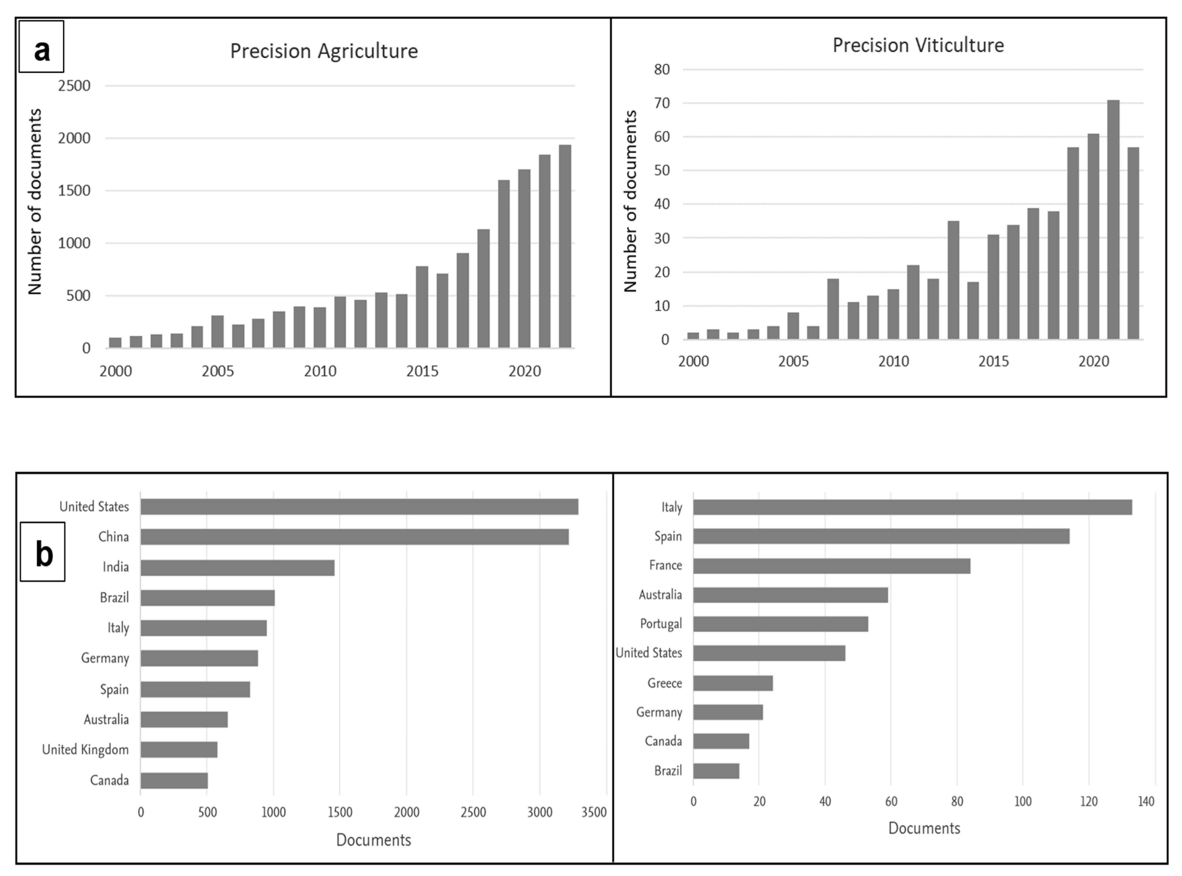
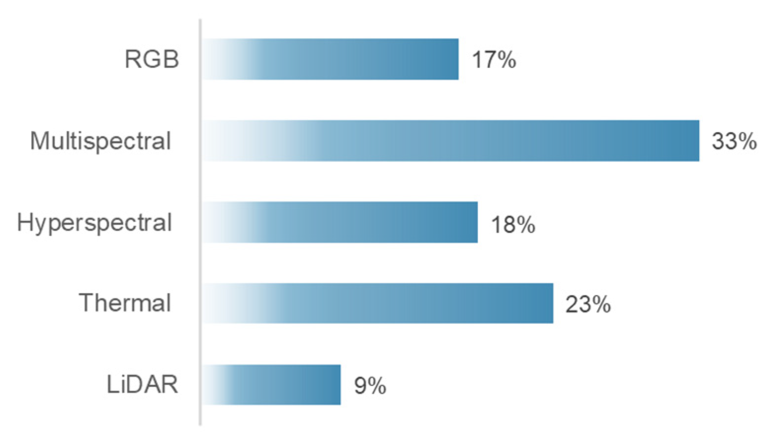
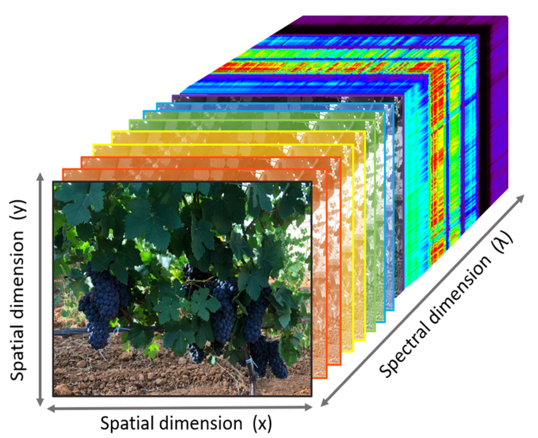
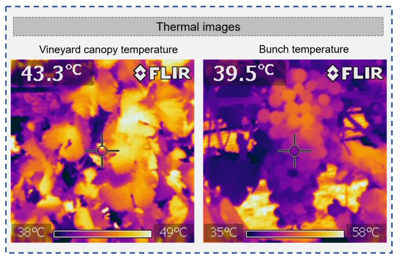
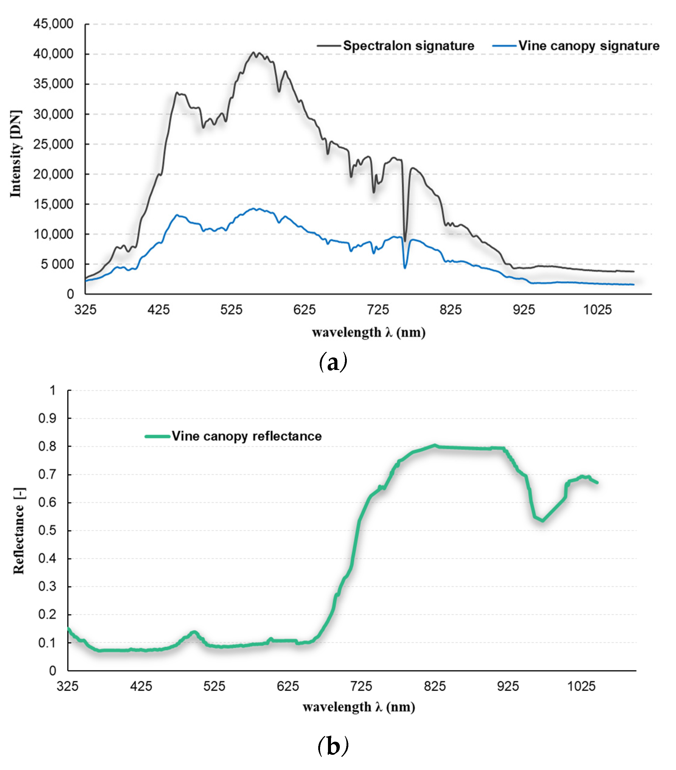
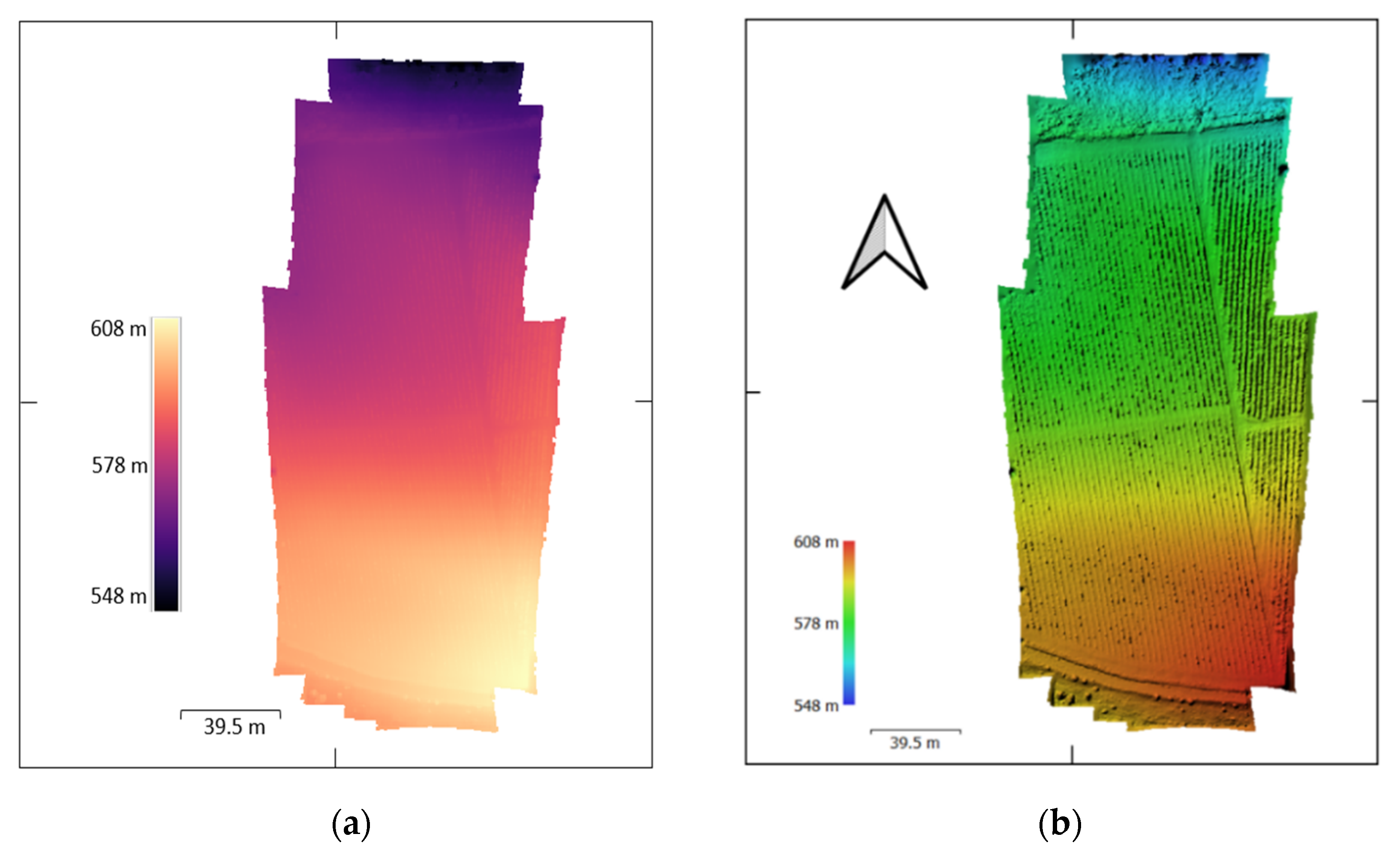
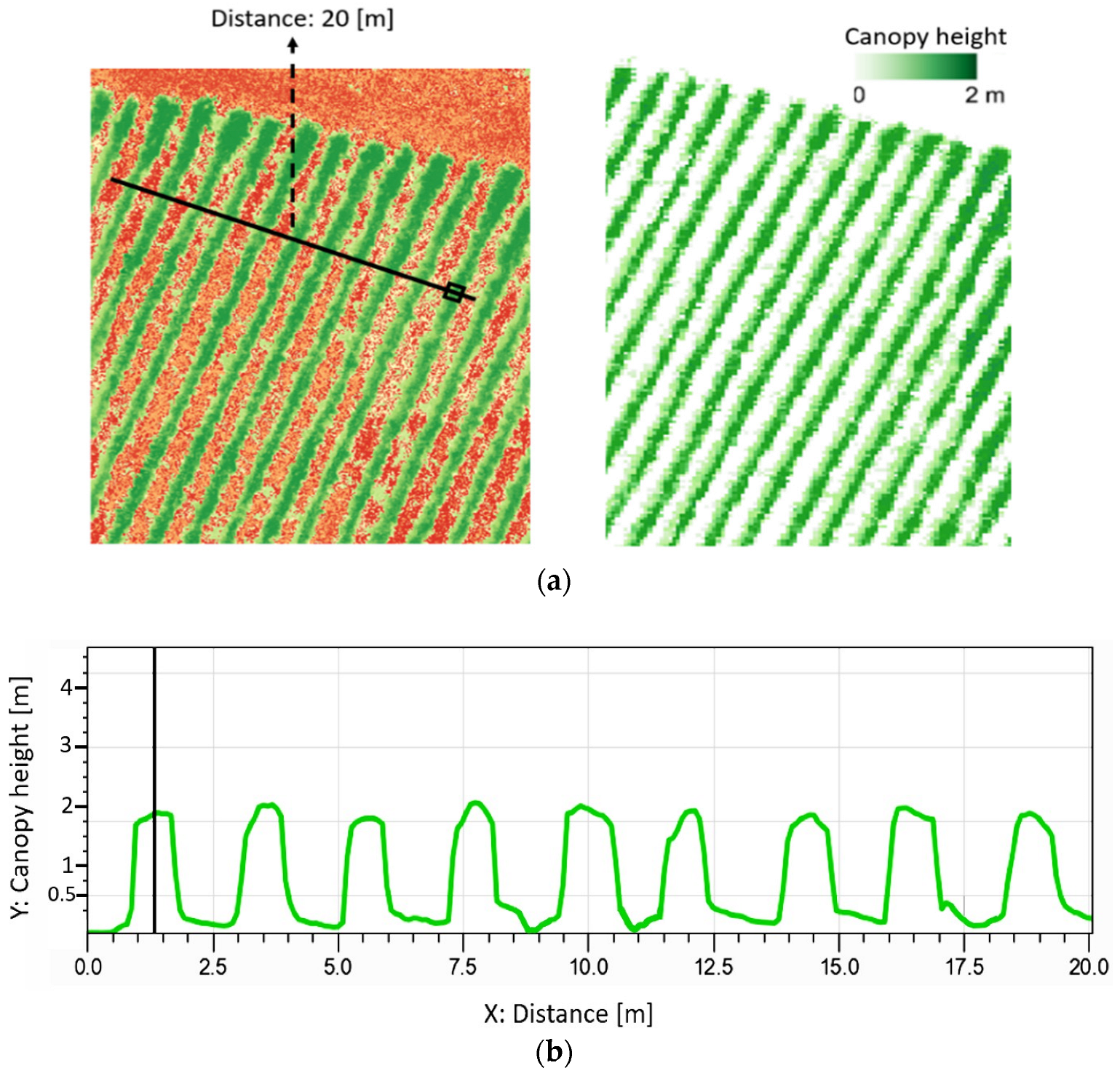
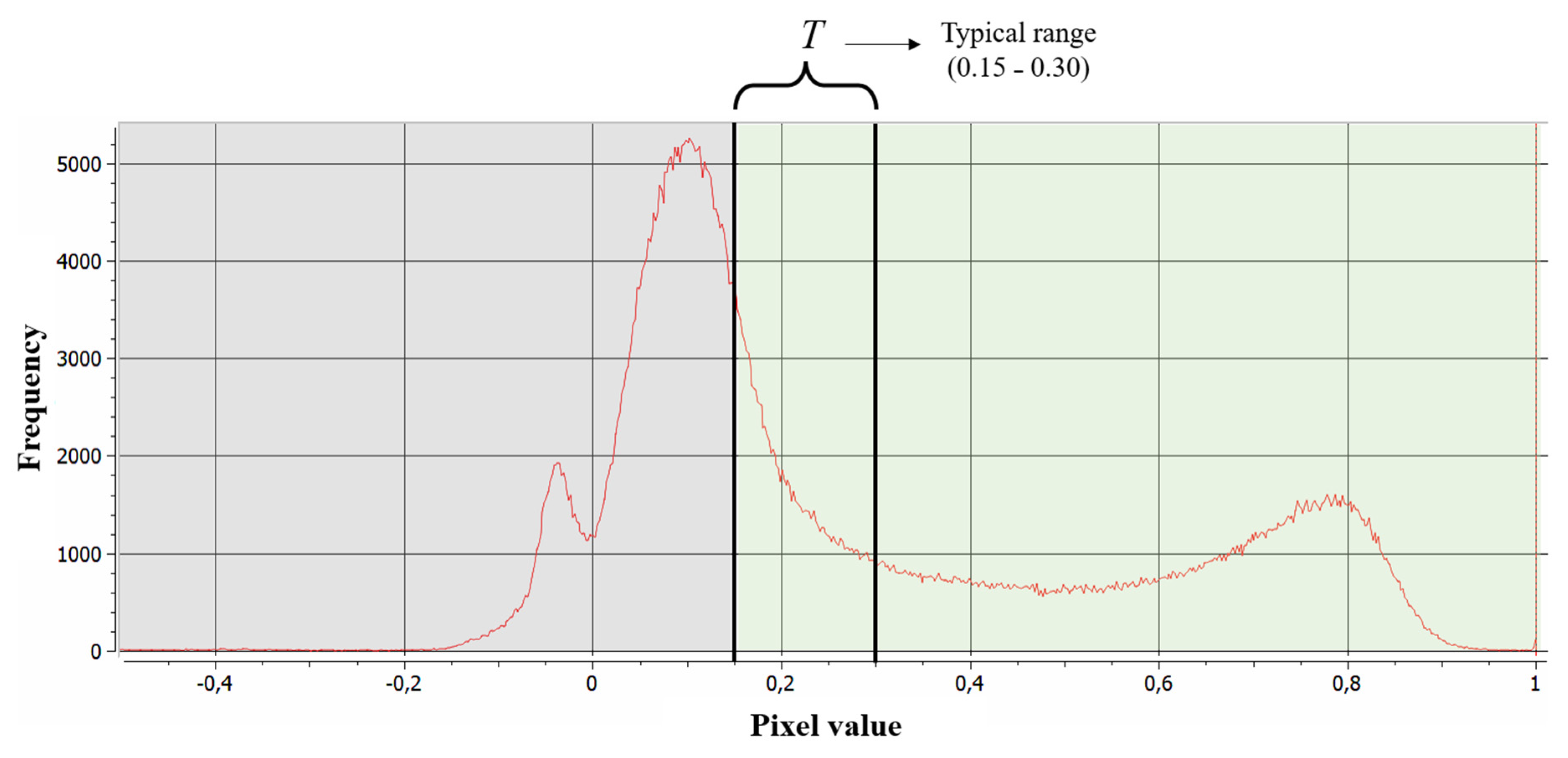
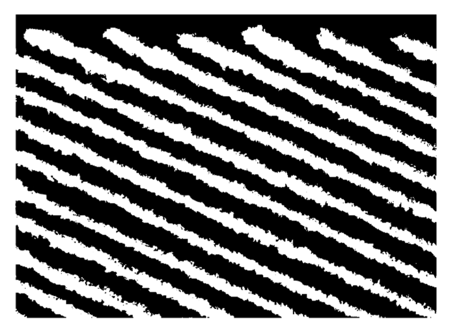
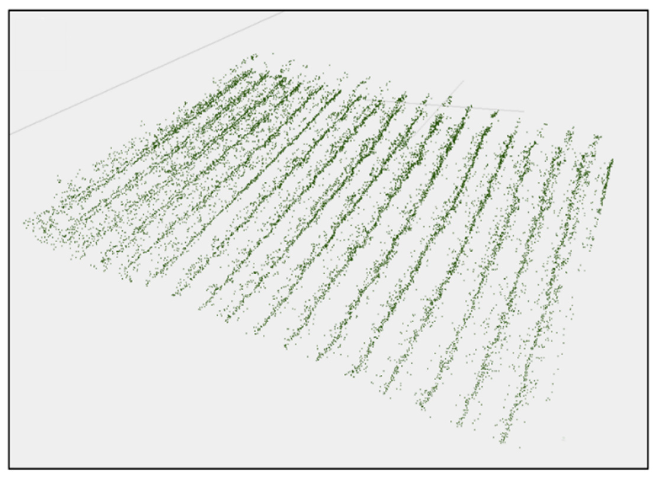
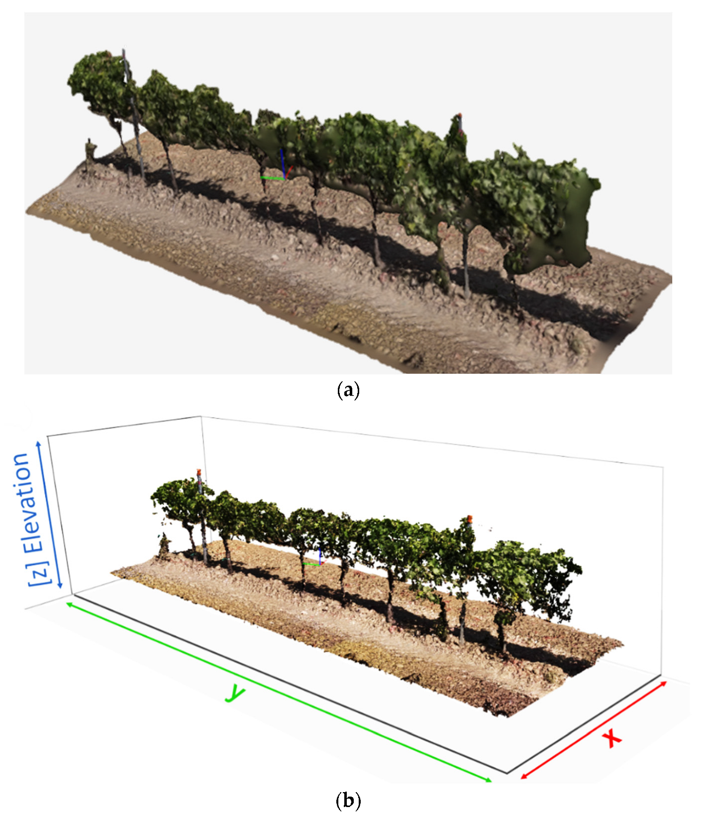
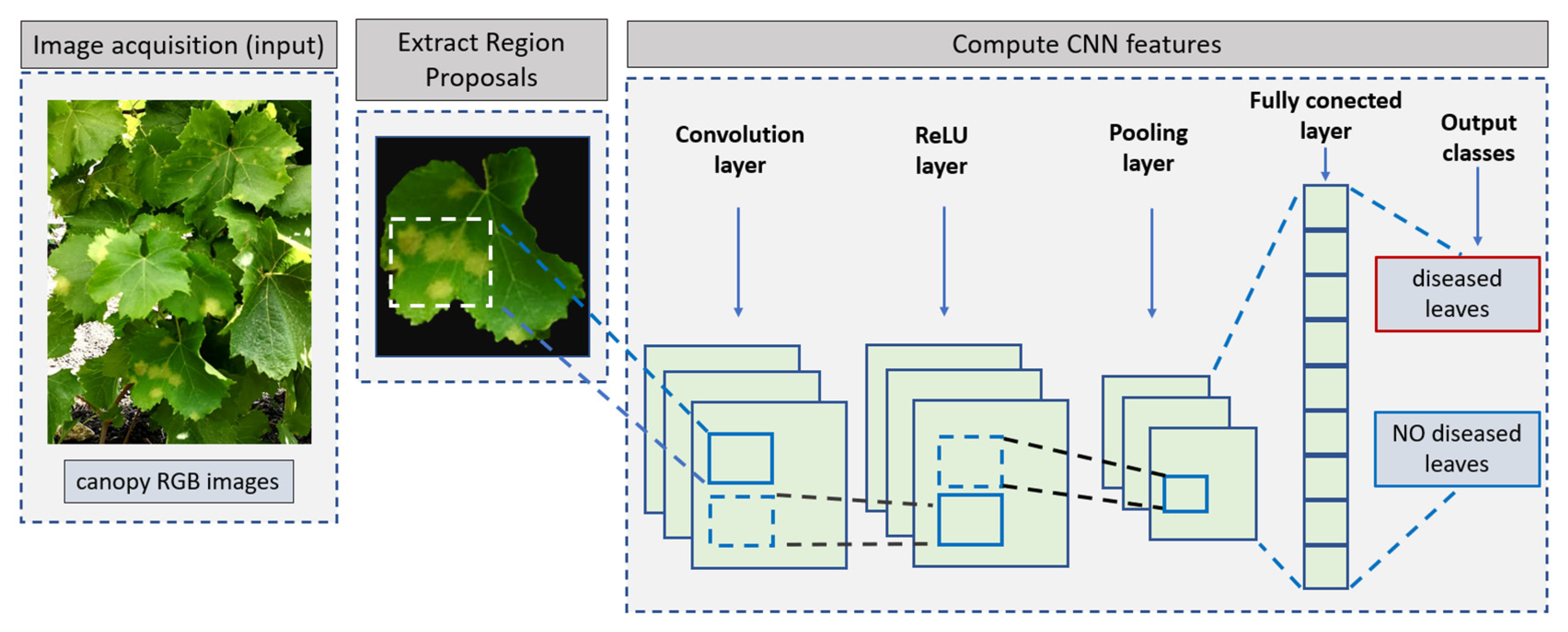
Table 1.
Representation of satellites used for viticulture surveys. Subscript (1) indicates the GSD for PAN bands, while subscript (2) indicates the GSD for Multispectral bands.
Table 1.
Representation of satellites used for viticulture surveys. Subscript (1) indicates the GSD for PAN bands, while subscript (2) indicates the GSD for Multispectral bands.
| Satellite | Temporal Cover Age | Spectral Bands | Ground Sample Distance (GSD) | Global Revisit Time |
|---|---|---|---|---|
| RapidEye AG | 1996–2020 | VIS-NIR | 6.5 m | 5.5 days |
| IKONOS | 1999–2015 | PAN-VIS-NIR | 0.8 m (1)–3.6 m (2) | 3 days MS 12 days PAN |
| MODIS | 1999–present | VIS-NIR | 250–500 m | 2 days |
| ASTER | 1999–present | VIS-NIR | 15 m | 4–16 days |
| Quickbird | 2001–2015 | PAN-VIS-NIR | 0.6 m (1)–2.5 m (2) | 3 days |
| TerraSAR-X | 2007–present | X-band SAR | 3 m | 3 days |
| WorldView-2 | 2009–present | PAN-VIS-NIR | 0.46 m (1) –1.84 m (2) | 1 day |
| Planet | 2009–present | VIS-NIR | 3.7 m | 1 day |
| WorldView-3 | 2014–present | PAN-VIS-NIR | 0.31 m (1)–1.24 m (2) | 1 day |
| Sentinel-2 | 2015–present | VIS-NIR | 10 m | 5 days |
Table 2.
The most calculated vegetation indices (VI) for viticulture surveys.
| Vegetation Index (VI) | Equations | ID | Author of Index |
|---|---|---|---|
| Excess Green (ExG) | 1 | [191] | |
| Excess Red (ExR) | 2 | [191] | |
| Normalized Difference Vegetation Index (NDVI) | 3 | [192] | |
| Simple Ratio (SR) | 4 | [193] | |
| Green Normalized Difference Vegetation Index (GNDVI) | ( | 5 | [194] |
| Modified simple ratio (MSR) | 6 | [195] | |
| Renormalized Difference Vegetation Index (RDVI) | ( | 7 | [193] |
| Soil Adjusted Vegetation Index (SAVI) | 8 | [196] | |
| Enhanced vegetation index (EVI) | 2.5 ( | 9 | [197] |
| Normalized Difference Red-Edge Index (NDRE) | ( | 10 | [198] |
| Modified Soil Adjusted Vegetation Index (MSAVI) | 11 | [199] | |
| Optimized Soil-Adjusted Vegetation Index (OSAVI) | 12 | [200] | |
| Modified Chlorophyll Absorption in Reflectance Index (MCARI) | 13 | [201] | |
| Transformed Chlorophyll Absorption Ratio Index (TCARI) | 14 | [202] | |
| Anthocyanin (Gitelson) | 15 | [203] |
Disclaimer/Publisher’s Note: The statements, opinions and data contained in all publications are solely those of the individual author(s) and contributor(s) and not of MDPI and/or the editor(s). MDPI and/or the editor(s) disclaim responsibility for any injury to people or property resulting from any ideas, methods, instructions or products referred to in the content. |
© 2023 by the authors. Licensee MDPI, Basel, Switzerland. This article is an open access article distributed under the terms and conditions of the Creative Commons Attribution (CC BY) license (https://creativecommons.org/licenses/by/4.0/).
Share and Cite
MDPI and ACS Style
Ferro, M.V.; Catania, P. Technologies and Innovative Methods for Precision Viticulture: A Comprehensive Review. Horticulturae 2023, 9, 399. https://doi.org/10.3390/horticulturae9030399
AMA Style
Ferro MV, Catania P. Technologies and Innovative Methods for Precision Viticulture: A Comprehensive Review. Horticulturae. 2023; 9(3):399. https://doi.org/10.3390/horticulturae9030399
Chicago/Turabian StyleFerro, Massimo Vincenzo, and Pietro Catania. 2023. "Technologies and Innovative Methods for Precision Viticulture: A Comprehensive Review" Horticulturae 9, no. 3: 399. https://doi.org/10.3390/horticulturae9030399
Note that from the first issue of 2016, this journal uses article numbers instead of page numbers. See further details here.