HeLoDL: Hedgerow Localization Based on Deep Learning

Abstract

Accurate localization of hedges in 3D space is a key step in automatic pruning. However, due to the irregularity of the hedge shape, the localization accuracy based on traditional algorithms is poor. In this paper, we propose a deep learning approach based on a bird’s-eye view to overcoming this problem, which we call $HeLoDL$. Specifically, we first project the hedge point cloud top-down as a single image and, then, augment the image with morphological operations and rotation. Finally, we trained a convolutional neural network, $HeLoDL$, based on transfer learning, to regress the center axis and radius of the hedge. In addition, we propose an evaluation metric OIoU that can respond to the radius error, as well as the circle center error in an integrated way. In our test set, $HeLoDL$ achieved an accuracy of 90.44% within the error tolerance, which greatly exceeds the 61.74% of the state-of-the-art algorithm. The average OIoU of $HeLoDL$ is 92.65%; however, the average OIoU of the best conventional algorithm is 83.69%. Extensive experiments demonstrated that $HeLoDL$ shows considerable accuracy in the 3D spatial localization of irregular models.

1. Introduction

With the rise of the concept of “carbon peaking and carbon neutral”, the task of achieving green development has become the mission of the times. Regular maintenance of hedges is an important task in the green development process. However, due to the increasing number of hedges, it has become increasingly difficult to rely on manual maintenance. Recently, automated hedge trimmers have been widely used, which can greatly reduce labor costs and avoid some potential safety hazards caused by manual garden maintenance. However, for hedges, it is difficult to locate them automatically because of their extremely irregular shape. As mentioned in the AdaHC [1] proposed by Li et al., the key to automating hedge maintenance is the precise localization of its center axis and radius. The precondition for the implementation of the AdaHC method is that the camera must be above the hedge. However, at this point, it is not certain where the hedge is, so the solution is not fully automated. Therefore, the 3D localization of hedges is the key to automated trimming.

The shape of the hedges studied in this paper was mainly sphere-like hedges. The hedge point cloud is used as the initial data. Thus, the problem was transformed into a localization problem for irregular spherical shapes. The target was to obtain the central axis of the hedge, as well as the height information. Previous methods for 3D object localization [2,3,4] were based on traditional algorithms, which can show relatively good results for regular models. However, because of the irregularity of the hedge, the fitting results have more uncertainties. Therefore, the location methods based on these traditional algorithms still have a big defect.

However, Krizhevsky et al. proposed the object classification algorithm AlexNet [5] based on deep learning in the ImageNet [6] contest. As a result, the deep learning algorithm [7,8,9,10] emerged, and its detection accuracy and speed far exceeded the effect based on the traditional algorithm at that time. With the development of autonomous driving technology in recent years, some excellent point-cloud-based perception solutions have been proposed [11,12,13,14]. These solutions have inspired us greatly, although they cannot locate hedges directly.

In this paper, we propose a novel 3D hedge localization method based on deep learning. Firstly, the height H of the hedge point cloud is quickly obtained by heap sorting. Secondly, the hedgerow’s point cloud is projected onto a single-channel image with a resolution of $900\times 900$. Each pixel width corresponds to the actual distance of $0.5$ cm, and the center of the image is the centroid of the point cloud in the XOY plane. Thirdly, the two-dimensional convolution neural network was used to extract the image features. Finally, the detection head module was used to regress the hedge center axis $\left(X,Y\right)$ and radius R. Moreover, inspired by the intersection over union (IoU), we propose the intersection and union ratio between circles as one of the evaluation indexes of the prediction results, which we call the OIoU. The main contributions of this paper are as follows:

a. A method of extracting green hedge point cloud information from images is proposed. This method uses pixel information to extract point cloud information by associating pixels with point clouds.

b. A method based on deep learning is proposed for the 3D localization of hedges. Its accuracy outperforms the state-of-the-art methods by a significant margin.

c. An evaluation index, the OIoU, is proposed. Combining center distance error and radius error, this index can measure the coincidence degree between circles more effectively.

d. A data augmentation method of rotating the image around the center of the mark is proposed. This method not only greatly improves the accuracy of the model, but also accelerates the convergence of the model.

The rest of this paper is organized as follows. First, the related works are introduced in Section 2. Section 3 introduces the dataset, as well as the details of the proposed method. The experimental results are given and discussed in Section 4. Finally, we give the conclusions of this study and the future work that needs to be carried out in Section 5.

2. Related Work

To solve the problem of hedge localization in a more intuitive way, we need 3D localization of hedges. According to the recent literature, there are two main schemes that can be used to achieve 3D hedge localization: (1) a hedge localization algorithm based on conventional algorithms for circle fitting; (2) a hedge localization algorithm based on conventional algorithms for sphere fitting.

The hedge localization method based on conventional algorithms for circle fitting first uses min-heap sorting [15] to obtain the height information of the hedge. Then, the point cloud is projected top-down, after which the circle fitting [3,16,17] is performed on the planar point cloud to obtain the center axis and radius of the hedge. The $Hough$ transform was first proposed by Hough [16] and later popularized by [18] Duda and Hart. It is one of the basic methods to detect geometric shapes from images in image processing. The $Hough$ transform uses the transformation between two coordinate spaces to map a curve or line with the same shape in one space to a point in another coordinate space to form a peak, thus transforming the problem of detecting arbitrary shapes into a statistical peak problem. A $Hough$ circle detection algorithm of a cumulative array based on the voting strategy [19] was proposed by Kimme et al.. When the radius of the circle to be detected is known, the algorithm can accurately detect the circle of the corresponding size. However, if the radius is unknown, the algorithm needs to occupy more parameter space; not only is the calculation speed slow, but also the stability of the algorithm is poor, and it very easily results in false detection. Fischler and Bolles proposed random consistent sampling ($Ransac$) [3] for the first time. They used $Ransac$ to solve the location determination problem. Grbić et al. proposed an ellipse detection algorithm [20] based on $Ransac$ and the least-squares method, which has good practicability in medical image analysis and ultrasonic image segmentation. The idea of the $Ransac$ algorithm is to estimate the parameters of the mathematical model iteratively from a group of observation datasets containing “external points”. It has a certain probability to obtain a reasonable result, and the number of iterations must be increased to improve the probability. However, the hedge is not regular and spherical, as it may be raised in some places and depressed in others. Therefore, the $Ransac$-based method can be somewhat accurate, but there will always be some error. Therefore, it is an uncertain algorithm. For the same reason, the $minEnclosingCircle$ method in OpenCV [17] has a rather good fit for regular circles, but the fit for the green hedge circle contour is not as good as it could be.

The hedge localization method based on conventional algorithms for sphere fitting directly fits the input hedge point cloud to the sphere [2,3,21] to obtain the sphere center and radius of the hedge. The X and Y coordinates of the sphere center are then used to determine the central axis of the hedge. The height of the hedge is still obtained by the min-heap sorting method [15]. Schnabel et al. presented an automatic algorithm [22] to detect elementary shapes in unorganized point clouds, which was used in PCL [21]. The method is based on random sampling to detect planes, spheres, cylinders, cones, and tori. The algorithm is robust even in the presence of many outliers and a high degree of noise. In addition, the algorithm is conceptually simple and easy to implement. However, the algorithm is tuned according to the a priori knowledge of different primitive shapes and parameters. Cao et al. proposed a spherical parameter detection method [2] based on the hierarchical HT (HHT). The HHT can reduce the storage space and calculation time significantly and is robust to noises and artifacts. However, the method fails completely when the gradient of the object is weaker than its background gradient. Ogundana et al. implemented the accumulator of the sparse 3D matrix model [4]. This method has the advantages of memory saving, high computational efficiency, and good 3D feature detection ability in sphere experimental shape data fitting. The method has proven to be fast and accurate. However, the method only detects the sphere center coordinates because it requires that the radius of the sphere is known. In fact, the hedge sphere to be fit is unknown, so the method is not applicable to hedge sphere fitting. Wang et al. [23] proposed an energy-based method for the automatic identification of multi-spheres, which is similar to the processing flow of $Ransac$. The main difference is that an energy-based judgment indicator is applied instead of the threshold-based indicator in $Ransac$. The results showed that the method outperforms the $Ransac$- and $Hough$-based methods in terms of accuracy and robustness. However, the experimental object of the method is its regular point cloud model, while such a regular shape hardly exists in the point cloud of hedgerows, so it is not applicable to the fitting of hedgerow spheres. Furthermore, the detection speed of the method is slow and cannot achieve a real-time processing effect.

3. Materials and Methods

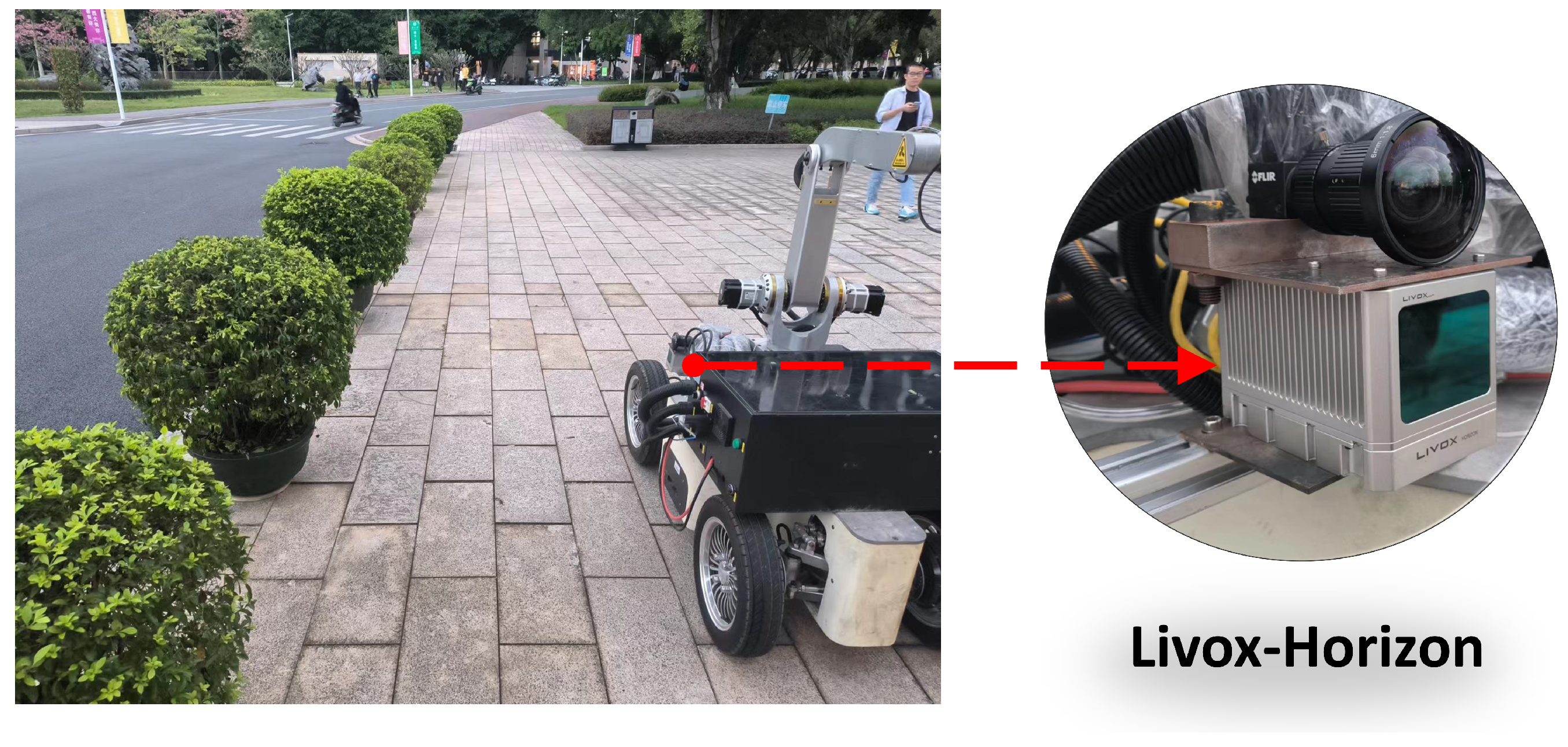
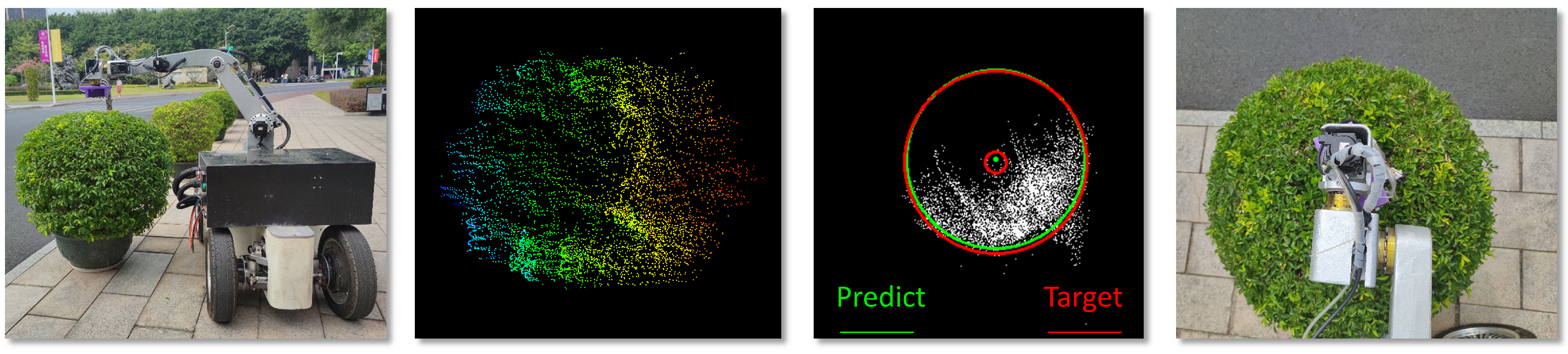
3.1. Materials

The hedge point cloud was collected with a Livox-Horizon LIDAR. Some parameters of the solid-state LIDAR Livox-Horizon are as follows. The laser wavelength is 905 nm; the distance random error is (1$\sigma$@20 m) < 2 cm; the angular random error is $1\sigma <{0.05}^{\circ }$; the beam divergence is ${0.28}^{\circ }$ (vertical) $\times {0.03}^{\circ }$ (horizontal); the field of view angle is ${81.7}^{\circ }$ (horizontal) $\times {25.1}^{\circ }$ (vertical); the measuring range $(@10$ klx) is $90m@10\%$ reflectivity; the data rate is 240,000 points per second. We collected 564 green hedge point cloud data. First, we fixed the Livox-Horizon LIDAR to the side of our unmanned car, as shown in Figure 1.

In the process of collecting data, we also noticed that the reflection intensity of the point cloud was higher when the Livox-Horizon collected at a close distance, which could not normally show the shape of the hedge at this time. Therefore, in the process of data collection, we avoided this phenomenon. The closest distance between the LIDAR and hedge was about 1 m, and the farthest distance was about 5 m. We walked along a straight line at different distances from the hedgerow to the car and recorded the point cloud bag based on the Robot Operating System [24]. It is necessary to be aware that the hedge is on the side of the car and not in front of it. In addition, due to the nature of the near-dense and far-sparse hedge point clouds, different acquisition distances were used to enrich the diversity of the samples and, thus, improve the robustness of the network model. We sampled the data at intervals of 10 frames. The traveling speed of the acquisition equipment was about 1 m/s, and the overlap rate of point clouds between two adjacent sampling points was between 27% and 79%. In addition, the distance between each hedge was about 1 m. Because the collection equipment was moving forward, we could extract the point cloud of the same hedge at different angles, which can also enrich the diversity of the data. Then, using the point cloud processing software CloudCompare [25], a total of 564 hedge point clouds were extracted from all frames of the data. In addition, we performed the dilation and erosion operations on the data, which were used to increase the amount of points in the dataset. We also rotated the data to expand the dataset. The workflow followed in the process of the morphological operation and image rotation will be described in detail in Section 3.3.3 and Section 3.3.4. The dataset is divided as shown in

Table 1. The details of the dataset.

Dataset	Hedge’s Point Cloud	Projected Image	Augmented Data
Training set	334	334	12,024
Validation set	115	115	4140
Testing set	115	115	\

.

Then, we circled the maximum outer circle of the point cloud contour in the original image without morphological operations based on the Labelme [26] software as the annotation information of the image. We invited three skilled and experienced gardeners to participate in our image annotation. Skilled gardeners were asked because it is more informative to use their experience as a criterion to determine the circles to be trimmed. Then, two rules were established that need to be followed during the annotation process. First, the annotated circle should coincide with the point cloud outline of the hedge as much as possible. Second, if it was difficult to identify the circles represented by the point cloud wheel outline, the labeling should strictly follow the actual boundary of the hedge. After the three gardeners were labeled separately, the average of the three labeling results was obtained and used as the final labeling result. Thus, the mean value of the measurements was the final labeling result for each sample. Finally, each labeled circle consisted of two key points, one of which was the center of the circle and the other a point on the boundary of the circle. The distance between these two key points was the radius. Additionally, we specifically counted the circle center coordinates X, circle center coordinates Y, and radius R for each sample and converted these coordinates to values in the LIDAR coordinate system to find their standard deviations. The respective maximum values of the three standard deviations were 0.0208, 0.0221, and 0.0242, respectively. On the other hand, the height information of the hedge was measured by three experienced gardeners using the CloudCompare software, based on the original point cloud of the hedge. As before, we averaged the measurements of the three people and used them as height annotation information for the hedge point cloud.

3.2. Problem Formulation

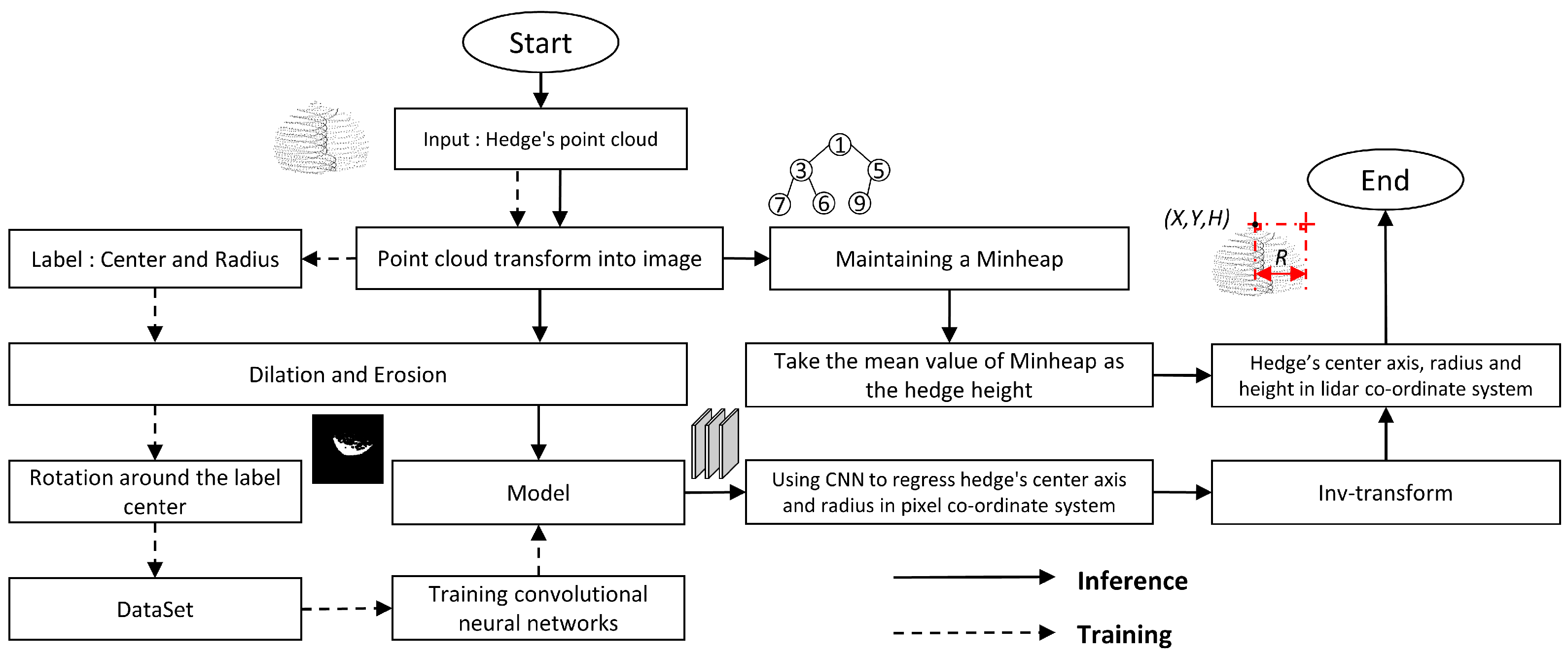
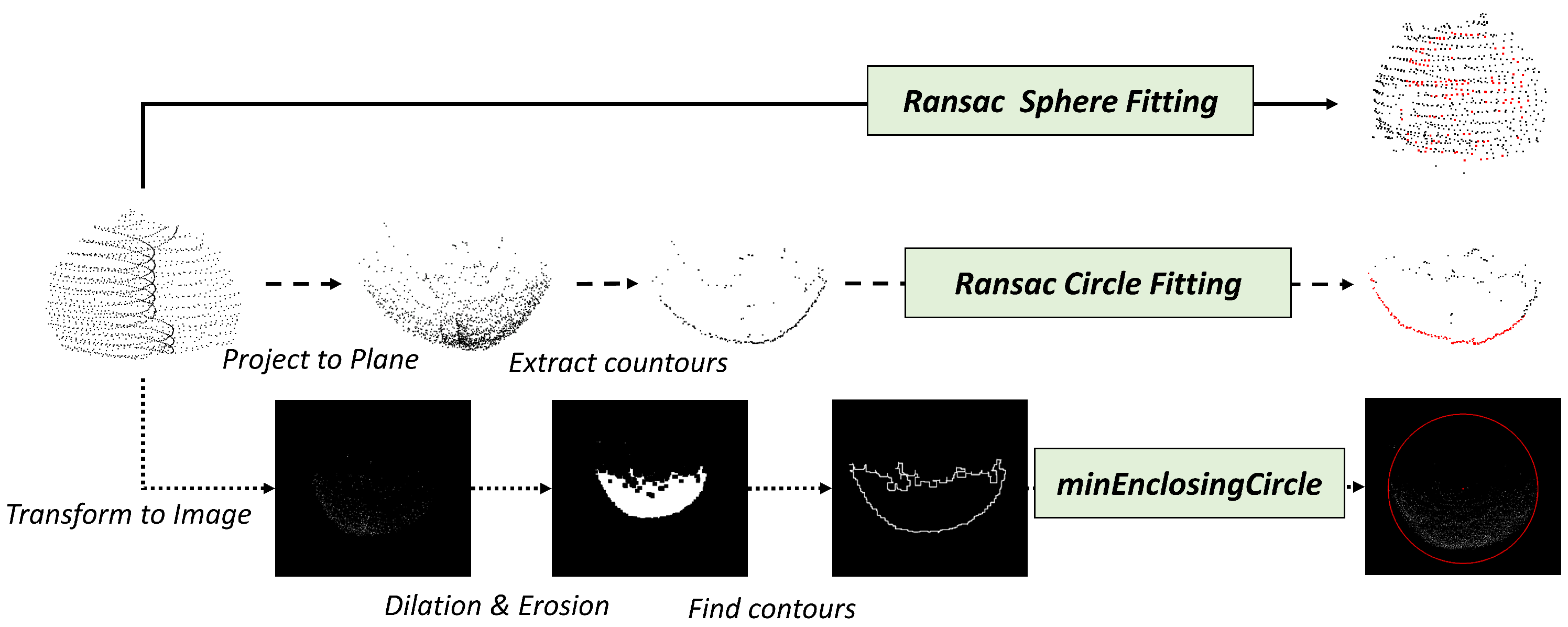
In the operation of the automatic trimmer, the trimmer needs to be placed directly above the hedge, so the height information at the top of the hedge and the center axis of the hedge need to be known. In addition, the hedge radius was used to determine whether the hedge needs to be trimmed because there are always some hedges that are not well grown and are too small to be trimmed. It is worth mentioning that if the LIDAR is mounted low, there may be a lack of information on the top of the hedge. This problem can be improved in two ways. Firstly, the hedge was localized at different measurement distances l. The localization results were converted to the world coordinate system, and their average value was taken as the final localization result. The other is to adjust the height h of the LIDAR mounting position to ensure that the LIDAR can detect the top of the hedge. Both l and h in the above two options need to be calibrated to the actual scene. In our experiments, the LIDAR was installed at a height of 0.8 m, and the data collected ranged from 1 m to 5 m.

In this paper, given a point cloud $\mathcal{X}\in {\mathbb{R}}^{N\times 3}$ of a hedgerow, we aimed to obtain its center axis $\left(X,Y\right)$, radius R, and height H. The center axis $\left(X,Y\right)$ and height H were used to adjust the position of the trimming tool, and the radius R was used to determine the working range of the trimming tool. The overall framework of our approach is shown in Figure 2.

3.3. Pipeline of $HeLoDL$

The overall framework of our approach is shown in Figure 2, and the main steps are shown as follows:

(0) Input: Hedge’s point cloud.

(1) Extract hedge’s height: We used min-heap sorting to extract the hedge’s height according to the Z coordinate of the point cloud.

(2) Transform the point cloud information into image information: The X coordinate and Y coordinate of all point clouds were averaged, respectively, to obtain $\overline{X}$ and $\overline{Y}$. Then, the center pixel of the image corresponds to $(\overline{X},\overline{Y})$. At the same time, the actual distance $0.5$ cm is represented by each pixel width. Then, all point clouds within $2.25$ m from front to back and left to right were projected onto the image relative to $(\overline{X},\overline{Y})$. Finally, if the point in the point cloud was projected onto a pixel, the pixel value was set to 255; otherwise, the pixel value was set to 0. Then, a binary image with a resolution of $900\times 900$ was obtained.

(3) Morphological operation: The aerial view obtained by Step 2 was dilated and eroded by the image morphology to fill the gap in the image and filter out some noise points on the edge.

(4) Rotation operation: All the images obtained from Step 3 were rotated around the center of the marked circle and then used as the dataset of the experiment.

(5) Using the CNN to regress center axis $(u,v)$ and radius r: The image obtained in the fourth step was directly used as the input to the convolutional neural network. The features of the image were first extracted by the mainstream backbone, and then, the size and channels of the feature layers were further compressed by the convolution neural network. The final output feature sizes of the network were $2\times 1\times 1$ and $1\times 1\times 1$, which represent the center axis $\left(u,v\right)$ and radius r of the hedge, respectively.

(6) Coordinate transformation: Transform u, v, and r in the pixel coordinate system to the corresponding point cloud coordinate system to obtain X, Y, and R.

(7) Output: Center axis $\left(X,Y\right)$, height H, and radius R.

In the later subsection, we provided a detailed description of the main content of the above process.

3.3.1. Extract the Height Information of Hedge

This paper focused on how to obtain localization information for a given hedge point cloud. The point cloud data preprocessing, however, involves our earlier work. The earlier work mainly included joint LIDAR and camera calibration, hedge detection, frustum generation, ground filtering, direct-pass filtering, and point cloud clustering. Therefore, the work on point cloud data pre-processing was performed in the early stage and is not shown in the paper. Therefore, we can assume that the hedge point cloud objects in this paper are already the point cloud after filtering out the outliers. For the extraction of hedge height, we sorted the point cloud Z value from large to small, and the average value of the point cloud with the first $5\%$ of the Z value represents the actual height of the hedge. We used the small root heap sorting algorithm to set the data capacity of the heap to $5\%$ of the number of all point clouds, pressed the Z value of $5\%$ of the point cloud into the heap, traversed the remaining $95\%$ of the point cloud, and compared the Z value with the value of the top element of the heap. If it is greater than the top element of the heap, remove the top element of the heap, and put it into the heap according to the sorting rule of the small root heap; otherwise, skip the point. It is important to note that the value of 5% is based on the data we currently used for testing. This parameter was not fixed. It was obtained by calibrating the number of point clouds for different sizes of hedges and LIDAR according to the actual situation.

$$\left\{\begin{array}{c}H=\frac{1}{n}{\sum }_{i=k}^n{Z}_i\\ k=0.95n\end{array}\right.$$

(1)

where H represents the height of the top of the hedge in the LIDAR coordinate system, n represents the number of points in the point cloud, and k represents $95\%$ times the total number of points. The time complexity of the algorithm is $O\left(nlogm\right)$, and m represents $5\%$ of the number of point clouds.

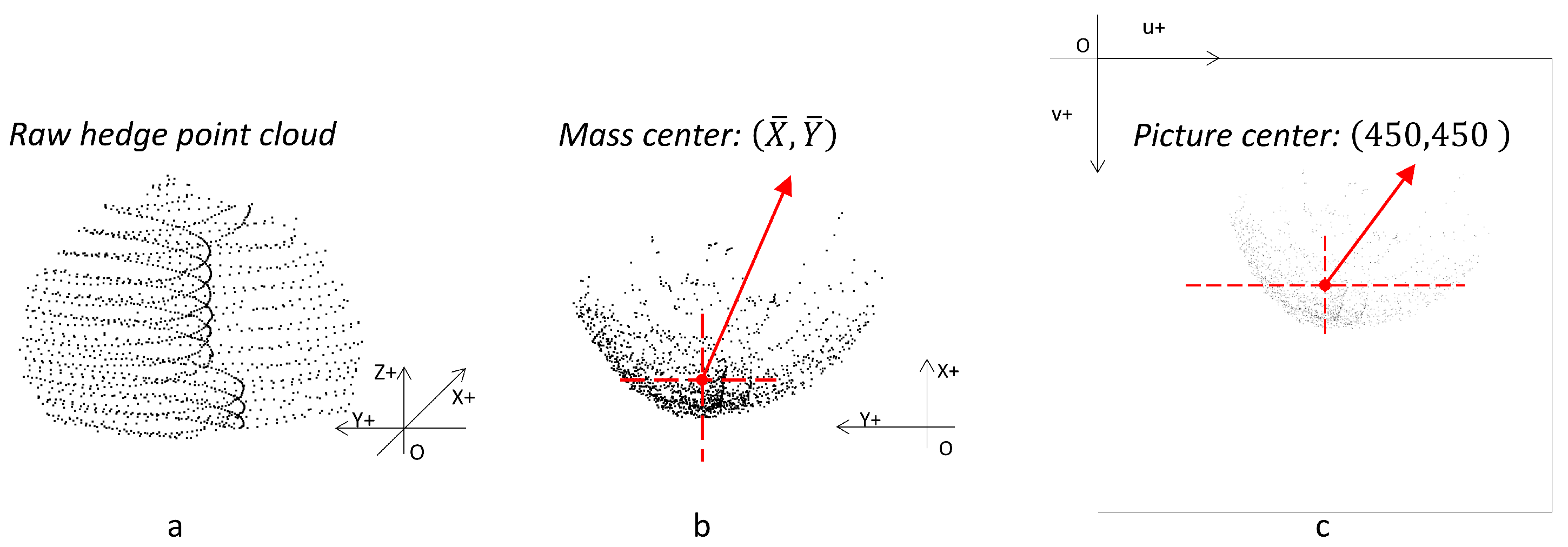
3.3.2. Transform Point Cloud Information into Image Information

After the height of the hedge was obtained, we transformed the point cloud information into image information. The process of transformation is shown in Figure 3. Firstly, these point clouds were projected on the plane to obtain point clouds in the XOY plane in the LIDAR coordinate system. Secondly, the average values of the X axis and Y axis of the plane point cloud in the LIDAR coordinate system $\overline{X}$ and $\overline{Y}$ were obtained, respectively, and then, a pixel matrix with a $900\times 900$ resolution was created. This corresponds to the $\left(\overline{X},\overline{Y}\right)$ coordinates of the plane point cloud to the pixel at $\left(450,450\right)$ in the pixel coordinates. The positive direction of the X axis in the LIDAR coordinate system is inthe negative direction of the v axis in the pixel coordinate system, and the positive direction of the Y axis in the LIDAR coordinate system is inthe negative direction of the u axis in the pixel coordinate system. Then, a binary image containing the actual location information of the point cloud was generated. The correspondence between the coordinates of the planar point cloud in the LIDAR coordinate system and the pixel coordinates is shown as follows:

$$\left\{\begin{array}{cc}{u}_0=\frac{\overline{Y}-Y}{0.5}\ast 100+450& \overline{Y}-2.25\le Y\le \overline{Y}+2.25\\ v_0=\frac{\overline{X}-X}{0.5}\ast 100+450& \overline{X}-2.25\le X\le \overline{X}+2.25\end{array}\right.$$

(2)

where ($u_0$,$v_0$) represents the coordinates of each pixel on the generated image. It should be noted that the range of 2.25 m from the center of mass was chosen based on the actual situation. The first thing was to make sure that the point cloud of the hedge did not exceed this range. Secondly, it was considered that no hedge point cloud would be outside this boundary when we rotate the image around the center of the label.

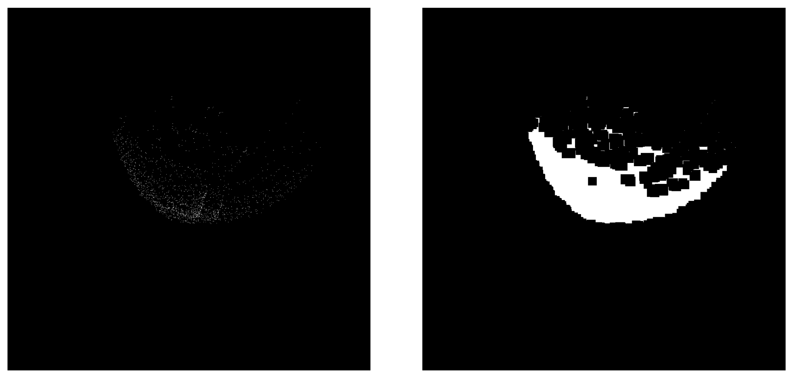
3.3.3. Morphological Operation

There is a problem with the images obtained from the above steps. Due to the sparsity of the point cloud, the percentage of pixels of the point cloud on the image was very small, and the distribution was relatively discrete. Intuitively, the point clouds occupied a small number of pixels after projection onto the image. From the statistics in our dataset, the largest cluster of point clouds had 8000 points, and the resolution of the image was 900 × 900. The number of pixels in the point cloud after projection was less than 1% of the pixels on the image, so we believe that it is a relatively small percentage. Therefore, we performed morphological operations on the image to make its features more obvious and to filter out some noise at the same time. There are corrosion and dilation operations in image morphological processing. The corrosion operation takes the minimum value in a neighborhood of each location as the output pixel value of that location, while the dilation operation is on the contrary. Therefore, for the sparse point cloud projection map, we used the operation of dilating and then eroding to increase its features and filter out the excess noise, as shown in Figure 4.

The principle to dilate the original image is as follows:

$$A\oplus B=\left\{{(x,y)|\left(B\right)}_{xy}\cap A\ne \varphi \right\}$$

(3)

where $A\oplus B$ means to dilate Image A with Structural Element B. In the above formula, ${\left(B\right)}_{x,y}$ means that the origin of the structural element B is translated to $\left(x,y\right)$. If the element in B intersecting with A is not empty, then the pixel value at $\left(x,y\right)$ is 0; otherwise, it is 255.

The principle to erode the original image is as follows:

$$A\ominus B=\left\{{(x,y)|\left(B\right)}_{xy}\subseteq A\right\}$$

(4)

where $A\ominus B$ means to erode Image A with Structural Element B. If all the elements in B belong to A, then the pixel value at $\left(x,y\right)$ is 255; otherwise, it is 0.

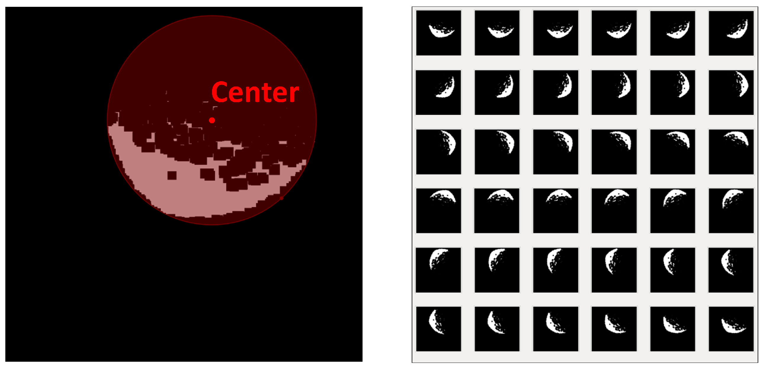
3.3.4. Rotation Operation

After the previous steps, we obtained the image from point cloud projection and processed by dilation and erosion, but the images we input were only irregular figures, similar to a crescent moon. Because the point cloud of the hedge scanned by LIDAR is only single-sided and the orientation of the point cloud shape on the image is also single after conversion to a picture, we conjectured that, by the rotation of the image, the neural network can learn more features of the circle to achieve better prediction. Although the input data are only one-sided in practice, this does not impact enhancing the learning of circular features by rotating the initial dataset. Additionally, since the center of rotation is the center of the labeled circle, it does not change the central axis of the hedge point cloud, nor the radius, even after rotation. Therefore, we rotated the point cloud image around the center point of our label according to a series of angles. The corresponding relationship of pixel coordinates before and after image rotation is shown in the following formula:

$$\left[\begin{array}{c}{u}_1\\ v_1\end{array}\right]=\left[\begin{array}{cc}cos\theta & -sin\theta \\ sin\theta & cos\theta \end{array}\right]\left[\begin{array}{c}{u}_0-Center\left[0\right]\\ v_0-Center\left[1\right]\end{array}\right]+\left[\begin{array}{c}Center\left[0\right]\\ Center\left[1\right]\end{array}\right]$$

(5)

where $Center$ represents the center of the labeled circle, $\theta$ represents the angle of counterclockwise rotation, and $\left(u_1,v_1\right)$ represents the coordinates of each pixel after rotation.

The details of the rotation and the working criteria can be described as follows. First, the center of rotation is the center of the labeled circle. Second, the object of rotation is the pixel with the pixel value of 255 in the original image. Third, the rotation angle interval is 10°. The purpose of the third step is to train the neural network to learn richer features, so the rotation angle interval was set relatively small. The image data after rotation is shown in Figure 5.

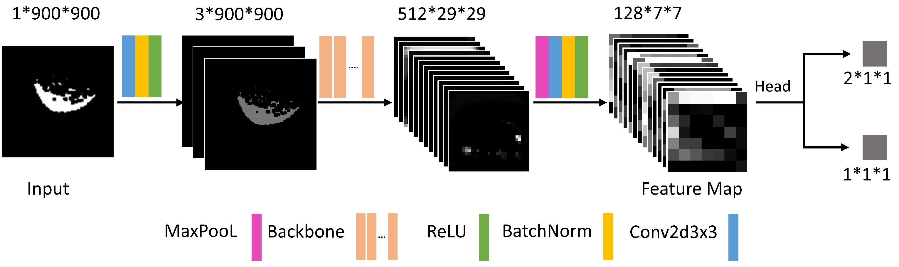
3.3.5. Using CNN to Regress Center Axis (u, v) and Radius r

As shown in Figure 6, the input of the neural network is a single-channel image with a resolution of $900\times 900$, while the input images of the more popular backbone are three-channel RGB images. To be able to use transfer learning to accelerate the convergence of the network model, we first expanded the image to three channels by a layer of $3\times 3$ convolution. At this point, the backbone and its pre-trained model, which are the mainstream in academia, were used to extract the features of the images. The output of the backbone is the feature layer of $512\times 29\times 29$, and the visualization of some of its channels is shown in Figure 7. The maximum pool and convolution layer were used to further compress the feature layers, and the number and size of channels were compressed to the size of $128\times 7\times 7$.

The head part of the model is mainly divided into two branches, namely $C{T}_{Head}$ and $R_{Head}$. In order to improve the overall performance of the network, we added batch normalization [27] and ReLU activation functions [28] in each layer. Among them, the output of $C{T}_{Head}$ is a $1\times 1$-sized feature layer of two channels, and the two channels represent the X value and Y value of the center axis of the hedge, respectively. The output of $R_{Head}$ is a $1\times 1$-sized feature layer of a single channel, which was used to represent the radius R of the hedge. The structure of the head module is shown in Figure 8.

Since there is only one hedge to be fit in each image, no classification operation was performed in our scheme. Instead, the radius R and the center axis $\left(X,Y\right)$ of the hedge to be fitted were regressed directly, which is a typical regression problem. It is inevitable that there will be some noises after the point cloud is projected to the image, and the L1 loss function is robust against the outliers in the data, so we used the L1 loss function to measure the prediction of the model.

$$Loss={\lambda }_{CT}\frac{1}{n}\sum _{i=1}^n\left(\right|u_i-\widehat{u_i}|+|v-\widehat{v_i}\left|\right)+{\lambda }_R\frac{1}{n}\sum _{i=1}^n\left(\right|r_i-\widehat{r_i}\left|\right)$$

(6)

where $\left(\widehat{u_i},\widehat{v_i}\right)$ denotes the coordinates of the circle center of the i-th labeled circle in the pixel coordinate system and $\widehat{r_i}$ is the radius of the labeled circle; $\left(u_i,v_i\right)$ denotes the coordinates of the circle center of the i-th predicted circle in the pixel coordinate system, and $r_i$ is the radius of the predicted circle. ${\lambda }_{CT}$ is the weight of the center axis error, and ${\lambda }_R$ is the weight of the radius prediction error. As the trimming radius of our trimming tool was already determined, the accuracy of the central axis of the hedge was more important than the accuracy of the radius. Therefore, we set ${\lambda }_{CT}$ to 1 and ${\lambda }_R$ to 0.5 as a way to make the training process more focused on the task for central axis prediction.

3.3.6. Training and Inference

After we transformed the point cloud into a picture with actual distance information, we obtained a single-channel image with a resolution of $900\times 900$. We used the Adam optimizer to adjust the parameters of the model. The initial learning rate of the optimizer was set to 0.01, and the learning rate was adjusted dynamically according to the change of the loss function during the training process. In addition, we used the backbone network of $ResNet$ [29] and $ShuffleNet$ [30], respectively; meanwhile, we used transfer learning in the training process. At the initial stage of training, we first froze the weight parameters of the backbone network to prevent them from being modified prematurely. Later in the training process, we unfroze the weight parameters of the backbone network and trained them together with the whole convolutional neural network.

The inference process is different from the training process, and the rotation operation is dropped in inference. The neural network directly regresses the pixel coordinates of the center axis of the hedge point cloud $(u,v)$ and the pixel radius r. Using the formula 7, we can transform the pixel coordinate center point $\left(u,v\right)$ to the center axis $\left(X,Y\right)$ in the LIDAR coordinate system; at the same time, the pixel radius r is transformed to the radius R in the LIDAR coordinate system.

$$\left\{\begin{array}{c}R=\frac{r\ast 0.5}{100}\\ X_{CT}=\overline{X}-0.5\ast \frac{v-450}{100}\\ Y_{CT}=\overline{Y}-0.5\ast \frac{u-450}{100}\end{array}\right.$$

(7)

4. Results

The convolutional neural network was trained on a server equipped with an NVIDIA TITAN RTX GPU with 24GB of memory. The inference process of the $HeLoDL$ model and the various comparison methods were performed on a Lenovo laptop with an AMD R7 5800H CPU, 16GB RAM, and an Nvidia RTX 3060 GPU with 6GB of memory.

4.1. Evaluation Index

4.1.1. Evaluation Index Related to Center Axis and Radius

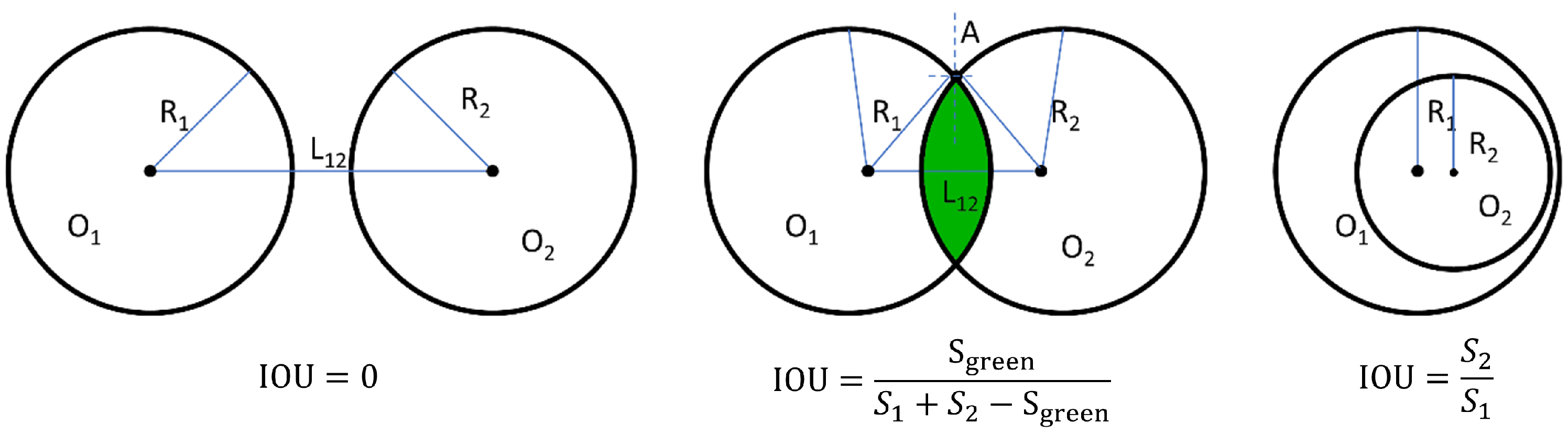
To fairly evaluate the performance of different algorithms, we considered the accuracy of the position of the center axis of the hedge $\left(X,Y\right)$ and the radius R, respectively. In our evaluation index, we stipulated that the offset of the center axis of the hedge cannot exceed 5 cm, which is a rigid index. Since each pixel grid represents the actual distance of $0.5$ cm, the distance between the location of our predicted center axis and the labeled center axis cannot exceed 10 pixels. Then, the evaluation index of circle center accuracy $C{T}_{ACC}$ is defined as follows:

$$f\left(i\right)=\left\{\begin{array}{cc}1& if\sqrt{{\left(u_i-\widehat{u_i}\right)}^2+{\left(v_i-\widehat{v_i}\right)}^2}\le 10\\ 0& otherwise\end{array}\right.$$

(8)

$$C{T}_{ACC}=\frac{1}{n}\sum _{i=1}^{n}f\left(i\right)$$

(9)

$C{T}_{ACC}$ cannot specifically express the accuracy of the algorithm. Therefore, we designed two other indicators, the average error of the radius $R_{ERR}$ and the center distance error $C{T}_{ERR}$, to represent the error of the algorithm in the center point and radius, respectively, which are defined as follows:

$$R_{ERR}=\frac{1}{n}\sum _{i=1}^n\left(|r_i-\widehat{r_i}|\right)$$

(10)

$$C{T}_{ERR}=\frac{1}{n}\sum _{i=1}^n\sqrt{{\left(u_i-\widehat{u_i}\right)}^2+{\left(v_i-\widehat{v_i}\right)}^2}$$

(11)

4.1.2. OIoU

For a single prediction circle, the distance error $C{T}_{ERR}$ of the center of the circle can effectively evaluate the accuracy of the center prediction, while the radius error $R_{EER}$ of the circle can effectively evaluate the accuracy of the radius prediction. However, the center error $C{T}_{ERR}$ and radius error $R_{EER}$ cannot directly reflect the degree of overlap of the two circles. Inspired by the classical IoU, we propose the OIoU. As shown in Figure 9, the OIoU is the ratio of the area of the intersection of two circles to the union of the areas of two circles. The OIoU can intuitively reflect the coincidence of the predicted circle with the ground truth circle, which is defined as follows:

$$OIoU=\frac{Intersection}{Union}$$

(12)

if $R_1+R_2<L_{12}$,

$$Intersection=0,Union=\pi \left(R_1^2+R_2^2\right)$$

(13)

if $R_1\ge R_2+L_{12}$,

$$Intersection=\pi R_2^2,Union=\pi R_1^2$$

(14)

if $R_2\ge R_1+L_{12}$,

$$Intersection=\pi R_1^2,Union=\pi R_2^2$$

(15)

other cases,

$$\begin{array}{c}Intersection={\theta }_{O1}{R_1}^2+{\theta }_{O2}{R_2}^2-R_1{L}_{12}sin\angle A{O}_1{O}_2-R_2{L}_{12}sin\angle A{O}_2{O}_1\\ Union=\pi \left({R_1}^2+{R_2}^2\right)-Intersection\end{array}$$

(16)

where ${\theta }_{O1}=arccos\left(\frac{{L_{12}}^2+{R_1}^2-{R_2}^2}{2L_{12}{R}_1}\right)$, ${\theta }_{O2}=arccos\left(\frac{{L_{12}}^2+{R_2}^2-{R_1}^2}{2L_{12}{R}_2}\right)$.

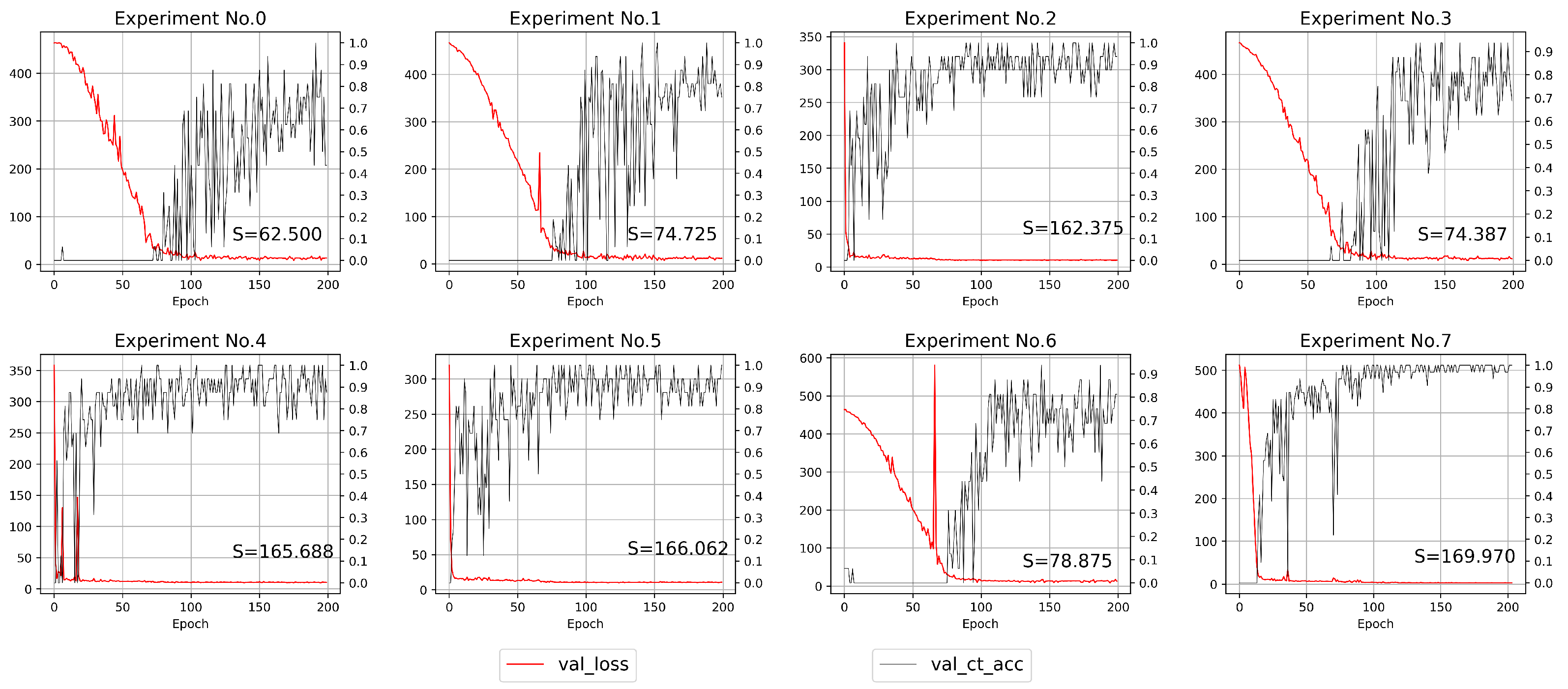
4.2. Experimental Results

We performed experiments with other baseline methods in the test set. The baseline methods to obtain the three-dimensional information of hedges through point clouds are presented in Figure 10. In the first method, the $Ransac$ sphere fitting algorithm was directly used to fit the original point cloud of the hedge. In the second method, the original green hedge point cloud was projected onto the XOY plane to obtain the plane point cloud, then the boundary points of the plane point cloud were obtained based on the normal estimation, and the circle was estimated by the $Ransac$ circle fitting algorithm based on the boundary points. In the third method, firstly, the original point cloud was projected in the top view and transformed into an image. Next, the image was dilated and eroded. Then, the contour with the most boundary points was extracted. Finally, the outer circle of the contour was extracted using the $minEnclosingCircle$ function in OpenCV.

In our method, considering the accuracy and complexity of the model, we chose a $ResNet34$-based network model and compared it with the other three solutions. It can be seen from Figure 11 that our method is obviously better than the other solutions in predicting the center and radius of the circle. As shown in

Table 2. Comparison with the state-of-the-art algorithm.

Method	${\mathit{CT}}_{\mathit{ACC}}$ (%)	${\mathit{R}}_{\mathit{ERR}}$ (cm)	${\mathit{CT}}_{\mathit{ERR}}$ (cm)	${\mathit{OIoU}}_{\mathit{mean}}$ (%)	${\mathit{Time}}_{\mathit{mean}}$ (ms)
$Ransac$ Sphere Fitting	36.522	7.091	6.935	73.775	16.603
$Ransac$ Circle Fitting	61.739	4.398	5.458	83.689	13.132
minEnclosingCircle	28.696	2.430	9.265	80.914	13.509
$HeLoDL$	90.435	1.635	2.712	92.654	12.727

, our method is significantly better than the two traditional methods in terms of center accuracy. The average center distance error in our method was $2.67$ cm, which fully meets the accuracy requirements of 5 cm. The importance of the prediction radius task is second only to the central point prediction task, and the radius error of our method was $1.61$ cm, also showing strong stability and accuracy. Of course, we can see that the time consumption of our method is very short, and we can achieve real-time processing. The OIoU metric we designed also showed a high level at the same time. The results of the predicted radius and circle center tasks can also prove the reasonableness and comprehensiveness of the OIoU.

It is also necessary to note that since the same height information acquisition scheme is used in several algorithms. Therefore, we will not compare the height information in the experimental results. Of course, the process of height information extraction is included in the inference process of each algorithm, so the time consumption of several algorithms regarding the inference process is fair.

4.3. Comparative Experiment

4.3.1. The Effect of Different Backbones

In this section, we tried different backbones, such as $ResNet$ [29] and $ShuffleNetV2$ [30]. $ResNet$ adopts the structure of the skip connection, which greatly increases the depth of the network and can extract more deep features. In addition, the $ResNet$ backbone network suppresses the problems of gradient explosion and gradient disappearance. $ShuffleNetV2$ is a lightweight backbone network in terms of speed and accuracy. In addition, in order to fit the lightweight network on embedded devices, we also tested the model based on $ShuffleNetV2$. The results are shown in

Table 3. The effect of applying different backbone networks to the model.

Backbone	${\mathit{CT}}_{\mathit{ACC}}$ (%)	${\mathit{R}}_{\mathit{ERR}}$ (cm)	${\mathit{CT}}_{\mathit{ERR}}$ (cm)	OIoU (%)	${\mathit{Infer}}_{\mathit{Time}}$ (ms)	${\mathit{Train}}_{\mathit{Time}}$ (hours)	Gflops	Parameters (millions)	Memory (M)
ResNet18	83.482	1.865	3.314	91.045	11.384	16.255	30.115	11.794	445.205
ResNet34	90.435	1.635	2.712	92.654	12.727	26.352	60.732	21.893	641.014
ResNet50	90.435	1.565	2.694	92.465	16.493	43.164	68.115	25.893	1818.297
ShuffleNet_v2_x0_5	65.224	2.573	5.559	87.364	15.103	8.261	0.792	1.543	212.841
ShuffleNet_v2_x1_0	79.132	2.114	3.691	90.062	14.844	11.943	2.583	2.455	370.992
ShuffleNet_v2_x1_5	76.527	2.452	3.687	89.674	15.213	15.697	5.132	3.684	510.53

. It can be seen that the lightweight network model has lower complexity, less computational time, and faster training speed, but the detection accuracy is not as good as that of the backbone network with a greater depth.

4.3.2. Ablation Study

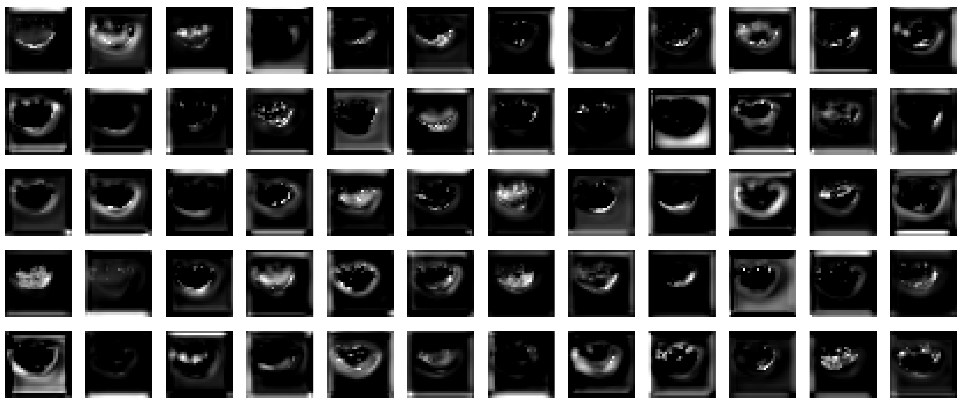
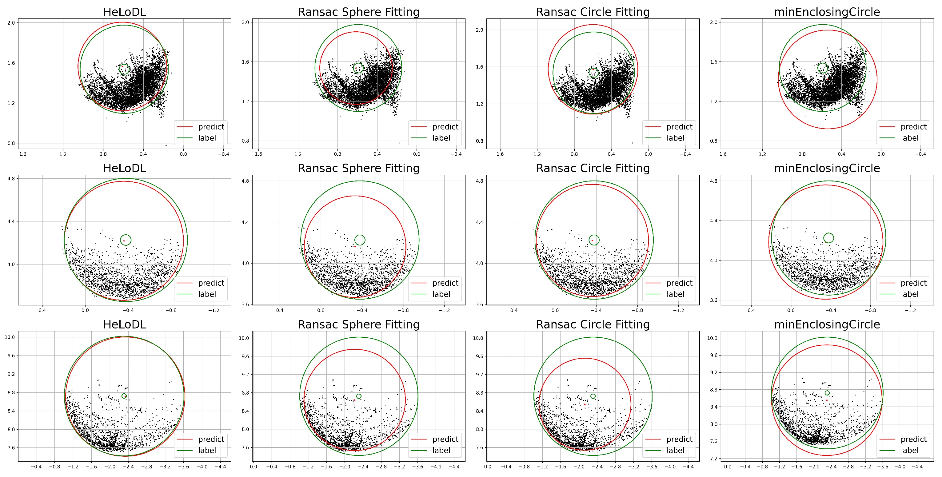
In this section, we validated the performance of different combinations of transfer learning, the rotation operation, and the morphological operation. The pre-training weight of the model is generally based on the rich dataset, but the color of the image dataset in this paper is relatively simple. Therefore, we hoped to study whether the transfer learning works well for the model proposed in this paper. At the same time, we also wanted to know the effect of image rotation and the morphological operation on the accuracy of the model. Based on this, we designed eight groups of experiments, as shown in

Table 4. The design of the ablation experiment.

Experimental Serial Number	0	1	2	3	4	5	6	7
Transfer Learning	✘	✔	✘	✘	✔	✘	✔	✔
Rotation operation	✘	✘	✔	✘	✔	✔	✘	✔
Morphological operation	✘	✘	✘	✔	✘	✔	✔	✔

. We trained the model according to the requirements of the eight groups of experiments. This experiment was based on $ResNet34$.

To analyze the influence of several operations on the model training process and model accuracy, we visualize the accuracy and loss of the model on the validation set during the training in Figure 12. In addition, in order to directly show the performance of center prediction on the validation set in each group of experiments, we used the area S of the $val\_ct\_acc$ curve and the X axis of the coordinate system, which is defined as:

$$S=\sum _{i=1}^{200}val\_ct\_acc\left(Epoc{h}_i\right)$$

(17)

where $val\_ct\_acc$ denotes the $C{T}_{ACC}$ of the model on the validation set at the time of training in each epoch. $Epoc{h}_i$ denotes the i-th time the neural network completes the forward computation and backward propagation. Moreover, in order to verify the real effects of the models in each experiment, we tested the models of each experiment using 115 sets of experimental data in the test set, respectively, and the experimental data are shown in

Table 5. Ablation study results for the test set.

Experimental Serial Number	0	1	2	3	4	5	6	7
$R_{ERR}$ (cm)	2.980	2.494	1.849	2.688	1.816	1.720	2.196	1.635
$C{T}_{ERR}$ (cm)	4.696	5.060	2.959	4.941	2.815	2.785	4.237	2.712
OIoU (%)	88.022	88.084	91.767	88.311	91.699	92.200	89.815	92.654
$C{T}_{ACC}$ (%)	71.304	72.174	86.957	74.783	87.826	88.696	76.522	90.435

.

Comparing the results of Experiments 0 and 1, 2 and 4, 3 and 6, and 5 and 7, we can observe from Table 5 that transfer learning plays a critical role in improving $C{T}_{ACC}$. Comparing the results of Experiments 0 and 2, 1 and 4, 3 and 5, and 6 and 7, in Table 5, we can estimate that the rotation operation improves the $C{T}_{ACC}$ of the model on the test set by an average of $14\%$. Furthermore, it can also be clearly seen from Figure 12 that the rotation enhancement operation of the training set not only accelerates the convergence speed of the model training, but also greatly improves the accuracy of the model. Comparing the results of Experiments 0 and 3, 1 and 6, 2 and 5, and 4 and 7, as we can see in Table 5, the morphological operation of the image also improves the $C{T}_{ACC}$.

Comparing the results of Experiments 0 and 1, 2 and 4, 3 and 6, and 5 and 7, we can observe from Table 5 that transfer learning plays a critical role in improving $C{T}_{ACC}$. Comparing the results of Experiments 0 and 2, 1 and 4, 3 and 5, and 6 and 7, in Table 5, we can estimate that the rotation operation improves the $C{T}_{ACC}$ of the model on the test set by an average of $14\%$. Furthermore, it can also be clearly seen from Figure 12 that the rotation enhancement operation of the training set not only accelerates the convergence speed of the model training, but also greatly improves the accuracy of the model. Comparing the results of Experiments 0 and 3, 1 and 6, 2 and 5, and 4 and 7, as we can see in Table 5, the morphological operation of the image also improves $C{T}_{ACC}$.

As shown in Figure 12 and Table 5, Experiment No. 7 showed the best results compared with the other groups due to the simultaneous use of transfer learning, the image rotation, and the morphological operation of the image. This strongly proves the necessity of the method of our data pre-processing and transfer learning.

4.4. Visualization

In order to demonstrate the working principle of the method in this paper more clearly, we selected a set of experiments from the actual test set data and visualize the process in Figure 13. The first three subfigures of Figure 13 show the scene acquisition, hedge point cloud extraction, and center axis localization, respectively. Finally, we used the localization results as the input for the robot arm planning control, and the last subfigure shows the final localization effect of the robot arm. It is necessary to note that the point cloud data in Figure 13 were intercepted by setting the point cloud range, because the focus of this paper was on how to obtain the accurate position information from the hedge point cloud. The experimental data in the previous section and the final robot localization position can prove that the localization accuracy of the proposed method can fully meet the practical requirements.

5. Conclusions

We investigated the 3D localization problem of hedges in a garden environment. In order to solve this problem, a novel algorithm $HeLoDL$ for the 3D localization of hedges via deep learning was proposed for the first time. We also proposed an evaluation metric, the OIoU, to evaluate the effectiveness of the localization algorithm. Additionally, we provide two networks with different model sizes so that the model can run on different devices. Extensive experiments validated that the $HeLoDL$ outperformed strong baselines by a large margin. There were some limitations in this study. First, the ground for the work should be flat. Additionally, the mounting height of the LIDAR needs to be adjusted according to the height of the hedge in the working scenario. Therefore, in order for the system to show high working performance in practical applications, the following requirements can be made for the environment. Firstly, the ground on which the device runs should be as flat as possible. Secondly, the trimmed hedges should be near the flat road surface and the hedges of different large and low heights should be arranged separately as much as possible. Additionally, the data acquisition solution of $HeLoDL$ we currently provide is still not automated enough. In the future, we will consider using the point cloud segmentation scheme [31,32] to simplify the process of generating hedge point cloud datasets to some extent.

References

1. Li, Z.; Xu, E.; Zhang, J.; Meng, Y.; Wei, J.; Dong, Z.; Wei, H. AdaHC: Adaptive Hedge Horizontal Cross-Section Center Detection Algorithm. Comput. Electron. Agric. 2022, 192, 106582. [Google Scholar]
2. Cao, M.; Ye, C.; Doessel, O.; Liu, C. Spherical parameter detection based on hierarchical Hough transform. Pattern Recognit. Lett. 2006, 27, 980–986. [Google Scholar] [CrossRef]
3. Fischler, M.A.; Bolles, R.C. Random sample consensus: A paradigm for model fitting with applications to image analysis and automated cartography. Commun. ACM 1981, 24, 381–395. [Google Scholar]
4. Ogundana, T.; Coggrave, C.R.; Burguete, R.; Huntley, J.M. Fast Hough transform for automated detection of spheres in three-dimensional point clouds. Opt. Eng. 2007, 46, 051002. [Google Scholar]
5. Krizhevsky, A.; Sutskever, I.; Hinton, G.E. Imagenet classification with deep convolutional neural networks. Commun. ACM 2017, 60, 84–90. [Google Scholar] [CrossRef]
6. Deng, J.; Dong, W.; Socher, R.; Li, L.J.; Li, K.; Li, F.F. ImageNet: A Large-Scale Hierarchical Image Database. In Proceedings of the 2009 IEEE Conference on Computer Vision and Pattern Recognition, Miami, FL, USA, 20–25 June 2009; pp. 248–255. [Google Scholar] [CrossRef]
7. Girshick, R.; Donahue, J.; Darrell, T.; Malik, J. Rich feature hierarchies for accurate object detection and semantic segmentation. In Proceedings of the IEEE Conference on Computer Vision and Pattern Recognition, Columbus, OH, USA, 23–28 June 2014; pp. 580–587. [Google Scholar]
8. Ren, S.; He, K.; Girshick, R.; Sun, J. Faster r-cnn: Towards real-time object detection with region proposal networks. Adv. Neural Inf. Process. Syst. 2015, 28. [Google Scholar] [CrossRef]
9. Wei, L.; Dragomir, A.; Dumitru, E.; Christian, S.; Scott, R.; Cheng-Yang, F.; Berg, A.C. SSD: Single Shot MultiBox Detector; Springer: Cham, Switzerland, 2016. [Google Scholar]
10. Redmon, J.; Farhadi, A. Yolov3: An incremental improvement. arXiv 2018, arXiv:1804.02767. [Google Scholar]
11. Zhou, Y.; Tuzel, O. Voxelnet: End-to-end learning for point cloud based 3d object detection. In Proceedings of the IEEE Conference on Computer Vision and Pattern Recognition, Salt Lake City, UT, USA, 18–23 June 2018; pp. 4490–4499. [Google Scholar]
12. Lang, A.H.; Vora, S.; Caesar, H.; Zhou, L.; Yang, J.; Beijbom, O. Pointpillars: Fast encoders for object detection from point clouds. In Proceedings of the IEEE/CVF Conference on Computer Vision and Pattern Recognition, Long Beach, CA, USA, 15–20 June 2019; pp. 12697–12705. [Google Scholar]
13. Ge, R.; Ding, Z.; Hu, Y.; Wang, Y.; Chen, S.; Huang, L.; Li, Y. Afdet: Anchor free one stage 3d object detection. arXiv 2020, arXiv:2006.12671. [Google Scholar]
14. Zhang, F.; Guan, C.; Fang, J.; Bai, S.; Yang, R.; Torr, P.H.; Prisacariu, V. Instance segmentation of LIDAR point clouds. In Proceedings of the 2020 IEEE International Conference on Robotics and Automation (ICRA), Paris, France, 31 May–31 August 2020; pp. 9448–9455. [Google Scholar]
15. Williams, J.W.J. Algorithm 232: Heapsort. Commun. ACM 1964, 7, 347–348. [Google Scholar]
16. Hough, P.V.C. Machine Analysis of Bubble Chamber Pictures. Conf. Proc. C 1959, 590914, 554–558. [Google Scholar]
17. Bradski, G. The OpenCV Library. Dr. Dobb’s J. Softw. Tools 2000, 25, 120–123. [Google Scholar]
18. Duda, R.O.; Hart, P.E. Use of the Hough transformation to detect lines and curves in pictures. Commun. ACM 1972, 15, 11–15. [Google Scholar]
19. Kimme, C.; Balard, D.; Sklansky, J. Finding circles by an array of accumulators. Commun. ACM 1975, 18, 120–122. [Google Scholar] [CrossRef]
20. Grbić, R.; Grahovac, D.; Scitovski, R. A method for solving the multiple ellipses detection problem. Pattern Recognit. 2016, 60, 824–834. [Google Scholar]
21. Rusu, R.B.; Cousins, S. 3D is here: Point Cloud Library (PCL). In Proceedings of the IEEE International Conference on Robotics & Automation, Shanghai, China, 9–13 May 2011. [Google Scholar]
22. Schnabel, R.; Wahl, R.; Klein, R. Efficient RANSAC for point-cloud shape detection. In Computer Graphics Forum; Blackwell Publishing Ltd.: Oxford, UK, 2007; Volume 26, pp. 214–226. [Google Scholar]
23. Wang, L.; Shen, C.; Duan, F.; Lu, K. Energy-based automatic recognition of multiple spheres in three-dimensional point cloud. Pattern Recognit. Lett. 2016, 83, 287–293. [Google Scholar]
24. Quigley, M.; Conley, K.; Gerkey, B.; Faust, J.; Foote, T.; Leibs, J.; Wheeler, R.; Ng, A.Y. ROS: An open-source Robot Operating System. In Proceedings of the ICRA Workshop on Open Source Software, Kobe, Japan, 12–17 May 2009; Volume 3, p. 5. [Google Scholar]
25. Dewez, T.J.B.; Girardeau-Montaut, D.; Allanic, C.; Rohmer, J. FACETS: A Cloudcompare Plugin To Extract Geological Planes From Unstructured 3D Point Clouds. In Proceedings of the 23rd Congress of the International-Society-for-Photogrammetry-and-Remote-Sensing (ISPRS), Prague, Czech Republic, 12–19 July 2016; Volume 41, pp. 799–804. [Google Scholar] [CrossRef]
26. Russell, B.C.; Torralba, A.; Murphy, K.P.; Freeman, W.T. LabelMe: A Database and Web-Based Tool for Image Annotation. Int. J. Comput. Vis. 2008, 77, 157–173. [Google Scholar] [CrossRef]
27. Ioffe, S.; Szegedy, C. Batch normalization: Accelerating deep network training by reducing internal covariate shift. In Proceedings of the International Conference on Machine Learning. PMLR, Lille, France, 6–11 July 2015; pp. 448–456. [Google Scholar]
28. Glorot, X.; Bordes, A.; Bengio, Y. Deep sparse rectifier neural networks. In Proceedings of the Fourteenth International Conference on Artificial Intelligence and Statistics, JMLR Workshop and Conference Proceedings, Fort Lauderdale, FL, USA, 11–13 April 2011; pp. 315–323. [Google Scholar]
29. He, K.; Zhang, X.; Ren, S.; Sun, J. Deep Residual Learning for Image Recognition. In Proceedings of the 2016 IEEE Conference on Computer Vision and Pattern Recognition (CVPR), Las Vegas, NV, USA, 27–30 June 2016. [Google Scholar]
30. Ma, N.; Zhang, X.; Zheng, H.T.; Sun, J. ShuffleNet V2: Practical Guidelines for Efficient CNN Architecture Design. In Proceedings of the European Conference on Computer Vision, Munich, Germany, 8–14 September 2018. [Google Scholar]
31. Wang, W.; Yu, R.; Huang, Q.; Neumann, U. Sgpn: Similarity group proposal network for 3d point cloud instance segmentation. In Proceedings of the IEEE Conference on Computer Vision and Pattern Recognition, Salt Lake City, UT, USA, 18–23 June 2018; pp. 2569–2578. [Google Scholar]
32. Wei, H.; Xu, E.; Zhang, J.; Meng, Y.; Wei, J.; Dong, Z.; Li, Z. BushNet: Effective semantic segmentation of bush in large-scale point clouds. Comput. Electron. Agric. 2022, 193, 106653. [Google Scholar]
Figure 1. Data acquisition equipment and scene. In order to ensure that the LIDAR can acquire the height of the hedge from bottom to top, the installation height of the LIDAR in this study was about 0.8 m. In other working scenarios, the height of the LIDAR needs to be adjusted according to the height of the hedge.
Horticulturae 09 00227 g001
Figure 2. The pipeline of our H e L o D L . The solid arrows represent the inference process, and the dashed arrows represent the training process.
Horticulturae 09 00227 g002
Figure 3. The transformation from spatial point cloud to planar image. To clearly show the position relationship between (b) and (c), we swapped the pixel values of 0 and 255 in (c).
Horticulturae 09 00227 g003
Figure 4. Image morphological operation.
Horticulturae 09 00227 g004
Figure 5. Image rotation operation. It should be noted that all of our annotations were made in the original image, as shown in Figure 4. However, due to the poor visualization of the original images, we put the annotation results on the morphologically processed images.
Horticulturae 09 00227 g005
Figure 6. CNN was used to extract key information from the hedges.
Horticulturae 09 00227 g006
Figure 7. Partial feature maps extracted from backbone network.
Horticulturae 09 00227 g007
Figure 8. The structure of the prediction head.
Horticulturae 09 00227 g008
Figure 9. Several situations of the OIoU.
Horticulturae 09 00227 g009
Figure 10. The pipeline of several baseline methods.
Horticulturae 09 00227 g010
Figure 11. Visualization of the prediction of different methods. The red circle represents the predicted circle, and the green circle represents the ground truth. It is worth noting that the small green circle indicates the allowable error range, and if the center of the red circle can fall inside that circle, the prediction result meets the error requirement.
Horticulturae 09 00227 g011
Figure 12. Ablation study of loss and C T A C C on the validation set during model training, where S denotes the area enclosed by the curve val_ct_acc and the X-axis.
Horticulturae 09 00227 g012
Figure 13. Visualization of the process of an experimental case in the testing set.
Horticulturae 09 00227 g013