Article

Evaluation of the Crop Water Stress Index as an Indicator for the Diagnosis of Grapevine Water Deficiency in Greenhouses

Key Laboratory of Agricultural Soil and Water Engineering in Arid and Semiarid Areas, Ministry of Education, Northwest A&F University, Yangling 712100, China
*
Author to whom correspondence should be addressed.
Horticulturae 2020, 6(4), 86; https://doi.org/10.3390/horticulturae6040086
Submission received: 21 October 2020 / Revised: 16 November 2020 / Accepted: 17 November 2020 / Published: 20 November 2020
(This article belongs to the Special Issue Grape Responses to Abiotic and Biotic Stresses)

Abstract

:
Precise irrigation management of grapevines in greenhouses requires a reliable method to easily quantify and monitor the grapevine water status to enable effective manipulation of the water stress of the plants. This study evaluated the applicability of crop water stress index (CWSI) based on the leaf temperature for diagnosing the grapevine water status. The experiment was conducted at Yuhe Farm (northwest China), with drip-irrigated grapevines under three irrigation treatments. Meteorological factors, soil moisture contents, leaf temperature, growth indicators including canopy coverage and fruit diameter, and physiological indicators including SPAD (relative chlorophyll content), stem water potential ( φ s ), stomatal conductance (gs), and transpiration rate (E) were studied during the growing season. The results show that the relationship between the leaf-air temperature difference (Tc-Ta) and the plant water status indicators ( φ s , gs, E) were significant (P < 0.05), and the relationship between gs, E and Tc-Ta was the closest, with R2 values ranging from 0.530–0.604 and from 0.545–0.623, respectively. CWSI values are more easily observed on sunny days, and it was determined that 14:00 BJS is the best observation time for the CWSI value under different non-water-stressed baselines. There is a reliable linear correlation between the CWSI value and the soil moisture at 0–40 cm (P < 0.05), which could provide a reference when using the CWSI to diagnose the water status of plants. Compared with the Tc-Ta value, the CWSI could more accurately monitor the plant water status, and above the considered indictors, gs has the greatest correlation with the CWSI.

1. Introduction

Grapevine is one of the important economic fruit trees in China. In recent years, with the adjustment of agricultural industrial structure, the cultivation area of grapevine has increased greatly year by year in China. By the end of 2015, the viticulture area in China had expanded to 800,000 ha, making China the world’s largest grape producer [1]. In recent years, with the improvement of grapevine protected cultivation technology, grapevines are the fruit tree species with the largest protected cultivation area in China, with an output that is 3.5 times in greenhouse higher than that of open planting. This method has significant advantages in ensuring the freshness and supply of fruit during the off season. The development of protected cultivation is an effective way to promote the development of rural economies.
The changes of grapevine water status can affect plant growth, canopy microclimate and fruit metabolism, which will further affect grapevine fruit composition, yield and quality [2,3]. If water stress occurs in the key growth stage of grapevine, it will have adverse effects on the growth, development, and productivity of grapevine. To maximize the economic benefits of grapevines, it is necessary to observe plant water deficit accurately and timely. There are usually two methods to reflect crop water status, which are based on soil measurement and plant measurement [4,5,6]. However, it is more reliable to use the plant water status as the basis for irrigation than the soil moisture, because the water deficiency of plants is not only determined by the soil moisture but also related to changes in atmospheric evaporation, the distribution of crop roots, and the water transport capacity [7]. Among the methods based on the plant water status, the pressure chamber method is usually used to monitor the stem water potential and leaf water potential of plants [8,9], but there are some disadvantages in these methods, such as complex operation, destructive, time-consuming and laborious characteristics, which are not suitable for long-term monitoring of plant water status.
A portion of plant energy is consumed through transpiration of grapevine leaves to achieve temperature regulation. When soil moisture affects crop growth and development, the change of stomatal behavior will be directly reflected in some physiological indexes, such as stomatal conductance and transpiration rate, which will cause a series of changes of crop water status, such as free water content and relative content, Therefore, stomata tend to close in order to maintain water balance in plants, and the change of transpiration intensity usually determines the degree of heat loss on the surface of leaves, and then leads to the change of leaf temperature [8], leaf temperature is a basic parameter in the study of the physiological characteristics and ecology of plants. Canopy temperature can accurately reflect the water and energy exchange between crops and the atmosphere; Therefore, canopy temperature can be used to predict crop water status. The use of infrared thermometers to measure the leaf temperature provides an important detection method for the crop water deficit. Great progress was made in recent years because the leaf temperature in crops is sensitive to water stress, and the observation method is simple. Research shows that it is feasible to regulate the greenhouse environment based on the leaf temperature, and the mechanism of the leaf temperature model was established [9,10]. When there is enough water in the root zone, the transpiration of leaves will produce a cooling effect, which makes the leaf temperature lower than the ambient temperature. However, when the soil moisture content is lower than a certain value, to prevent the excessive loss of crop water, the decrease in transpiration results in an increase in the leaf temperature [11]. In fact, part of the solar radiation absorbed by leaves is used for transpiration, and the other part is used to raise the leaf temperature.
The CWSI is the most commonly used indicator to diagnose crop water deficits based on the leaf temperature. CWSI was developed as a standardized indicator to diagnose stress and overcome the effects of other environmental factors that affect the relationship between stress and plant temperature [11,12]. The CWSI is usually determined by empirical methods based on relating the leaf-air temperature difference (Tc-Ta) to the air vapor pressure deficit of a non-water-stressed baseline. The CWSI was successfully applied to develop irrigation plans for different crops in different regions over the past 20–25 years [13,14,15,16,17,18,19,20,21,22]. Nielsen et al. observed the leaf temperatures of wheat, soybean, bermudagrass, and cabbage under different irrigation treatments and established a CWSI model that could monitor the crop water status in real time [23,24,25,26,27,28]; the key to building the CWSI model was to determine the lower limit baseline of the model [29]. Veysi et al. [21] found that the lower limit equation is different at different stages of the growing season. Changes in the baseline are caused by weather differences during the entire growth period and may be the response to the growth stage. The NWSB (non-water-stressed baseline) of CWSI were not consistent during the growth period, but the variation of NWSB during the growth period can be partly explained by the change of solar angle [7]. In recent years, many studies used the soil moisture, leaf relative water content, leaf water potential, and stem water potential to characterize the plant water status. However, few studies have been conducted on diagnosing the plant water status using the CWSI based on the leaf stomatal conductance and transpiration rate.
The main aims of this study were (1) to analyze the relationship between Tc-Ta and plant water status indicators, (2) to determine the NWSB (non-water-stressed baseline) for grapevine in greenhouse and as well as CWSI diurnal time courses under different stages, (3) to evaluate the feasibility of the CWSI in predicting the canopy coverage, fruit diameter, and SPAD of grapevines, and (4) to clarify the relationship between the CWSI and plant water status indicators. The above objectives are aimed at evaluating the applicability of the CWSI in monitoring grapevine growth and diagnosing the water deficiency status.

2. Materials and Methods

2.1. Study Area

The experiment was carried out in greenhouse of Yuhe Farm, Shaanxi Province, from March to July 2018 (108.58° E, 37.49° N). The annual average rainfall in this area is 365.7 mm, the annual average temperature is 8.3 °C, the annual relative humidity is 69.37%, and the annual average duration of sunshine is 2893.5 h, which is representative of the typical continental marginal monsoon climate of the area. Table 1 shows the meteorological data (cultivation stage averages) recorded over the experimental year. The test soil was an aeolian sandy soil. The chemical properties of the soil were as follows: the soil ammonium nitrogen was 7.48 mg/kg, the nitrate nitrogen was 22.91 mg/kg, the available phosphorus was 4.07 mg/kg, and the available potassium was 163.47 mg/kg. The physical properties of the soil are shown in Table 2.

2.2. Experimental Design

Six year-old grapevine (early maturing variety 6–12) were planted in greenhouse, and grapevines with good growth and similar shapes were selected for the experiments. The entire growth period of grapevines can be divided into four main growth stages: the vegetative stage, the flowering stage, the fruit expansion stage, and the coloring mature stage, the cultivation period was 121 days during the growth season. The greenhouse was oriented east-west and was 70 m long and 9 m wide. The grapevine row spacing was 0.8 m, and the plant spacing was 0.6 m, with 14 grapevines per row. Artificial warming was carried out in greenhouse to ensure the growth temperature of grapevines on 11 March 2018. Drip irrigation was used in the experiment. A single-wing labyrinth drip irrigation belt (produced by Xinjiang Dayu Water Saving Company, Xinjiang, China) was adopted. The inner diameter and wall thickness of drip irrigation belt was 20 mm and 0.18 mm, respectively. The distance between the drippers was 300 mm, the design flow of the dripper was 4.0 L/h, and the laying mode of the drip belt was one row of two pipes.
The experiment was conducted with drip-irrigated grapevines under three irrigation treatments: a full irrigation treatment (T1: 100% M) and two regulated deficit irrigation treatment (T2: 80% M; T3: 60% M), M represents the irrigation quota. There were three treatments in total and three plots per treatment (each plot had a length of 8 m, a width of 4.5 m, and an area of 36 m2), with a random block arrangement. The irrigation dates and irrigation amount is shown in Table 3, the grapevines were irrigated 12 times during the entire growth period. The irrigation quota was calculated by Equation (1). The irrigation time was determined according to whether or not T1 reached the lower limit of the water quantity, which was 65% of β 1 at the vegetative and coloring mature stages and 70% of β 1 at the flowering and fruit expansion stage. The predicted wet layer depth of the soil was 80 cm. The total amount of fertilization during the entire growth period was 0.84 t/ha1, and the proportion of N:P:K was 1.0:0.6:1.2. Fertilization was carried out over three periods: the germination stage accounted for 20% of the total amount of fertilization, the flowering and fruit expansion stages accounted for 60%, and the coloring mature stage accounted for 20%. The drip irrigation and fertilization were controlled by integrated irrigation and fertilization equipment. The total irrigation amount during the entire growth period of each treatment was 3810 m3/ha, 3045 m3/ha, and 2280 m3/ha, respectively.
M = 0.1 γ s H P ( β 1 β 2 )
where M represents the irrigation quota, mm; γ s represents the soil dry bulk density, 1.64 g/cm3 in 0–40 cm soil depth, 1.46 g/cm3 in 40–80 cm soil depth; H is the predicted wet layer depth of soil, 0.8 m; P is the designed wet soil ratio, 0.8; β 1 is the field water holding capacity, 13.18% in 0–40 cm soil depth, 17.45% in 40–80 cm soil depth; and β 2 is the lower limit of the soil moisture content, 65% of β 1 at the vegetative and coloring mature stages and 70% of β 1 at the flowering and fruit expansion stage.

2.3. Observation Indicators

2.3.1. Meteorological Factors

The air temperature (Ta), relative humidity (RH), and solar radiation (Ra) were recorded automatically every 30 min using a Watchdog micro series (Spectrum Technologies Inc., Chicago, IL, USA) meteorological station in the greenhouse. The vapor pressure deficit (VPD) was estimated by the relative humidity (RH) and air temperature (Ta) and was calculated by the modified Penman formula. The formula [30] is shown in Equation (2):
V P D = 0.6108 × E X P ( 17.27 × T a T a + 237.3 ) × ( 1 R H 100 )

2.3.2. Soil Moisture Content

The soil moisture automatic monitoring system consisted of an EM50 data recorder (Environmental Logging System, Decision Devices, Inc., Salt Lake City, UT, USA) and four ECH2O5TE sensors (Decision Devices, Pullman, WA, USA). The soil moisture automatic monitoring system was installed 30 cm from the base of the grapevines and perpendicular to the planting row. Three representative grapevines were selected, and three monitoring systems were installed for each treatment. A sensor was installed every 20 cm, the buried depth was 80 cm, the soil volume moisture content was recorded every 30 min. Before the beginning of the growing season, the ECH2O5TE sensor was calibrated every 20 cm using the drying method, and then the sensor was calibrated every 10 days using the drying method.

2.3.3. Leaf Temperature and Leaf-Air Temperature Difference

The leaf temperature was continuously monitored and measured every 30 min by an ELV-15A infrared thermometer (Optris CSMTL10, Germany, ± 1.5 °C) that was part of the plant physiological and ecological monitoring system. The probe of the infrared thermometer faced the upper part of the grapevine canopy, and the distance between the detection window and the fully expanded leaves of the grapevine canopy was kept at 5–10 cm. The measured data were recorded by a computer, and the mean of three repetitions was used as the result. The leaf-air temperature difference (Tc-Ta) is defined as the difference between leaf temperature (Tc) and air temperature (Ta) and can reflect the self-regulation ability of plant leaves that are under water stress to a certain degree [31].

2.3.4. Canopy Cover and Fruit Diameter

From the vegetative stage to the fruit expansion stage, the canopy cover was measured once every 5–7 days. Three representative grapevines with good growth conditions were selected for each treatment. Canopeo is an ACT image analysis tool (developed by the University of Oklahoma) using color values in the red-green-blue (RGB) system to measure the canopy cover. Nadir (i.e., downward-facing) images were taken from areas of experimental plots using “point and shoot” type digital cameras. The camera was kept at about 1.5 m from the top of the canopy using a 1.5 m monopod. Maintain adequate distance from the camera to the top of the canopy.
The fruit diameter was measured in the early stage of fruit growth, three grapevines were selected for each treatment, and a grape bunch was marked for each grapevine. The fruit diameter (transverse and longitudinal) in the middle of the grapevine bunch was measured with a digital vernier caliper (Mitutogo, Japan; the measurement range is 0–150 mm and precision is 0.01 mm) once every 3–5 days until the grapevines matured; the measurements were averaged for each replication.

2.3.5. Determination of Plant Physiological Indicators

Three grapevines were selected for each treatment. From the vegetative stage to the mature stage, a chlorophyll SPAD meter ‘SPAD-502′ (Konica Minolta, Tokyo, Japan) was used for the precise, rapid, and nondestructive estimation of SPAD value approximately every 15 days. The same healthy leaf was monitored before the fruit expansion stage, and the fifth healthy leaf was monitored at the internode of fruiting branch in the upper part of the plant after the fruit expansion stage. Five values were measured for each leaf, the measurements were averaged for each replication. The pressure chamber (TP-PW-II, Zhejiang Top Cloud-agri Technology Co., Ltd., Hangzhou, Zhejiang, China) was used to measure the stem water potential ( φ s ) every 5–7 days, and the φ s is measured at 9:00 to 10:00 BJS. Three grapevines were selected for each treatment, and one branch under good growth conditions was selected as the sample on the sunny side outside the crown. The sample was put into a plastic bag containing moist gauze and quickly brought into the laboratory. The sample was clamped in a pressure chamber and pressurized by gas (compressed nitrogen), the pressure used for exudation of tissue fluid was observed. At this time, the pressure value was the stem water potential. At the same time, stomatal conductance (gs) was measured on the same day, but between 09:00–10:00 BJS. An open gas-exchange system Li-6400 XT (Li-Cor Biosciences, Lincoln, NE, USA) with a 2 cm × 3 cm standard chamber was used to measure the gs and leaf transpiration rate (E) under the ambient light (1500 µmol m−2 s−1) and the ambient CO2 concentration (400 ± 5 µmol CO2 mol−1) conditions.

2.4. Concept of CWSI and Its Calculation Based on the Idso Method

The empirical form of the CWSI is based on the linear relationship between Tc-Ta and the VPD of the air for a well-watered crop [11] during the day and under homogeneous conditions and a clear sky. NWSB represents non-water-stressed baseline, which is VPD-dependent. According to the experimental design, the soil moisture content of T1 was always above 65% of the field water capacity. It could be considered that grapevines under T1 were in the potential evaporation state during the entire growth period. Therefore, the lower limit baseline of the CWSI was established by using the Tc-Ta of T1. Based on the lower limit baseline and the temperature and relative humidity (RH) measured on that day, the upper limit baseline could be calculated by the formula proposed by Idso et al. [11] and Jackson et al. [12]. The CWSI is calculated as follows:
C W S I = ( T c T a ) ( T c T a ) l l ( T c T a ) u l ( T c T a ) l l
where Tc is the leaf temperature (°C); Ta is the air temperature (°C); (Tc-Ta) is the leaf-air temperature difference; (Tc-Ta)ll is the NWSB; and (Tc-Ta)ul is the non-transpiring baseline (upper limit equation). (Tc-Ta)ll and (Tc-Ta)ul can be estimated as linear functions of the atmospheric VPD and the vapor pressure gradient (VPG), respectively, using Equations (4)–(9) [11].
( T c T a ) l l = b + a ( V P D )
( T c T a ) u l = b a | V P G |
V P D = e s ( T a ) e a
V P G = e s ( a + T a ) e s ( T a )
e s ( T a ) = ( 0.6108 × E X P ( 17.27 × T a T a + 237.3 ) )
e a = e s ( T a ) × ( R H 100 )
where a and b are the slopes and constants of the fitting equation, es (Ta) is the saturated vapor pressure at air temperature under specific conditions, and ea is the actual vapor pressure. These formulas follow the following fact that transpiration decreases the leaf temperature relative to the air temperature; the decrease in temperature is greater at relatively high VPD values than at low VPD values. The variation range of the index is from 0 to 1. The closer the CWSI value is to 1, the more serious the water stress is. On the contrary, 0 indicates no water stress.

2.5. Data Analysis

The correlation analysis and regression analysis were carried out using SPSS 21.0 software (SPSS Inc., Chicago, IL, USA). Multiple comparisons were performed by least significant difference tests, with a significance level of 0.05. Microsoft Excel 2010 Software was used for processing data. The graphs were created by using Origin 9.1. Correlation analysis was conducted between Tc-Ta and meteorological and leaf temperature datas every 30 min, and 7 days were selected for each growth stage. The relationships between Tc-Ta and VPD as well as between Tc-Ta, CWSI and physiological measurements were analyzed through regression analyses. Linear regression were conducted between CWSI and growth index of grapevine, soil moisture content. In all cases, the coefficient of determination (R2) was used to assess the goodness of fit of the associations among variables.

3. Results and Discussions

3.1. Diagnosis of Grapevine Water Deficiency Based on the Leaf-Air Temperature Difference

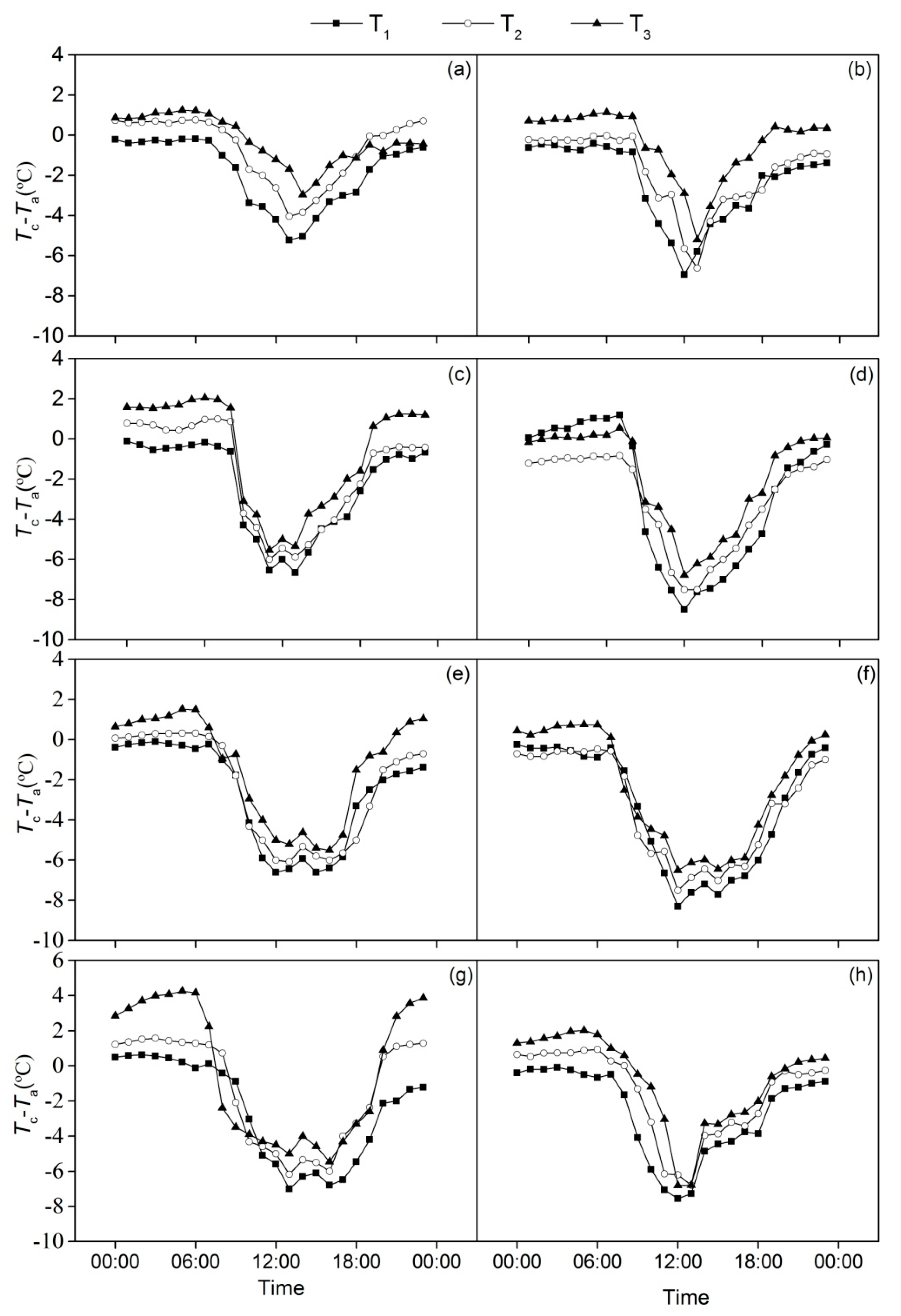
3.1.1. Daily Changes in the Leaf-Air Temperature Difference before and after Irrigation

The daily changes in Tc-Ta before and after irrigation under different stages were V-shaped curves (Figure 1). It could be observed that the Tc-Ta value of each treatment was basically negative the day before and after irrigation, which was consistent with the results of Sepaskhah [32]. At the flowering stage, the Tc-Ta value of each treatment began to decrease after 13:00 and remained stable at approximately 20:00 (Figure 1c). Tc-Ta reached a peak under the three treatments during the mature stage, which was −5.45~−7.01 °C (Figure 1g). Tc-Ta decreased rapidly between 16:00–19:00. On the one hand, the leaf temperature was affected by Ra and ground radiation; on the other hand, the specific heat capacity of water vapor is large, which made the leaf temperature decrease slowly. Thus, Tc-Ta appeared to decrease.
The peak of Tc-Ta after irrigation is higher than that before irrigation (Figure 1). Yeşim [33] found that the range of Tc-Ta during the entire growth period was −4 °C~3 °C, which was slightly smaller than the current experimental findings because Tc-Ta is affected by the crop variety, canopy resistance, leaf size, and canopy density [34]. Tc-Ta showed a “double-peak” curve under the three treatments during the fruit expansion stage. The first peak was slightly higher than the second because the leaf stomata were actively closed due to the high temperature (Figure 1f). When the environmental conditions cooled, the leaf stomata could not quickly recover to their original state. There was a certain lag, and the leaf temperature was still high, resulting in the peak of Tc-Ta being lower than the first peak. The peak of Tc-Ta at the mature stage developed at approximately 13:00 (Figure 1g,h). We concluded that the Tc-Ta of each treatment decreased as the water deficit increased because the leaf stomata tended to close under water stress, and the decrease in transpiration intensity would lead to a small amount of heat loss on the leaf surface; therefore, the leaf temperature was high, and Tc-Ta decreased [35]. Similar results were obtained by Rǔzica Stričević [36], who found that Tc-Ta between poplar and sorghum leaves increased as the water deficit increased.

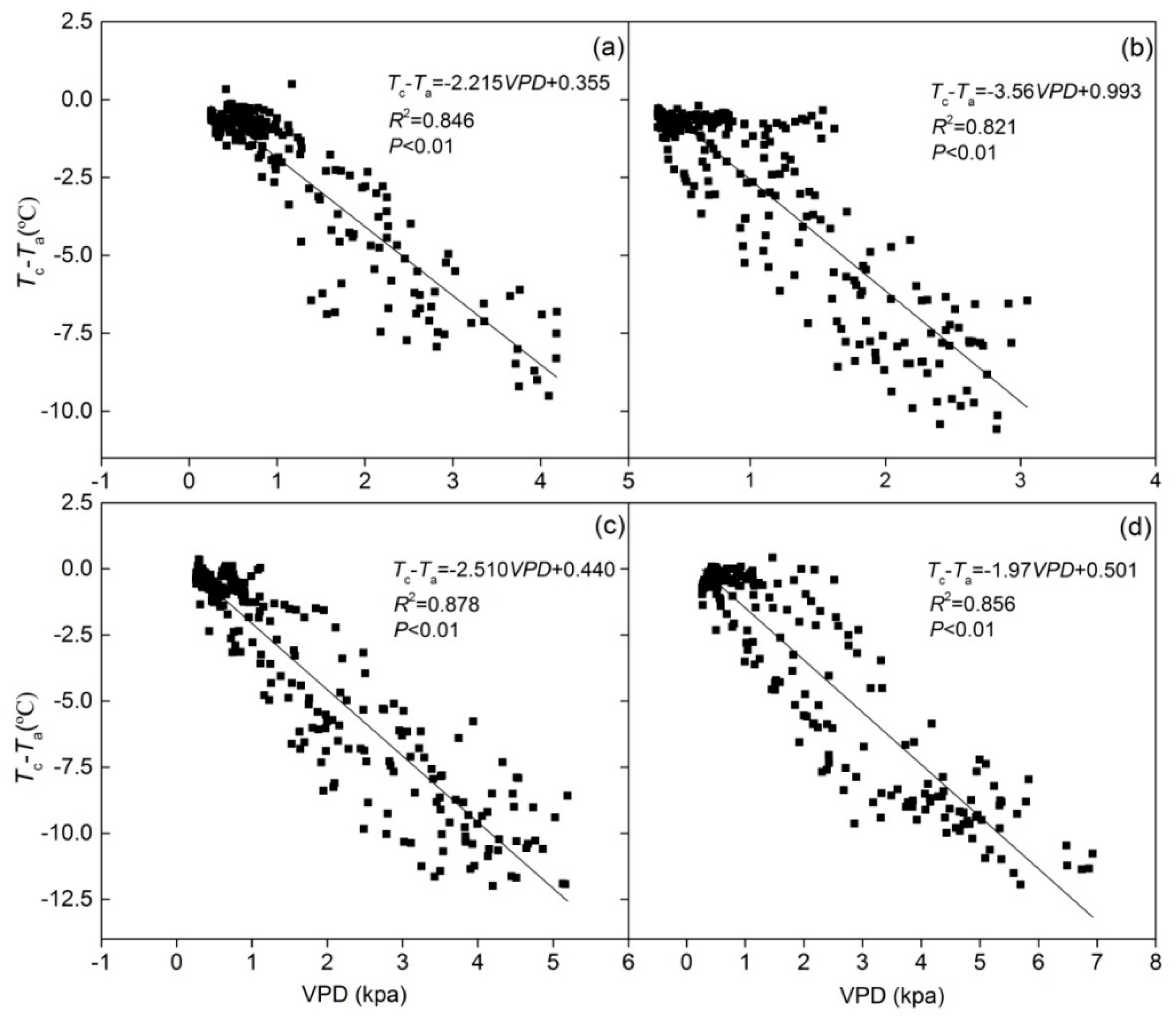
3.1.2. Relationship between Tc-Ta and Meteorological Factors

The correlation analysis of Tc-Ta with meteorological factors (Ta, Ra, RH and VPD) and leaf temperature are shown in Table 4. The positive correlation between Tc-Ta and Ra, Ta and VPD was significant (P < 0.05), and the negative correlation with RH was significant (P < 0.05) (Table 4). The results showed that meteorological factors had a significant effect on Tc-Ta. King and Shellie [37] obtained similar research conclusions. Moreover, Jensen et al. [38] believed that the main meteorological factor affecting Tc was Ra. This study indicated that Ra had the least correlation with Tc-Ta, which was mainly because the plastic roofs of greenhouses would block part of the Ra. Furthermore, Ra at night was zero; thus, the change in Tc was no longer affected by Ra. The correlation coefficients of Tc-Ta and Ra, Tc-Ta and RH decreased with the development of growth period, from 0.651–0.734 and 0.711–0.861 to 0.453–0.607 and 0.525–0.621, respectively (Table 4).

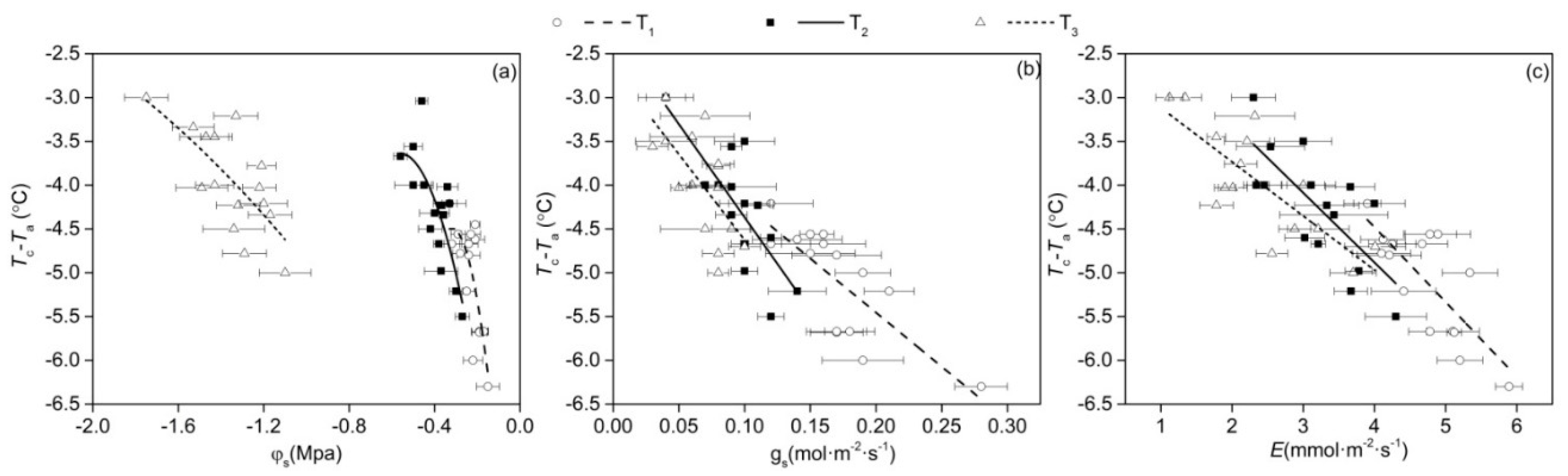
3.1.3. Relationship between Tc-Ta and Plant Water Status Indicators

The fitting diagrams of Tc-Ta with plant water status indictors ( φ s , gs, and E) under the three treatments are shown in Figure 2, and the coefficient of the fitting equation between Tc-Ta and plant water status index ( φ s , gs, and E) is shown in Table 5. The relationship between Tc-Ta and the plant water status indicators showed a correlation when dates were pooled together, and the correlation was significant among all treatments (P < 0.05), which indicates that Tc-Ta can reflect the water status of grapevines to a certain extent. The φ s , gs, and E values decreased with the decrease of Tc-Ta. It was easy to find that the relationship between φ s and Tc-Ta was a quadratic function curve (Figure 2a). Gonzalez-Dugo et al. [39] also believed that the relationship between the stem water potential and the CWSI was a quadratic function curve, consistent with the results of this paper. The gs and E values were linearly correlated with Tc-Ta (Figure 2b,c). Khorsandi et al. [35] reported that there is a significant and linear relationship between Tc-Ta and gs. In general, the relationships between Tc-Ta and gs and between Tc-Ta and E were higher, with R2 values ranging from 0.530–0.604 and from 0.545–0.623, respectively (Table 5).

3.2. Diagnosis of Grapevine Water Deficiency Based on the CWSI

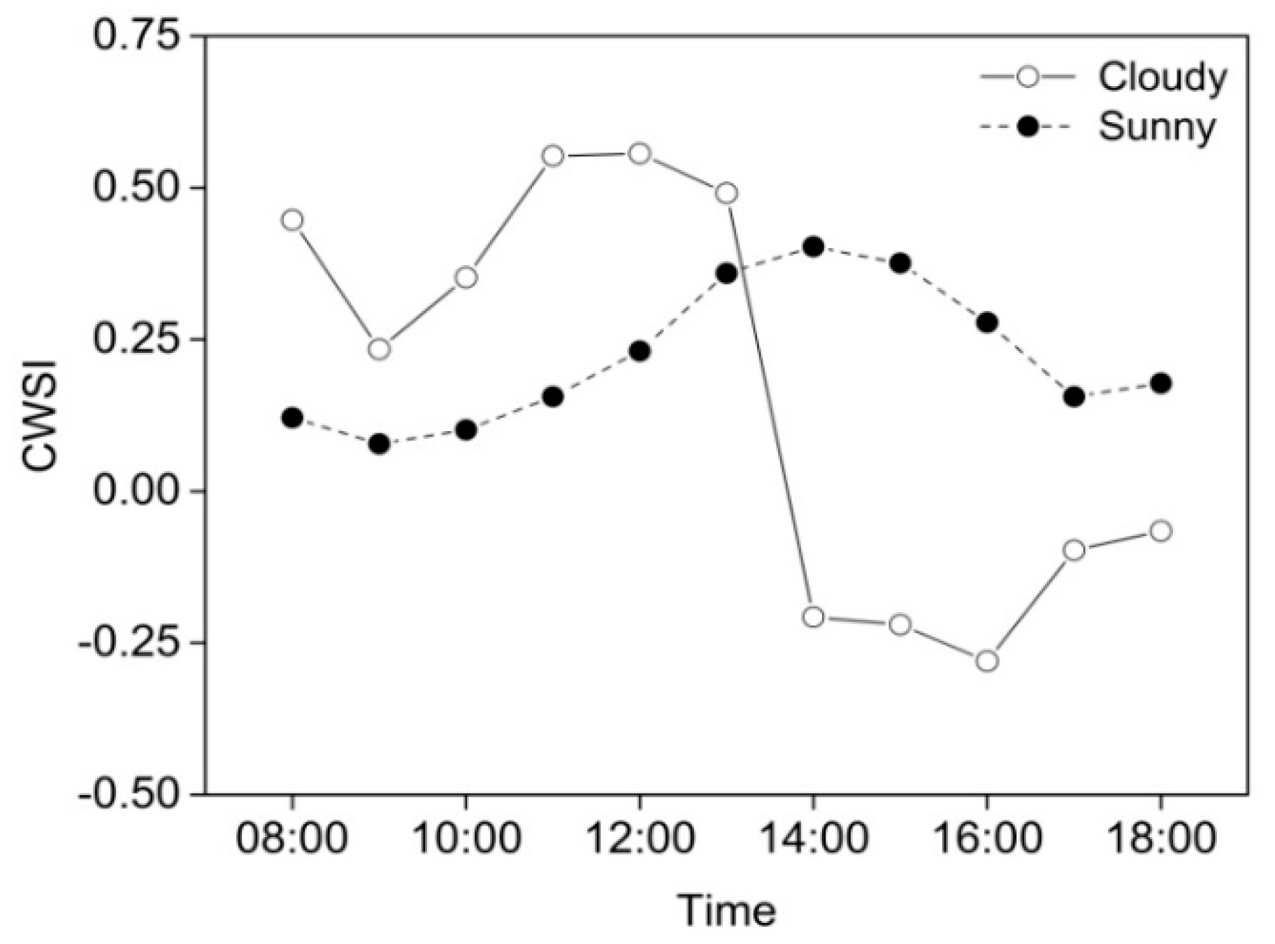
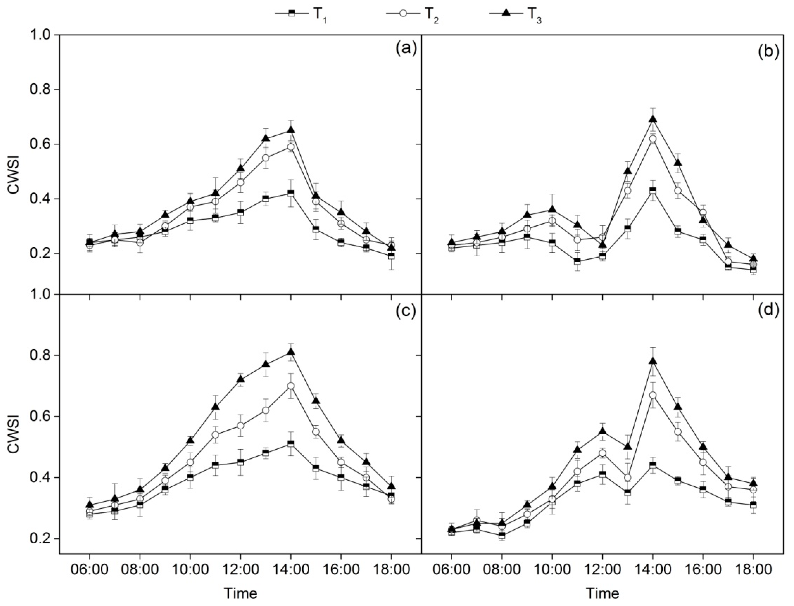
3.2.1. Daily Changes in the CWSI under Different Weather Conditions

The daily changes in the CWSI under the two weather conditions are shown in Figure 3. The fluctuation of the CWSI under T1 on sunny days was relatively stable (0.078–0.403) (Figure 3). Moreover, Jones [40] found that the leaf temperature of non-transpiration and full-transpiration could be used as the upper and lower limits of the canopy temperature, respectively. The change rule of the CWSI on cloudy days was similar to that on sunny days, but cloudy days showed a significantly larger range in magnitude than sunny days (−0.280–0.556). Gardner et al. [41] concluded that the stable CWSI values could be used to diagnose plant water deficiency, which is consistent with the results of this study. We concluded that the CWSI was more suitable for sunny weather, and the CWSI would be unstable on rainy days, which is also the reason why the CWSI model is limited as a suitable irrigation index [42,43].

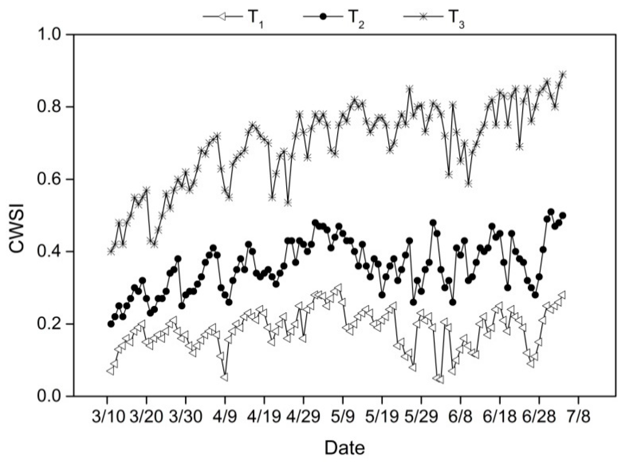
3.2.2. NWSB and CWSI

There was a significant negative correlation between Tc-Ta and VPD during different stages (Figure 4). Similar results were obtained by Khorsandi et al., who found that the negative correlation between Tc-Ta and VPD was significant [35]. The R2 value was the highest (0.878) during the fruit expansion stage (Figure 4c), which might be related to the changes in transpiration and photosynthesis during the reproductive stage of grapevines. Furthermore, the absolute value of the slope of the equation during the flowering stage was larger than that during the other stages (Figure 4b), which indicates that the transpiration ability of grapevines changes due to different growth conditions under different stages, thus resulting in different ranges of Tc decreases under the same VPD. Bellvert [44] established the upper (ul) and lower limit baselines (ll) of Pinot-noir grapevines as follows: ll = −1.709VPD + 2.534 and ul = 0.465 VPD + 6.125 (R2 = 0.83). Bellvert [45] also developed the ll equation of grapevines as follows: ll = −1.326 VPD + 3.111 (R2 = 0.424). However, differences in the crop varieties, management methods, soil moisture, and climate conditions will affect the upper and lower limit equations.
The daily changes in the CWSI under the three treatments during the different stages were inverted “V” curves that increased first and then decreased (Figure 5). The CWSI of the three treatments reached the maximum at approximately 14:00 during the different stages, and the peaks of the CWSI under the three treatments were the largest during the fruit expansion stage, ranging from 0.51 to 0.81 (Figure 5c). The CWSI under T1 was significantly lower than that under T2 and T3, indicating that the CWSI increased as the irrigation amount decreased (Figure 5). The results of this study confirmed the views of Sezen et al. [46] and of Colak and Yazar [47]. There were two peaks of the CWSI during the flowering and mature stages (Figure 5b,d), and the second peak was larger than the first peak. However, some studies [26,48] reported that the CWSI might exceed the range of 0~1.0. This might be caused by inconsistent baseline calculation methods. We concluded that the order of the CWSI for the three treatments during the entire growth period was T3 > T2 > T1, and 14:00 was the best observation time for the CWSI to reflect the water status of grapevines.
The CWSI value of the T3 treatment showed a zigzag upward trend, while the CWSI of the T1 and T2 treatments increased first and then decreased during the growing season (Figure 6 and Table 6). The CWSI values of the T1, T2, and T3 treatments were 0.07–0.30, 0.20–0.51, and 0.40–0.89 during the growing season (Figure 6). Bellvert [44] reported that the CWSI was occasionally negative under full irrigation treatment, which was not found in the results of this study. As can be seen in Figure 6, the CWSI was different in adjacent time periods, indicating that many external factors, including meteorological factors such as the wind speed, wind direction, clouds, VPD, Ta, and Ra, affect it [49]. The CWSI values of each treatment decreased after irrigation, and there were different degrees of lag (Figure 6). The reason is that stomatal conductance does not reach the maximum rapidly as the soil moisture changes after rewatering; rather, it recovers slowly under the influence of early water stress, so the leaf temperature is still high [50]. The seasonal mean CWSI values of the three treatments were 0.181, 0.350, and 0.677, respectively (Table 6). Bellvert and Girona [51] reported that the CWSI values under a full irrigation treatment were lower than 0.5, while those under a severe water deficit treatment were close to 1.0; the findings of this study agree with their results. Yazar et al. [52] evaluated the CWSI values of ergot seedless and flame seedless and suggested that crops should be irrigated when the CWSI values reached 0.30–0.35 in the Mediterranean area.

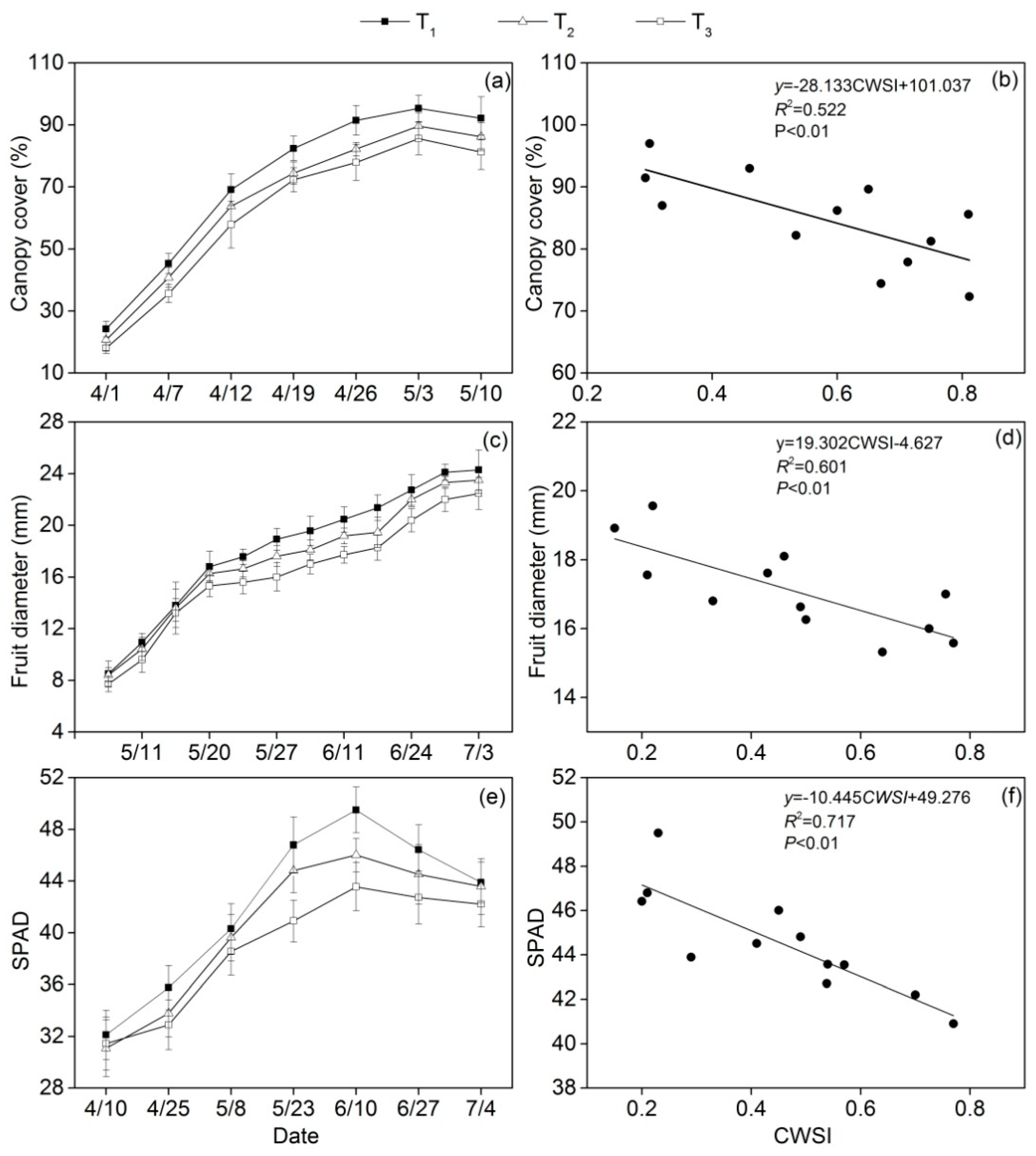
3.2.3. Relations between the CWSI and Canopy Cover, Fruit Diameter and SPAD

Many studies showed that the CWSI values are closely related to the leaf area index [53], photosynthetic index [54], which can be used as an indirect index to identify the drought tolerance of crops. Based on the above analysis, the correlations of the CWSI values with the canopy cover (CC), fruit diameter (FD), and SPAD of grapevines is shown in Figure 7. On May 3, the peaks of CC under the three treatments were 95.32% for T1, 89.65% for T2 and 85.61% for T3 (Figure 7a). The FD of the grapevines maintained a rapid growth trend before May 20, and there was no significant difference among the treatments (Figure 7c). After May 20, the FD under the three treatments increased with increasing irrigation amount and reached 22.45–24.28 mm at the end of the mature stage. In addition, regarding SPAD, different irrigation amounts had a more significant influence on SPAD from 8 May to 27 June. The maximum SPAD values under T1, T2, and T3 were 43.55, 46.01 and 49.50, respectively (Figure 7e).
As Figure 7b shows, the correlation of the CWSI with CC reached a very significant level (P < 0.01). The current experimental finding agreed with the results of other crops [55,56]. There was a very significant negative correlation between the CWSI and FD (Figure 7d). However, Orta et al. [57] reported that crop morphological size was limited owing to water deficit, and the decrease in crop assimilation was the main reason for the decrease in fruit quantity and diameter at the fruit development stage. There was a very significant negative correlation of the CWSI with SPAD (Figure 7f), and the determination coefficient reached 0.717. By analyzing the relationship of the CWSI and the growth and physiological indexes, we concluded that the CWSI could effectively reflect the water status of grapevines.

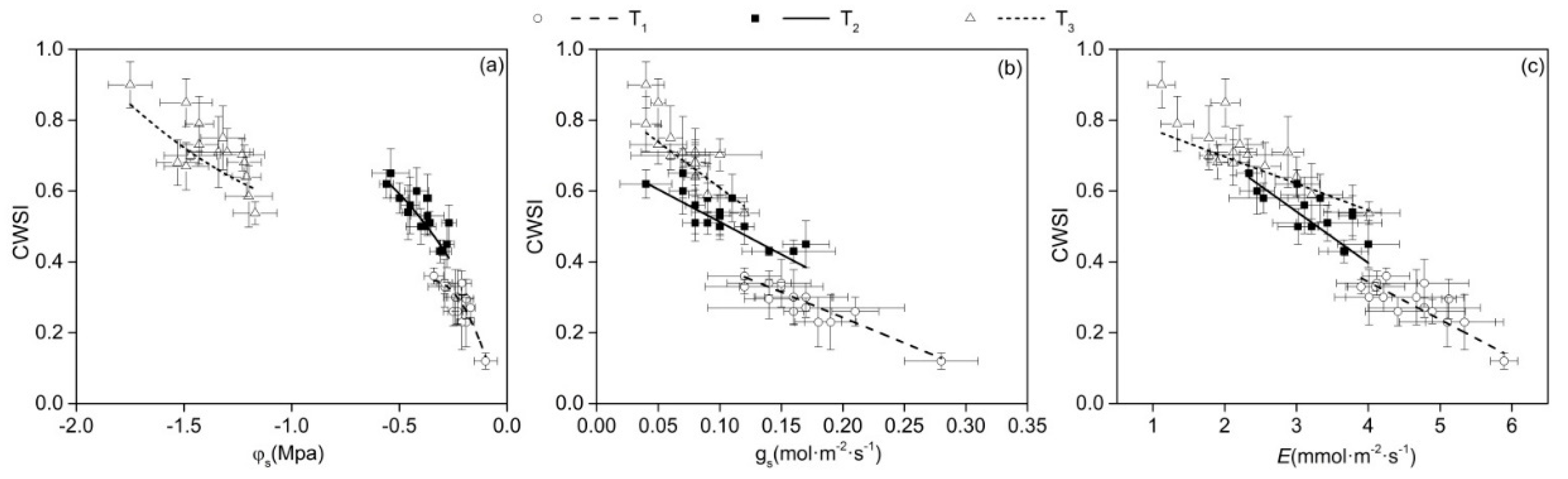
3.2.4. Relationship between the CWSI and the Plant Water Status Indicators

Soil moisture is the direct source of plant water. Drought stress will lead to decreases in the soil moisture absorption capacity of the root system and then cause the plant water status to decrease, which is an indirect and adaptive feature of plants to cope with the decrease of soil moisture [58]. To explore the relationship between the CWSI and soil moisture, the correlation between the CWSI and soil moisture at 0–40 cm and 40–80 cm was analyzed. The results showed that the fitting effect of the CWSI and soil moisture (0–40 cm) was sound, and the correlation was significant (P < 0.05) (Figure 8a). However, the R2 of the CWSI with soil moisture for the deep soil (40–80 cm) was relatively low (Figure 8b) and between 0.123 and 0.403. This indicates that the CWSI more suitably reflects the water status of shallow soil, which is beneficial to understanding the effect of drought stress on the plant water status to a certain extent.
The relationship between plant water status indictors ( φ s , gs and E) and CWSI were close (Figure 9), and the R2 were high (Table 7). Moreover, the relationships between CWSI and φ s , gs and E were significant at the level of P < 0.01, which indicated that CWSI is a suitable indicator for the diagnosis of plant water status. The relationship between gs and CWSI was the closest, the R2 was between 0.708 and 0.847, whereas the relationship between φ s E and CWSI was 0.565–0.730 and 0.569–0.711, respectively (Table 7). When the CWSI is compared to Tc-Ta as a proxy of the water status (by comparing the R2 and P values of the relationship of both indices to φ s , gs, and E, Table 5 and Table 7), it can be observed that the CWSI more accurately represents the crop water status. Compared to Tc-Ta, the performance of the CWSI is improved by considering the evaporative demand and the species-specific response of the relationship to VPD. These results are similar to the theoretical foundation of CWSI, demonstrating that the change of leaf temperature is mainly determined by the change of gs under water stress [59]. Under water stress, the stem and leaf water potential reached the lowest through stomatal regulation, which also explained that the correlation between CWSI and leaf, stem water potential and transpiration rate was not high. Berni et al. [60] reported that for olive trees, there is a linear relationship between CWSI and gs, the same results were also confirmed in nectarines [61]. The relationship between E and CWSI was weaker than that with gs (Table 7), although the transpiration rate of leaves depended largely on gs, the reason may be that transpiration rate is not only affected by stomatal conductance but also on the conductivity of the boundary layer [62].
In many previous studies to evaluate the applicability of CWSI, ψ s [39,63] or ψ l [61] is usually the most suitable indicator to determine the applicability of CWSI as an indicator of water status. However, many studies showed that the relationships between CWSI and plant water status indictors were not always linear, which is consistent with the results of this study (Figure 9a,b). For instance, linear and curvilinear relationships were reported for both grapevine [44,45] and peach [63].

4. Conclusions

It can be concluded that according to different NWSBs, the diurnal change in the CWSI among the three treatments was obviously different, and the best observation time of the CWSI value was 14:00 BJS. The CWSI value can be used to predict the canopy coverage, fruit diameter, and SPAD. Moreover, there was a reliable relationship between Tc-Ta and the plant water status indicators; however, the CWSI could more accurately monitor the water stress and assess the water status variability in grapevines in greenhouses. Stomatal conductance had the closest relationship with the CWSI, outperforming other widely used plant water status indicators such as the leaf water potential, stem water potential, and leaf transpiration rate.
Plant water status can be diagnosed by monitoring leaf temperature data. Meanwhile, CWSI is closely related to soil moisture content, it can be combined with plant water status and soil moisture content to guide crop irrigation based on CWSI. The response of plants to CWSI is affected by many factors under water stress, to carry out a successful irrigation schedule based on CWSI, the future research should also consider the influence of cultivation methods, climate conditions and other factors on CWSI, and the threshold of CWSI is further obtained when plants need irrigation under water stress. At present, CWSI is widely used in satellite remote sensing technology. The study of CWSI measured in the field can provide reference for CWSI based on satellite thermal infrared, the combination of CWSI by the two methods can diagnose plant water deficiency more accurately and predict irrigation schedule in future.

Author Contributions

C.R., X.H., W.W. and H.R. designed the experiments, C.R., T.S., Y.G. performed research and date analysis, C.R. wrote the manuscript with contributions from all authors. All authors have read and agreed to the published version of the manuscript.

Funding

This work was supported by the National Key Research and Development Program of China (2017YFD0201508), the National Natural Science Foundation of China (51179163), Shaanxi Key Science and Technology Innovation Team Project (2016KTZDNY-01–05).

Acknowledgments

The authors would like to acknowledge all the team members of key Laboratory of Agricultural Soil and Water Engineering in Arid and Semiarid Areas, Ministry of Education.

Conflicts of Interest

The authors declare that they have no conflict of interest.

References

  1. Zha, Q.; Xi, X.; He, Y.; Jiang, A. Transcriptomic analysis of the leaves of two grapevine cultivars under high-temperature stress. Sci. Hortic. 2020, 265, 109265. [Google Scholar] [CrossRef]
  2. Pellegrino, A.; Lebon, E.; Simonneau, T.; Wery, J. Towards a simple indicator of water stress in grapevine (Vitis vinifera L.) based on the differential sensitivities of vegetative growth components. Aust. J. Grape Wine Res. 2005, 11, 306–315. [Google Scholar] [CrossRef]
  3. Ezzhaouani, A.; Valancogne, C.; Pieri, P.; Amalak, T.; Gaudillère, J.P. Water economy by Italia grapevines under different irrigation treatments in a Mediterranean climate. J. Int. Sci. Vigne Vin 2007, 41, 131–140. [Google Scholar]
  4. Alves, I.; Pereira, L.S. Non-water-stressed baselines for irrigation scheduling with infrared thermometers: A new approach. Irrig. Sci. 2000, 19, 101–106. [Google Scholar] [CrossRef]
  5. Cohen, Y.; Alchanatis, V.; Meron, M.; Saranga, Y.; Tsipris, J. Estimation of leaf water potential by thermal imagery and spatial analysis. J. Exp. Bot. 2005, 56, 1843–1852. [Google Scholar] [CrossRef] [Green Version]
  6. Cohen, Y.; Alchanatis, V.; Prigojin, A.; Levi, A.; Soroker, V.; Cohen, Y. Use of aerial thermal imaging to estimate water status of palm trees. Precis. Agric. 2012, 13, 123–140. [Google Scholar] [CrossRef]
  7. Egea, G.; Padilla-Díaz, C.M.; Martinez-Guanter, J.; Fernández, J.E.; Perez-Ruiz, M. Assessing a crop water stress index derived from aerial thermal imaging and infrared thermometry in super-high density olive orchards. Agric. Water Manag. 2017, 187, 210–221. [Google Scholar] [CrossRef] [Green Version]
  8. Ballester, C.; Jiménez-Bello, M.; Castel, J.; Intrigliolo, D. Usefulness of thermo graphy for plant water stress detection in citrus and persimmon trees. Agric. For. Meteorol. 2013, 168, 120–129. [Google Scholar] [CrossRef]
  9. Roh, M.; Nam, Y.; Cho, M.; Yu, I.; Choi, G.; Kim, T. Environmental control in greenhouse based on phytomonitoring-leaf temperature as a factor controlling greenhouse environments. Acta Hortic. 2007, 761, 71–76. [Google Scholar] [CrossRef]
  10. Langton, F.; Horridge, J.; Hamer, P. Effects of the glasshouse environment on leaf temperature of pot chrysanthemum and dieffenbachia. Acta Hortic. 2000, 534, 75–84. [Google Scholar] [CrossRef]
  11. Idso, S.B.; Jackson, R.D.; Pinter, R.D.; Reginato, R.J.; Hatfield, J.L. Normalizing the stres-degree-day parameter for environmental variability. Agric. Meteorol. 1981, 24, 45–55. [Google Scholar] [CrossRef]
  12. Jackson, R.D.; Idso, S.B.; Reginato, R.J.; Pinter, P.J. Canopy temperature as a crop water stress indicator. Water Resour. Res. 1981, 17, 1133–1138. [Google Scholar] [CrossRef]
  13. Kanemasu, E.; Steiner, J.; Biere, A.; Worman, F.; Stone, J. Irrigation in the Great Plains. Agric. Water Manag. 1983, 7, 157–178. [Google Scholar] [CrossRef]
  14. William, S.B.; Mack, H.J. The possible use of the crop water stress index as an indicator of evapotranspiration deficits and yield reduıctions in sweet corn. J. Am. Soc. Hortic. Sci. 1989, 114, 542–546. [Google Scholar]
  15. Wanjura, D.F.; Upchurch, D.R.; Mahan, J.R. Automated irrigation based on threshold canopy tempearture. Am. Soc. Agric. Eng. 1992, 35, 145–152. [Google Scholar]
  16. Yazar, A.; Howell, T.A.; Dusek, D.A.; Copeland, K.S. Evaluation of crop water stress index for LEPA irrigated corn. Irrig. Sci. 1999, 18, 171–180. [Google Scholar] [CrossRef]
  17. O’Shaughnessy, S.A.; Evett, S.R.; Colaizzi, P.D.; Howell, T.A. A crop water stress index and time threshold for automatic irrigation scheduling of grain sorghum. Agric. Water Manag. 2012, 107, 122–132. [Google Scholar] [CrossRef] [Green Version]
  18. Köksal, E.S.; Üstün, H.; İlbeyi, A. Threshold values of leaf water potential and crop water stress index as an indicator of irrigation time for dwarf green beans. J. Agric. 2010, 24, 25–36. [Google Scholar]
  19. Köksal, E.S. Determination of the Effects of different irrigation level on sugarbeet yield, quality and physiology using infrared thermometer and spectroradiometer. Int. J. Mater Form. 2014, 7, 317–335. [Google Scholar]
  20. Argyrokastritis, I.G.; Papastylianou, P.; Alexandris, S. Leaf Water Potential and Crop Water Stress Index Variation for Full and Deficit Irrigated Cotton in Mediterranean Conditions. Agric. Agric. Sci. Procedia 2015, 4, 463–470. [Google Scholar] [CrossRef] [Green Version]
  21. Veysi, S.; Naseri, A.A.; Hamzeh, S.; Bartholomeus, H. A satellite based crop water stress index for irrigation scheduling in sugarcane fields. Agric. Water Manag. 2017, 189, 70–86. [Google Scholar] [CrossRef]
  22. Han, M.; Zhang, H.; Dejonge, K.C.; Comas, L.H.; Gleason, S.M. Comparison of three crop water stress index models with sap flow measurements in maize. Agric. Water Manag. 2018, 203, 366–375. [Google Scholar] [CrossRef]
  23. Jackson, R.D.; Reginato, R.J.; Idso, S.B. Wheat canopy temperature: A practical tool for evaluating water requirements. Water Resour. Res. 1977, 13, 651–656. [Google Scholar] [CrossRef]
  24. Nielsen, D.C. Scheduling irrigations for soybeans with the Crop Water Stress Index (CWSI). Field Crop. Res. 1990, 23, 103–116. [Google Scholar] [CrossRef]
  25. Emekli, Y.; Bastug, R.; Buyuktas, D.; Emekli, N.Y. Evaluation of a crop water stress index for irrigation scheduling of bermudagrass. Agric. Water Manag. 2007, 90, 205–212. [Google Scholar] [CrossRef]
  26. Stegman, E.C.; Soderlund, M. Irrigation Scheduling of Spring Wheat Using Infrared Thermometry. Trans. Chin. Soc. Agric. Eng. 1992, 35, 143–152. [Google Scholar] [CrossRef]
  27. Alderfasi, A.A.; Nielsen, D.C. Use of crop water stress index for monitoring water status and scheduling irrigation in wheat. Agric. Water Manag. 2001, 47, 69–75. [Google Scholar] [CrossRef]
  28. Erdem, Y.; Arin, L.; Erdem, T.; Polat, S.; Deveci, M.; Okursoy, H.; Gültaş, H.T. Crop water stress index for assessing irrigation scheduling of drip irrigated broccoli (Brassica oleracea L. var. italica). Agric. Water Manag. 2010, 98, 148–156. [Google Scholar] [CrossRef]
  29. Jackson, S.H. Relationships between normalized leaf water potential and crop water stress index values for acala cotton. Agric. Water Manag. 1991, 20, 109–118. [Google Scholar] [CrossRef]
  30. Allen, R. Using the FAO-56 dual crop coefficient method over an irrigated region as part of an evapotranspiration intercomparison study. J. Hydrol. 2000, 229, 27–41. [Google Scholar] [CrossRef]
  31. Jackson, R.D.; Kustas, W.P.; Choudhury, B.J. A reexamination of the crop water stress index. Irrig. Sci. 1988, 9, 309–317. [Google Scholar] [CrossRef]
  32. Sepaskhah, A.; Kashefipour, S. Relationships between leaf water potential, CWSI, yield and fruit quality of sweet lime under drip irrigation. Agric. Water Manag. 1994, 25, 13–21. [Google Scholar] [CrossRef]
  33. Ahi, Y.; Orta, H.; Gündüz, A.; Gültaş, H.T. The Canopy Temperature Response to Vapor Pressure Deficit of Grapevine cv. Semillon and Razaki. Agric. Agric. Sci. Procedia 2015, 4, 399–407. [Google Scholar] [CrossRef] [Green Version]
  34. Leuzinger, S.; Körner, C. Tree species diversity affects canopy leaf temperatures in a mature temperate forest. Agric. For. Meteorol. 2007, 146, 29–37. [Google Scholar] [CrossRef]
  35. Khorsandi, A.; Hemmat, A.; Mireei, S.A.; Amirfattahi, R.; Ehsanzadeh, P. Plant temperature-based indices using infrared thermography for detecting water status in sesame under greenhouse conditions. Agric. Water Manag. 2018, 204, 222–233. [Google Scholar] [CrossRef]
  36. Stričević, R.; Čaki, E. Relationships between available soil water and indicators of plant water status of sweet sorghum to be applied in irrigation scheduling. Irrig. Sci. 1997, 18, 17–21. [Google Scholar] [CrossRef]
  37. King, B.; Shellie, K. Wine grape cultivar influence on the performance of models that predict the lower threshold canopy temperature of a water stress index. Comput. Electron. Agric. 2018, 145, 122–129. [Google Scholar] [CrossRef]
  38. Jensen, H.E.; Svendsen, H.; Jensen, S.E.; Mogensen, V.O. Canopy-air temperature of crops grown under different irrigation refimes in a temperate humid climate. Irrig. Sci. 1990, 11, 181–188. [Google Scholar] [CrossRef]
  39. González-Dugo, V.; Zarco-Tejada, P.J.; Fereres, E. Applicability and limitations of using the crop water stress index as an indicator of water deficits in citrus orchards. Agric. For. Meteorol. 2014, 94–104. [Google Scholar] [CrossRef]
  40. Jones, H.G. Use of infrared thermometry for estimation of stomatal conductance as a possible aid to irrigation scheduling. Agric. For. Meteorol. 1999, 95, 139–149. [Google Scholar] [CrossRef]
  41. Gardner, B.R.; Nielsen, D.C.; Shock, C.C. Infrared thermometry and the crop water stress index. II. Sampling procedures and interpretation. J. Prod. Agric. 1992, 5, 466–475. [Google Scholar] [CrossRef]
  42. Jones, H.G. Irrigation scheduling: Advantages and pitfalls of plant-based methods. J. Exp. Bot. 2004, 55, 2427–2436. [Google Scholar] [CrossRef] [PubMed] [Green Version]
  43. Al-Faraj, A.; Meyer, G.E.; Horst, G.L. A crop water stress index for tall fescue (Festuca arundinacea Schreb.) irrigation decision-making—A traditional method. Comput. Electron. Agric. 2001, 31, 107–124. [Google Scholar] [CrossRef]
  44. Bellvert, J.; Marsal, J.; Girona, J.; Zarco-Tejada, P.J. Seasonal evolution of crop water stress index in grapevine varieties determined with high-resolution remote sensing thermal imagery. Irrig. Sci. 2015, 33, 81–93. [Google Scholar] [CrossRef]
  45. Bellvert, J.; Zarco-Tejada, P.J.; Girona, J.; Fereres, E. Mapping crop water stress index in a ‘Pinot-noir’ vineyard: Comparing ground measurements with thermal remote sensing imagery from an unmanned aerial vehicle. Precis. Agric. 2014, 15, 361–376. [Google Scholar] [CrossRef]
  46. Sezen, S.M.; Yazar, A.; Daşgan, Y.; Yucel, S.; Akyıldız, A.; Tekin, S.; Akhoundnejad, Y. Evaluation of crop water stress index (CWSI) for red pepper with drip and furrow irrigation under varying irrigation regimes. Agric. Water Manag. 2014, 143, 59–70. [Google Scholar] [CrossRef]
  47. Çolak, Y.B.; Yazar, A. Evaluation of crop water stress index on Royal table grape variety under partial root drying and conventional deficit irrigation regimes in the Mediterranean Region. Sci. Hortic. 2017, 224, 384–394. [Google Scholar] [CrossRef]
  48. Yuan, G.; Luo, Y.; Sun, X.; Tang, D. Evaluation of a crop water stress index for detecting water stress in winter wheat in the North China Plain. Agric. Water Manag. 2004, 64, 29–40. [Google Scholar] [CrossRef]
  49. Chen, J.; Lin, L.; Lu, G. An index of soil drought intensity and degree: An application on corn and a comparison with CWSI. Agric. Water Manag. 2010, 97, 865–871. [Google Scholar] [CrossRef]
  50. Sala, O.; Lauenroth, W.; Parton, W. Plant recovery following prolonged drought in a shortgrass steppe. Agric. Meteorol. 1982, 27, 49–58. [Google Scholar] [CrossRef]
  51. Bellvert, J.; Girona, J. The use of multispectral and thermal images as a tool for irrigation scheduling in vineyards. Options Mediterr. Ser. B. Stud. Res. 2012, 67, 131–137. [Google Scholar]
  52. Yazar, A.; Tangolar, S.; Sezen, S.M.; Colak, Y.B.; Gencel, B.; Ekbic, H.B.; Sabır, A. New Approaches in Vineyard Irrigation Management: Determining Optimal Irrigation Time Using Leaf Water Potential for High Quality Yield Under Mediterranean Conditions; Project No: TOVAG-1060747; Turk. Science and Research Council (TUBITAK): Ankara, Turkey, 2010; p. 100.
  53. Kirnak, H.; Irik, H.; Unlukara, A. Potential use of crop water stress index (CWSI) in irrigation scheduling of drip-irrigated seed pumpkin plants with different irrigation levels. Sci. Hortic. 2019, 256, 108608. [Google Scholar] [CrossRef]
  54. Pou, A.; Diago, M.P.; Medrano, H.; Baluja, J.; Tardaguila, J. Validation of thermal indices for water status identification in grapevine. Agric. Water Manag. 2014, 134, 60–72. [Google Scholar] [CrossRef]
  55. Turner, N.; Hearn, A.; Begg, J.; Constable, G. Cotton (Gossypium hirsutum L.) Physiological and morphological responses to water deficits and their relationship to yield. Field Crop. Res. 1986, 14, 153–170. [Google Scholar] [CrossRef]
  56. Aladenola, O.; Madramootoo, C. Effect of different water application on yield and water use of bell pepper under greenhouse conditions. In Proceedings of the NABEC-CSBE/SCGAB 2012 Joint Meeting and Technical Conference Northeast Agricultural & Biological Engineering Conference Canadian Society for Bioengineering, Orillia, ON, USA, 15–18 July 2012. [Google Scholar]
  57. Orta, A.; Erdem, Y.; Erdem, T. Crop water stress index for watermelon. Sci. Hortic. 2003, 98, 121–130. [Google Scholar] [CrossRef]
  58. Kramer, P.J. Changing concepts regarding plant water relations. Plant Cell Environ. 1988, 11, 565–568. [Google Scholar] [CrossRef]
  59. Maes, W.H.; Steppe, K. Estimating evapotranspiration and drought stress with ground-based thermal remote sensing in agriculture: A review. J. Exp. Bot. 2012, 63, 4671–4712. [Google Scholar] [CrossRef] [Green Version]
  60. Berni, J.; Zarco-Tejada, P.J.; Sepulcre-Cantó, G.; Fereres, E.; Villalobos, F. Mapping canopy conductance and CWSI in olive orchards using high resolution thermal remote sensing imagery. Remote Sens. Environ. 2009, 113, 2380–2388. [Google Scholar] [CrossRef]
  61. Bellvert, J.; Marsal, J.; Girona, J.; Gonzalez-Dugo, V.; Fereres, E.; Ustin, S.L.; Zarco-Tejada, P.J. Airborne Thermal Imagery to Detect the Seasonal Evolution of Crop Water Status in Peach, Nectarine and Saturn Peach Orchards. Remote Sens. 2016, 8, 39. [Google Scholar] [CrossRef] [Green Version]
  62. Jones, H.G. Plants and Microclimate: A Quantitative Approach to Environmental Plant Physiology; Cambridge University Press: Cambridge, UK, 1993; Volume 142, pp. 381–382. [Google Scholar]
  63. Gonzalez-Dugo, V.; Zarco-Tejada, P.J.; Nicolás, E.N.; Nortes, P.A.; Alarcón, J.J.; Intrigliolo, D.S.; Fereres, E. Using high resolution UAV thermal imagery to assess the variability in the water status of five fruit tree species within a commercial orchard. Precis. Agric. 2013, 14, 660–678. [Google Scholar] [CrossRef]
Figure 1. Daily change in the leaf-air temperature difference before and after irrigation at different stages. (a,b) represent the vegetative stage; (c,d) represent the flowering stage; (e,f) represent the fruit expansion stage; and (g,h) represent the mature stage. (a,c,e), and (g) represent Tc-Ta before irrigation, while (b,d,f,h) represent Tc-Ta after irrigation. T1 represents 100% M, T2 represents 80% M, T3 represents 60%.
Horticulturae 06 00086 g001
Figure 2. Relationships between Tc-Ta and plant-based water status indicators for three treatments. (a) stem water potential ( φ s ), (b) stomatal conductance (gs) and (c) leaf transpiration rate (E) for T1, T2 and T3 treatment. The different lines represent the fitting regression lines to the date. T1 represents 100% M, T2 represents 80% M, T3 represents 60%.
Horticulturae 06 00086 g002
Figure 3. Daily change in the CWSI under different weather conditions.
Horticulturae 06 00086 g003
Figure 4. NWSB of the CWSI at different stages: (a) represents the vegetative stage, (b) represents the flowering stage, (c) represents the fruit expansion stage, and (d) represents the mature stage.
Horticulturae 06 00086 g004
Figure 5. Daily changes of the CWSI under the three treatments during different stages. (a) represents the vegetative stage, (b) represents the flowering stage, (c) represents the fruit expansion stage, and (d) represents the coloring mature stage. Date are means ± SE of three replicates. T1 represents 100% M, T2 represents 80% M, T3 represents 60%.
Horticulturae 06 00086 g005
Figure 6. Time evolution of the CWSI during the growing season. T1 represents 100% M, T2 represents 80% M, T3 represents 60%.
Horticulturae 06 00086 g006
Figure 7. The fitting chart of the CWSI with canopy cover, fruit diameter, and SPAD. (a,c,e) represent the change in the canopy cover, fruit diameter, and SPAD, respectively, and (b,d,f) represent the fitting equations of the above indexes and the CWSI, respectively. Data are the means ± SE of three replicates. T1 represents 100% M, T2 represents 80% M, T3 represents 60%.
Horticulturae 06 00086 g007
Figure 8. The relationship between the CWSI and the soil moisture of different layers under different treatments. (a) represents the relationship between soil moisture content of 0–40 cm and CWSI; (b) represents the relationship between soil moisture content of 0–80 cm and CWSI. T1 represents 100% M, T2 represents 80% M, T3 represents 60%.
Horticulturae 06 00086 g008
Figure 9. The relationship between CWSI and (a) stem water potential ( φ s ), (b) stomatal conductance (gs) and (c) leaf transpiration rate (E) for T1, T2 and T3 treatment. The different lines represent the fitting regression lines to the date. T1 represents 100% M, T2 represents 80% M, T3 represents 60%.
Horticulturae 06 00086 g009
Table 1. Meteorological data of different cultivation stages during the growing season.
Cultivation StageTaRaRHVPD
vegetative stage18.8301.053.80.33
flowering stage19.7327.950.40.35
fruit expansion stage22.3421.151.20.34
coloring mature stage25.1362.355.70.32
Note: Ta (°C): air temperature; Ra (w/m2): solar radiation; RH (%): relative humidity; VPD (kpa): vapor pressure deficit.
Table 2. Physical properties of the soil.
Depth (cm)Textural AnalysisFC (g·g−1)PWP (g·g−1)Bulk Density (g·cm−3)
Sand (%)Clay (%)Silt (%)Texture Class
0–4087.545.277.19Aeolian soil13.182.311.64
40–8070.2319.5310.24Sandy loam17.456.381.46
Note: FC: field capacity; PWP: permanently wilting point.
Table 3. Irrigation amount of grapevine under different cultivation stages.
Cultivation StageIrrigation DateIrrigation Amount (m3∙ha)
T1T2T3
vegetative stage3/11293.61234.80176.02
3/19293.61234.65175.55
3/27293.60234.60175.34
4/06293.62234.65175.62
Flowering stage4/15341.40273.05204.60
4/25341.39273.04204.15
Fruit expansion stage5/05341.39273.00204.20
5/13341.37272.58204.14
5/20341.42272.69204.47
5/27341.41273.10204.34
Coloring mature stage6/05293.60234.50175.59
6/15293.61234.55176.30
Total irrigation amount381030452280
Table 4. The correlation of leaf-air temperature difference with meteorological factors and leaf temperature.
Cultivation StageTreatmentTaRaRHVPDLeaf Temperature
Vegetative stageT10.843 **0.651 **−0.711 **0.947 **0.824 **
T20.802 **0.708 **−0.861 **0.954 **0.764 **
T30.783 **0.734 **−0.716 **0.956 **0.870 **
Flowering stageT10.826 **0.641 **−0.741 **0.831 **0.453 *
T20.879 **0.675 **−0.775 **0.839 **0.615 **
T30.605 **0.531 *−0.631 *0.644 **0.579 **
Fruit expansion stageT10.865 **0.607 **−0.661 *0.864 **0.675 **
T20.885 **0.570 **−0.584 **0.862 **0.702 **
T30.764 **0.537 **−0.563 **0.800 **0.636 **
Mature stageT10.838 **0.607 **−0.621 *0.813 **0.545 **
T20.760 **0.599 **−0.525 *0.665 **0.525 *
T30.627 **0.453 *−0.545 **0.709 **0.665 **
Note: * Correlation is significant at the 0.05 level. ** Correlation is significant at the 0.01 level. Ta (°C): air temperature; Ra (w/m2): solar radiation; RH (%): relative humidity; VPD (kpa): vapor pressure deficit.
Table 5. Regression coefficient and accuracy evaluation of fitting equation between Tc-Ta and plant water status index.
TreatmentIndicatorabcR2P
T1φs−58.497−37.298−10.4370.5870.005
gs −12.979−2.9140.6040.001
E −0.898−0.8210.5810.001
T2φs−19.704−22.245−9.9130.6110.003
gs −21.694−2.2250.6000.001
E −0.838−1.5470.5450.002
T3φs−0.670−4.340−8.5960.5110.014
gs −23.023−2.3890.5300.008
E −0.628−2.4500.623< 0.001
Note: “a” represents the coefficient of the quadratic term; “b” represents the coefficient of the first-order term; “c” represents the constant.
Table 6. Montly and seasonal mean CWSI values for the treatments.
MonthsMean CWSI
T1T2T3
March0.1590.2750.511
April0.1830.3580.668
May0.2170.3860.761
June0.1660.3800.766
Seasonal mean CWSI0.1810.3500.677
Table 7. Regression coefficient and accuracy evaluation of fitting equation between CWSI and plant water status index.
TreatmentIndicatorabcR2P
T1φs−2.801−2.110−0.0450.730<0.001
gs −1.4060.5190.847<0.001
E −0.0870.6880.663<0.001
T2φs0.069−0.5600.2980.7020.001
gs −1.6120.6960.708<0.001
E −0.0990.8530.5690.001
T3φs−0.095−0.699−0.0690.5650.007
gs −3.4810.9600.733<0.001
E −0.1030.9450.711<0.001
Note: “a” represents the coefficient of the quadratic term; “b” represents the coefficient of the first-order term; “c” represents the constant.
Publisher’s Note: MDPI stays neutral with regard to jurisdictional claims in published maps and institutional affiliations.

