

Study on Scale-Up of Anaerobic Fermentation Mixing with Different Solid Content
1
Wenzhou Key Laboratory of Novel Optoelectronic and Nanomaterials, Institute of Wenzhou, Zhejiang University, Wenzhou 325036, China
2
College of Energy Engineering, Zhejiang University, Hangzhou 310027, China
*
Author to whom correspondence should be addressed.
Fermentation 2023, 9(4), 375; https://doi.org/10.3390/fermentation9040375
Submission received: 24 March 2023
/
Revised: 11 April 2023
/
Accepted: 11 April 2023
/
Published: 14 April 2023
(This article belongs to the Topic Bioreactors: Control, Optimization and Applications - 2nd Volume)
Abstract
:The scale-up technology of anaerobic fermentation stirring equipment is worthy of attention. Computational fluid dynamics (CFD) simulations were used to study the scale-up of anaerobic fermentation mixing under different solid content conditions. The applicability of different scale-up criteria was analyzed by investigating the relative parameters, such as the blade tip speed and the Reynolds number. On this basis, the scale-up index was optimized and verified. The results revealed the applicability of five common scale-up criteria under different solid content conditions. When the solid content is less than 5%, the anaerobic fermentation tank should be scaled up according to the same Weber number. When the solid content is between 5% and 10%, the anaerobic fermentation tank should be scaled up according to the same blade tip speed; it was especially suitable for anaerobic fermentation and other conditions that limit the shear rate. Scaling up according to the Reynolds number was not recommended due to the poor mixing effect. When the scale-up index x reached 0.75, there was no need to further reduce it. For anaerobic fermentation systems, the suitable scale-up indices selected for 5%, 10%, and 15% solid content were 1.1, 1, and 0.75, respectively.
1. Introduction
Anaerobic fermentation is a process that converts organic matter (feces, straw, weeds, etc.) into combustible gases, such as methane, and other usable products (carbon dioxide, alcohol, acids, etc.) through the catabolism of various microorganisms under a specific temperature (28~38 °C) and humidity (40~60%) environment [1,2,3]. Treating organic waste to produce biogas through anaerobic fermentation process is a biomass energy technology to control environmental pollution, reduce carbon emissions, and provide renewable energy. In anaerobic fermentation, mechanical stirring is often used to accelerate the microbial growth and metabolic reactions [4,5]. Stirring can improve the efficiency of anaerobic fermentation of biogas and significantly increase the gas production rate and pollutant removal rate [6,7]. Under the global trend of energy savings and emissions reduction, the scale of anaerobic fermentation production has great development potential. Most available facilities worldwide are lab-scale (29%) or pilot-scale (41%), while there are far fewer demo-scale (15%) and commercial-scale (16%) facilities, which cannot meet the current demand [8]. Hence, the research on the scale-up technology of anaerobic fermentation stirring has become essential.
According to different production requirements, scale-up technology can be divided into five types: geometric similarity, dynamic similarity, kinematic similarity, thermal similarity, and chemical similarity, which respectively correspond to the size ratio, the structural force ratio, the flow rate ratio, the fluid temperature ratio, and the corresponding concentration ratio before and after scaling up. In general, the primary condition for scale-up of stirring equipment is geometric similarity. Industrial production is generally based on laboratory research results; then, industrial models are designed according to the geometric similarity method. However, due to the complexity of the fluid flow, it is usually challenging to achieve the same flow state on both a laboratory scale and an industrial scale [9]. Therefore, selecting key process features for the industrial scene is necessary, as is then choosing the corresponding scale-up criteria. The most commonly used scale-up criteria for solid-liquid mixing systems can be obtained through Equation (1) [10]. The scale-up indicators include unit volume power, blade tip speed, Reynolds number, rotational speed, Weber number, etc. It can be easily seen from Equation (1) that, when the reacting tank size is enlarged, the working speed required to achieve the same mixing effect tends to decrease. A slight change in the x value can significantly change the power consumption and dispersion effects of the solid-liquid mixing system.
where x is the scale-up index; and NS, NL, DS, and DL are the rotational speed and the diameter of the stirring tanks before and after scaling up, respectively.
The key to the geometric similarity method is selecting scale-up criteria suitable for different industrial scenes. Different scale-up criteria determine different x values in Equation (1). The corresponding scale-up indices of different criteria are shown in Table 1.
Many experimental and numerical studies have been conducted to investigate the scale-up of solid-liquid mixing systems. Montante et al. [11] used multi-impeller stirring tanks with similar geometric shapes to obtain the same solid concentration distribution. The appropriate scale-up index x under this condition was 0.93, closer to the scale-up criterion with the same blade tip speed (x = 1) rather than constant unit volume power (x = 2/3). Zhou et al. [12] found that the velocity field was similar before and after scaling up according to the same blade tip speed. The solid concentration distribution in most regions of the tank was relatively uniform, with a high local solid volume fraction only appearing at the bottom of the stirring tank and near the baffle. Harrison et al. [13] found that, under constant blade tip speed conditions, the unit volume power of the tank after scaling up would increase. When the unit volume power or the blade tip speed was constant, the small tank was more uniform than the larger one. However, with the increase in the solid volume fraction, the solid concentration distribution of the tank scaled up worsened. Jafari et al. [14] studied the effects of impeller type, blade off-bottom distance, and solid volume fraction on the solid concentration distribution characteristics in a dense solid-liquid system using the optical fiber probe method. Furthermore, the methods used to reproduce the lab-scale solid concentration distribution in industrial systems were evaluated, such as the same unit volume power method, the same blade tip speed method, the Montante method [11], and the Buurman method [15]. It was found that none of them was fully applicable. Therefore, exploring the most appropriate scale-up criteria for anaerobic fermentation mixing equipment under different solid volume fraction conditions is necessary to reproduce the solid concentration distribution of a lab-scale tank.
In this paper, a double-layer, two-pitched blade impeller, widely used in anaerobic fermentation, was selected. Through numerical simulation, the application of five common scale-up criteria was investigated. The appropriate scale-up index was optimized and determined for anaerobic fermentation systems with different solid content.
2. Materials and Methods
2.1. Experimental Setups
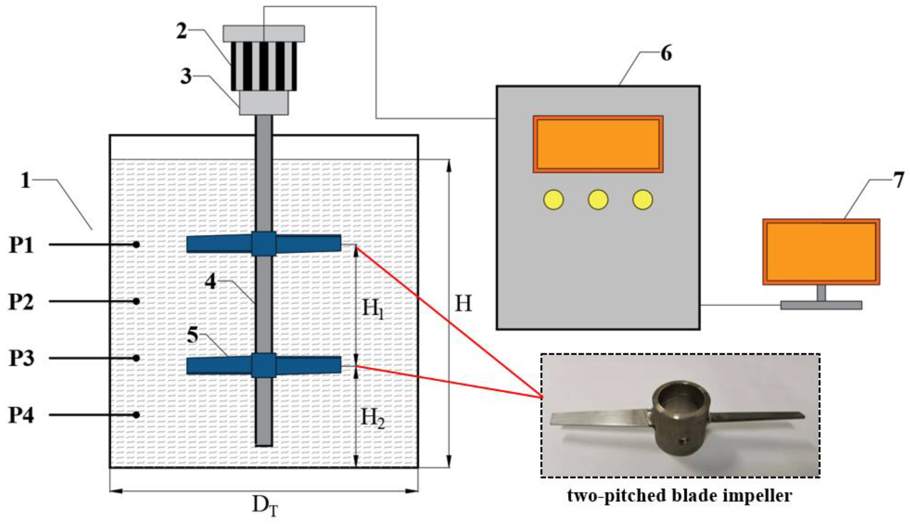
A particular experimental device was built to verify the accuracy of the numerical simulation, as shown in Figure 1. The stirring tank was a cylinder with a flat bottom, a diameter of 380 mm, and a total volume of 43.1 L. The liquid level height (H) during the experiment was always equal to the diameter of the tank (DT). The stirring tank was made of transparent organic glass, with holes for optical fiber probes on the tank body. To avoid the influence of external light on the measurement of the optical fiber probe, the whole stirring tank was wrapped with a black shading cloth during the experiment. A light shielding plate was also used to block the light above the stirring tank.
A double-layer impeller, composed of two-pitched blades, was selected as the research object in the experiment because the two-pitched blade impeller has lower power consumption and higher discharge at the same speed, compared with other impellers, such as the two-straight blades impeller, the Ruston impeller, and the propeller. In addition, the required speed of the double-layer impeller is significantly lower than that of the single-layer impeller with the same mixing effect, decreasing the shear rate [16]. Additionally, the double-layer impeller increases the mixing area and improves the mixing effect of the whole area in the stirring tank [17]. The structure of the two-pitched blade impeller is shown in Figure 1, with the diameter of a 152-mm blade. During the experiment, the distance between two impellers (H1) could be changed, and the lower impeller off-bottom distance (H2) was adjusted by controlling the lifting of the tank.
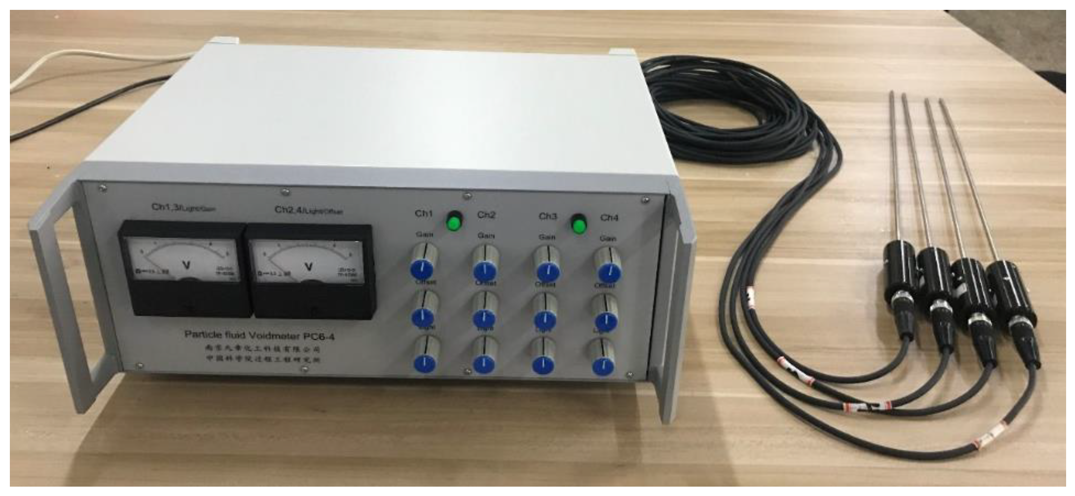
Based on the optical fiber probe method [18,19], the PC-6M particle concentration analyzer was used to measure the local solid volume fraction, as shown in Figure 2. The detection light was emitted to the tank through the light source, and it was reflected to the probe when encountering particles, at which point the probe transmitted the signal to the measuring instrument and converted it into a voltage value. The voltage value was transformed into the particle concentration value through the calibrated volt-particle concentration curve before the experiment [20]; finally the particle concentration value was displayed on the computer in real time. When using the optical fiber probe, it should be noted that the probe was horizontal and inserted at a depth of no more than 5 mm to avoid collision with the blade. Four measuring points were established during the experiment. The distance between the bottom probe and the bottom of the tank was 40 mm, and the distance between each measuring point was 100 mm.
Considering that the main purpose of this study was to maintain the mixing effect in the tank before and after enlarging the anaerobic fermentation mixing tank, and the reaction involved was a straw fermentation reaction, the experiment system could be simplified to a solid-liquid two-phase system. In the experiment, as a cheap and easily available material, malt syrup aqueous solution was selected as the liquid phase, composed of malt syrup at a concentration of 75% and water. The malt syrup aqueous solution in the experiment required a viscosity of 0.3 Pa·s and a density of 1337.5 kg/m3. Special consideration was given to the hydrophobicity, density and particle size of the material in the selection of the experimental solid phase used to characterize actual straw particles. As a hydrophobic material, polyformaldehyde particles were selected as the solid phase with a density of 1500 kg/m3, which was the same as the density of actual straw particles and was slightly heavier than the malt syrup aqueous solution prepared. Since the particle size significantly impacts mixing effects, particles similar to those in actual straw anaerobic fermentation scenes were selected, with an average particle size of 3.10 mm. As one of the critical factors in this study, the solid volume fraction (Co) had three conditions: 5%, 10%, and 15%. During the experiment, this factor could be prepared according to the requirement.
During the experiment, the rotating speed of the impeller was adjusted at intervals of 50 rpm. After the system was stable, the solid volume fraction at each monitoring point (Ci) was measured using the optical fiber probe. The real-time torque measured by the torque sensor was used to calculate the stirring power. To ensure the accuracy of the data, measurements were repeated at least three times in each group.
2.2. Simulation Methods
The model had two scales: lab test and pilot test. The size of the lab test was precisely the same as that of the experimental tank. Based on the lab test, the geometric similarity method was used to design the pilot test. The pilot test size was scaled up by 1.3 times that of the lab test, including mechanical components, such as the tank body, shaft, and blades. The specific parameters are shown in Table 2.
There are Euler–Euler and Euler–Lagrange methods for the study of multiphase flow. The Euler–Lagrange model regards the liquid phase as continuous fluid and the solid phase as discrete particles, between which there can be the exchange of mass, momentum, and energy. When calculating based on the Euler–Lagrange method, the motion trajectory of each particle is independent. Although the specific flow trajectory of each particle can be accurately obtained in this way, the calculation amount will be greatly increased when the volume fraction of the solid phase is high or the number of solid phase particles is large. For the Euler–Euler method, both solid-liquid phases are regarded as continuous phases and permeable with each other. Although this processing loses the behavior information based on particle size, it also gives the method the advantage of a small calculation amount in cases of accurate calculation results. The Euler–Euler model was chosen as the multiphase flow model because the average solid concentration was high in this study.
Without considering conditions such as chemical reactions and temperature changes, the Euler–Euler model needs to consider the conservation equations of mass and momentum, As shown in Equations (2)–(4):
Mass conservation equation:
Momentum conservation equation:
where αi is the volume fraction of each phase, ρi is the density of each phase, p is the static pressure, is the stress tensor, is the interphase interaction force, and is the external volume force, such as lift force, virtual mass force, etc.
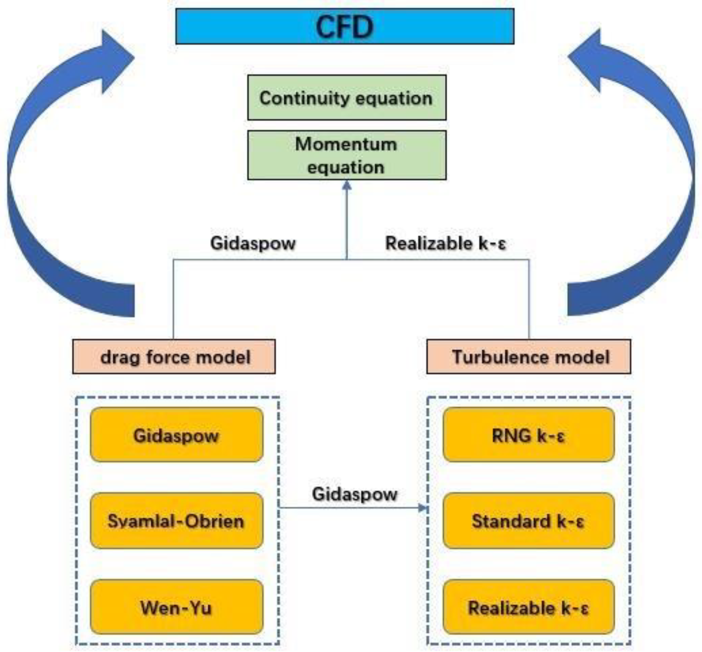
In this study, a commercial CFD software package (Fluent V6.3) was used to simulate the mixing of the anaerobic fermentation tank by solving the conservation of mass and momentum equations. The simulation involved a solid-liquid two-phase system. In these systems, the forces between particles and liquid include drag force, virtual mass force, lift force, diffusive force, etc. Since the lift and virtual mass forces have little influence on the solid phase distribution compared with other forces, the effects of these two forces were ignored in this study. Through comparing the simulation and experimental results, the realizable k-ε model was selected as the turbulence model, and the Gidaspow model was selected as the drag force model. The optimization flow diagram of CFD simulation is shown as Figure 3.
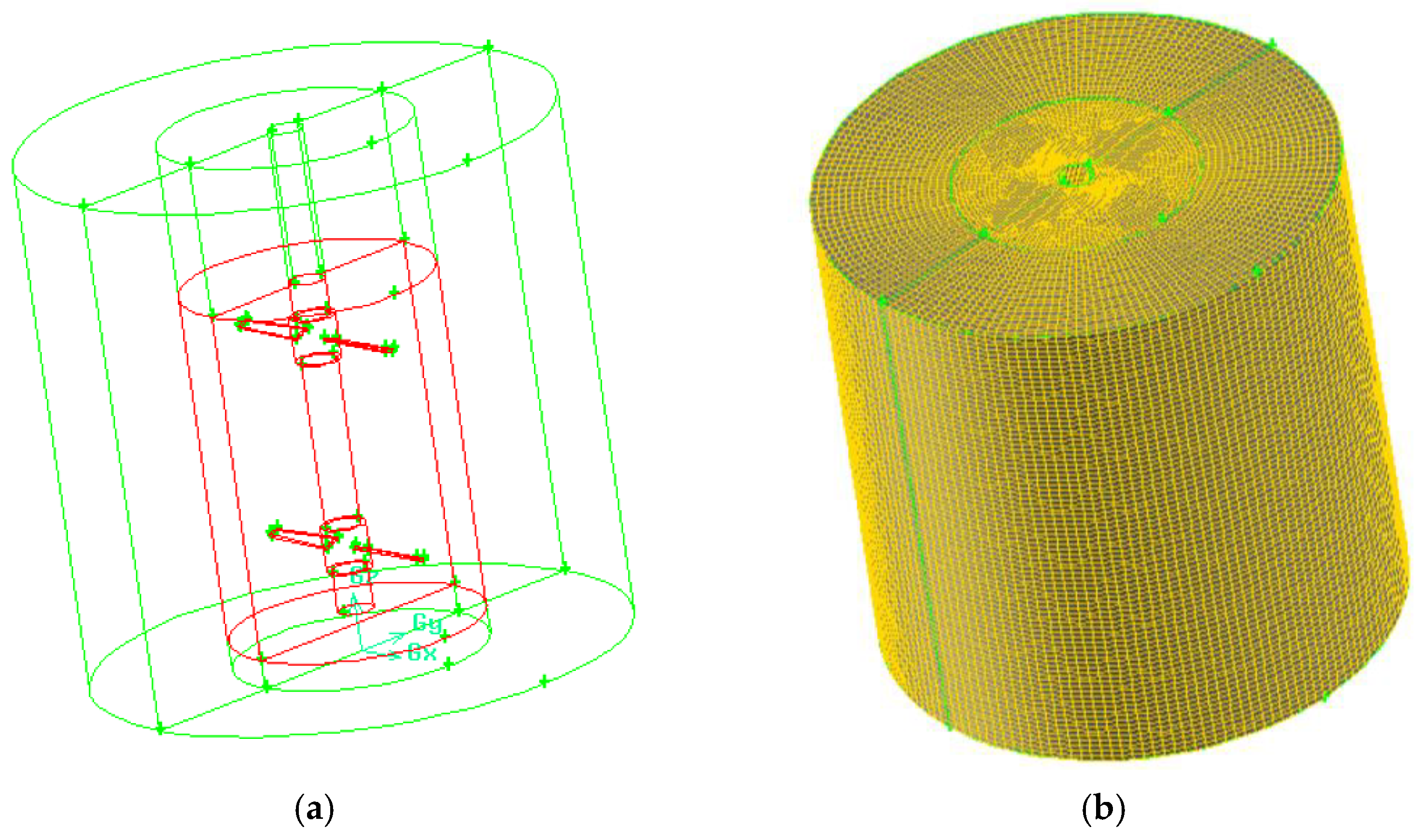
The multiple reference frame (MRF) method [21,22,23] was used to process the computational domain in the simulation. The discrete grids are shown in Figure 4b, using Gambit software, version 2.4, for meshing. The model was divided into a rotational region containing two impellers and an outer stationary region, with mesh sizes adjusted to 2–7 mm, respectively. The total numbers of grids generated were about 1.31 million (lab test) and 2.56 million (pilot test). The stationary region speed was 0 during the simulation, while the rotational region speed was set according to the simulation conditions. Structured meshes were used for the stationary region with a regular shape when meshing. At the same time, unstructured meshes were used for the rotational region with an irregular shape to achieve a trade-off between mesh quality and computing speed. All meshes passed the grid independence check.
The computational domain was divided into a rotational region and a stationary region. The area between the rotational and stationary regions was set as the interface to facilitate material exchange and momentum. The free liquid surface in the tank was set as the symmetry. The inner wall of the stirring tank, blade, and shaft was set as the wall, which could not be used for material exchange.
The finite volume methods discretized the governing equations, including the first-order upwind, second-order upwind, central difference, and QUICK schemes. To improve the calculation accuracy, the second-order upwind scheme was used to discretize the turbulent kinetic energy, momentum, and turbulent dissipation rate. The QUICK scheme was selected to discretize the volume fraction. The simulation run required 12,000–15,000 iterations to converge. The simulation was performed on a 3.0-GHz, 2 GB RAM, Pentium IV. The convergence of the calculation was judged by checking whether the iterative residual error was less than 10−5. At the same time, the solid volume fraction in a section and local area was monitored. When the value did not change while the number of iteration steps increased, it was considered that the simulation had reached a stable state under this condition.
3. Results and Discussion
3.1. Validation and Comparison of Models
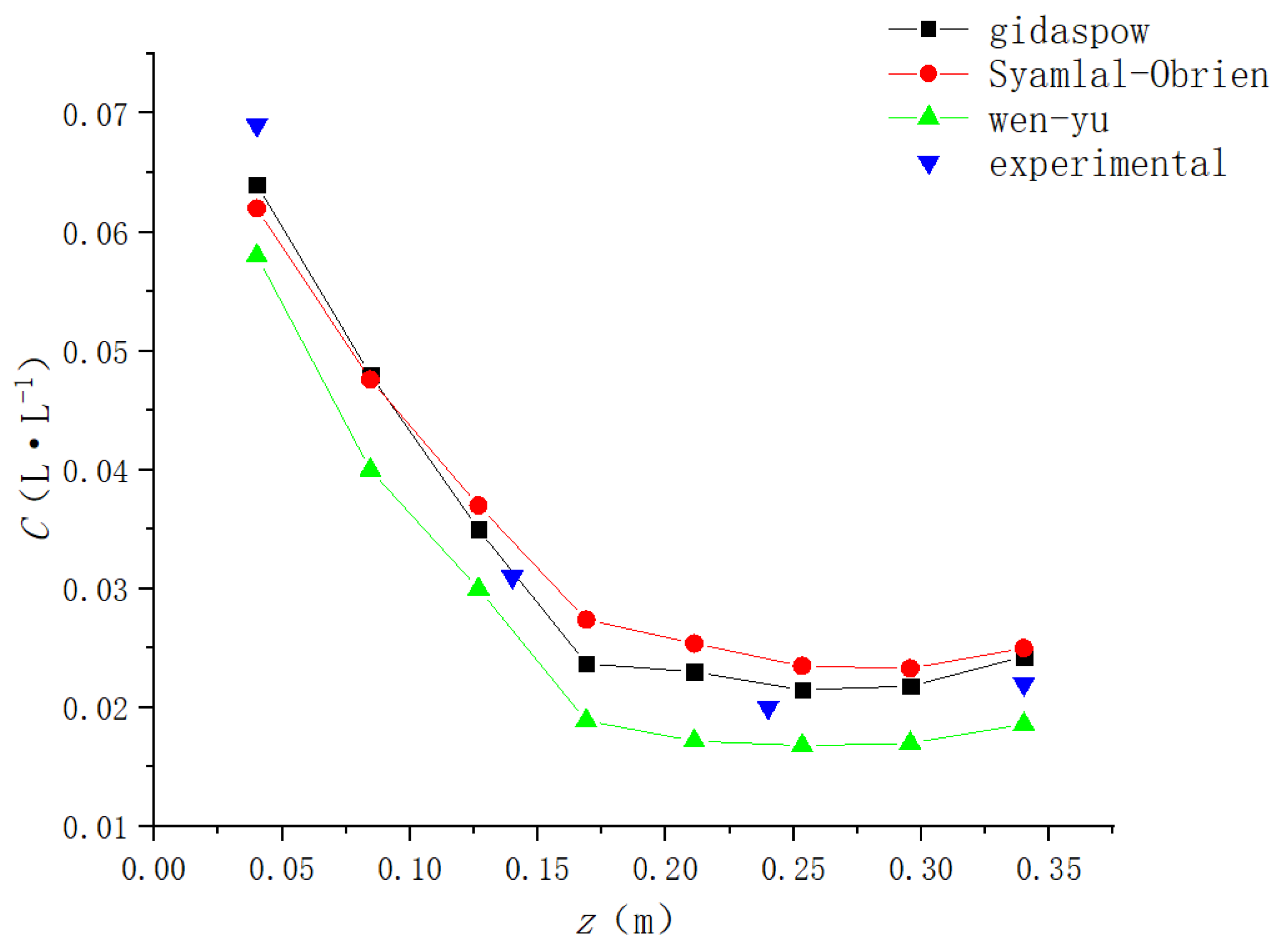
Gidaspow [24], Syamlal-Obrien [25], and Wen-Yu [26] were selected for calculation, and the simulation results were compared with the experimental results, as shown in Figure 5.
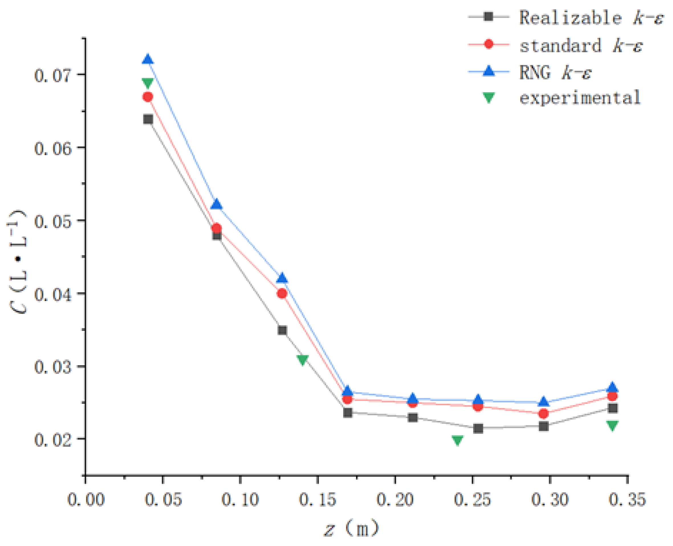
As shown in Figure 5, the axial solid concentration distribution trends under the three drag force models were similar, but the overall values had specific differences. The maximum deviations between the simulated and experimental values of the Gidaspow, Syamlal-Obrien, and Wen-Yu models were 7.24%, 13.63%, and 15.94%, respectively. The Wen-Yu model obtained the lowest concentration, while the Syamlal-Obrien and Gidaspow models obtained similar results. Compared with the experimental results, none of the drag force models could precisely match the experimental values. However, the simulation results of the Gidaspow model were more consistent with the experimental results. Therefore, the Gidaspow model was chosen for this study. Based on the Gidaspow model, turbulence models, such as standard k-ε, realizable k-ε, and RNG k-ε models, were conducted. The comparison between the simulation and the experimental results is shown in Figure 6. The maximum deviations between the simulated and experimental values of the three turbulence models were 17.72%, 7.24%, and 22.72%, respectively.
Figure 6 shows that the axial solid concentration distribution trends under three turbulence models were similar. Among them, the solid concentration calculated by the RNG k-ε model was significantly higher than the experimental value, while the other two were close to the experimental values. Although the RNG k-ε model considers turbulent vortices, the flow situation in the tank is more complex under double-layer impeller stirring. The generated turbulent eddies are not as regular as with the single-layer impeller stirring, which may lead to inaccurate calculation of the RNG k-ε model. The standard k-ε model is widely adaptable and can be applied to most working conditions. It can be observed in Figure 6 that the maximum deviation was less than 20%. The realizable k-ε model had good predictive ability for rotary flows; its simulation results were the closest to the experimental results. Therefore, the realizable k-ε model was selected for simulation.
3.2. Analysis of Scale-Up Criteria
3.2.1. Scale-Up Criterion Based on the Same Blade Tip Linear Velocity
Based on this criterion, the blade tip linear velocity with the mixing equipment in different sizes is equal, which means that the flow velocity at the same fluid position is equal [27]. The criterion can be expressed as follows:
where N is the rotational speed, and D is the diameter of the tank.
Table 3 shows the parameters calculated according to the same blade tip linear velocity. From the definition of unit volume power, it can be expressed as PVN3D2. As show in Table 3, when the blade tip linear velocity was constant, the Reynolds number in the stirring tank rose with the increase in the stirring tank diameter, and the stirring power ratio was the square of the diameter proportion of the tank. At the same time, the power growth speed was accelerated. In the anaerobic fermentation scaling up process, special attention should be paid to the influence of shear force on microbial activity. Nielsen et al. [28] showed that, when the blade tip linear velocity was greater than 3.2 m/s, the shear force may cause damage to microorganisms. The blade tip linear velocity before and after scale-up was the same, so it can be considered that this scale-up criterion had little effect on microbial activity.
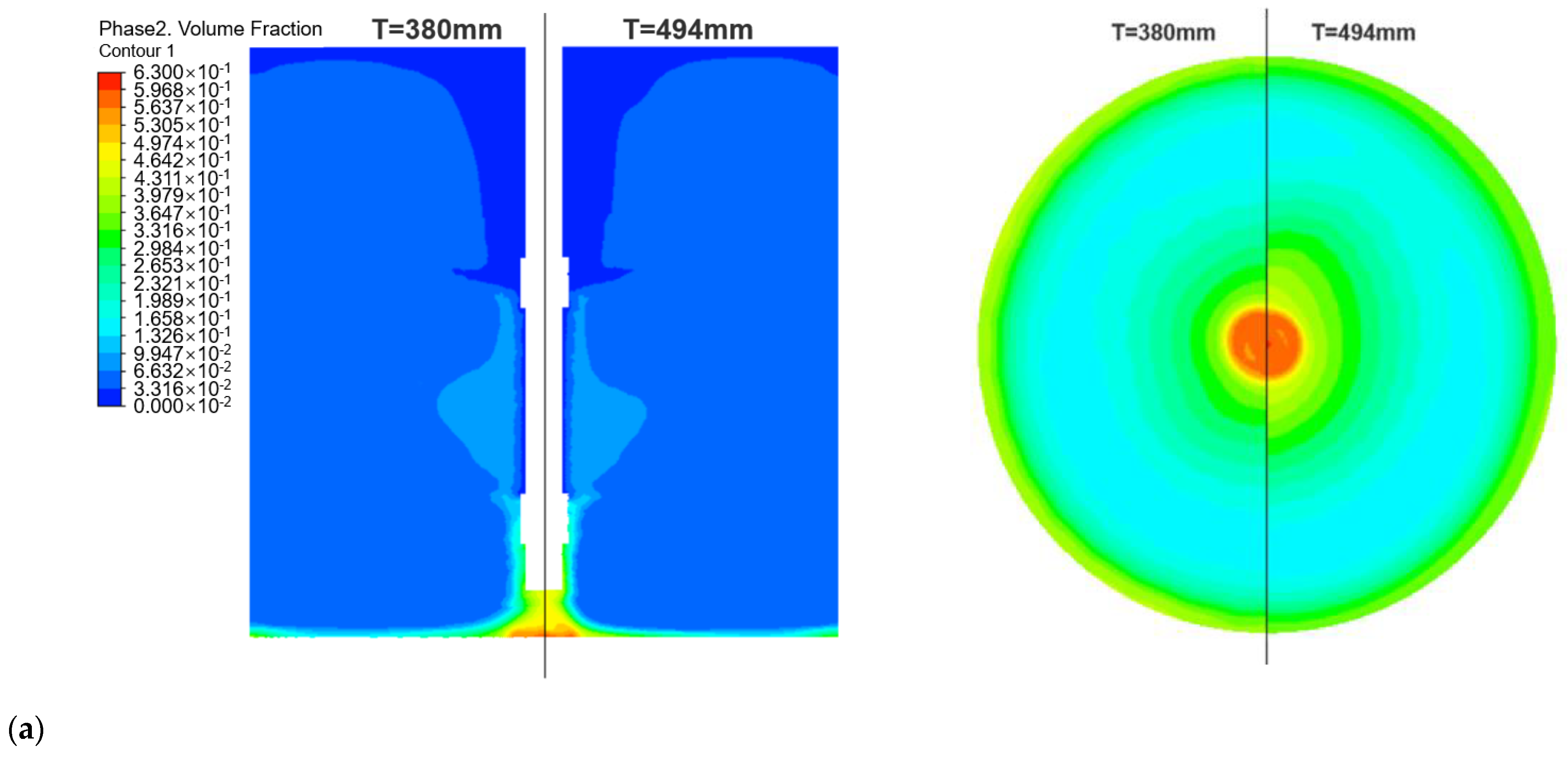
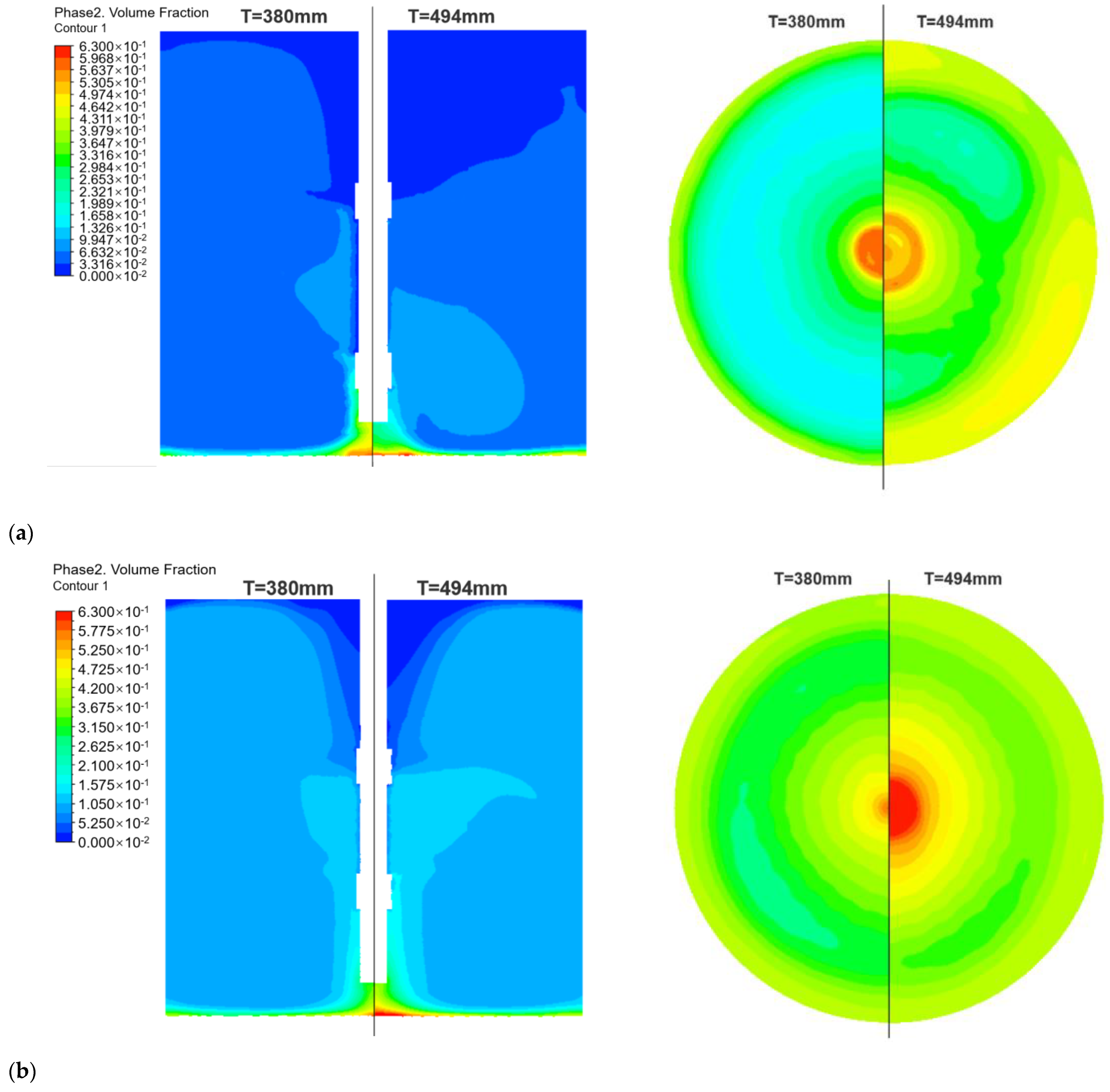
Figure 7 displays the cloud diagrams of the solid concentration distributions under three solid volume fraction conditions scaled up based on the same blade tip linear velocity. The results show that, as the solid volume fraction increased, the solid concentration distribution in the pilot-scale tank compared with the lab-scale tank changed from better to worse. This outcome was consistent with the conclusions drawn by Harrison et al. [13]. Accordingly, the scale-up criterion based on the same blade tip linear velocity could be selected for low solid volume fraction conditions.
To better quantify whether each criterion was applicable to the scale-up processes of anaerobic fermentation reactors with different solid content, the solid uniformity σ was introduced, which can be expressed by the following formula:
where is the local solid phase concentration at the measuring point, and is the average value of the local solid phase concentration at each point.
Table 4 records the solid uniformity σ of the tanks before and after scaling up, according to the same blade tip speed criterion under different solid content. It can also be seen from Table 4 that, when solid content was between 5% and 10%, the σ values of the pilot-scale tank and the lab-scale tank were similar, which means this criterion could be used for the scale-up process under this condition.
3.2.2. Scale-Up Criterion Based on the Same Reynolds Number
The Reynolds number is a dimensionless number used to characterize fluid flow state. For Newtonian fluids, the calculation formula is shown as Equation (7). In stirring equipment, it is generally believed that turbulence is defined when the Reynolds number is higher than 300 under unbaffled conditions. The scale-up criterion derived from the same Reynolds number can be shown in Equation (8):
where N is the rotational speed, and D is the diameter of the tank.
Table 5 lists the parameters calculated according to the same Reynolds number. It can be easily seen that the rotating speed and the blade tip linear velocity decreased after scaling up, as well as the total power and unit volume power. Comparing the calculation results with various scale-up criteria, the rotating speed scaled up based on the same Reynolds number was the lowest. Although the Reynolds number can characterize the flow condition, achieving the same suspension condition with a lower unit volume power is practically impossible, which can also be proved by Figure 8. Generally, the Reynolds number of a large tank is usually higher than that of a small one, so it is impractical to scale up according to the same Reynolds number under actual production conditions. Mishra et al. [29] also presented the same views on this scale-up criterion.
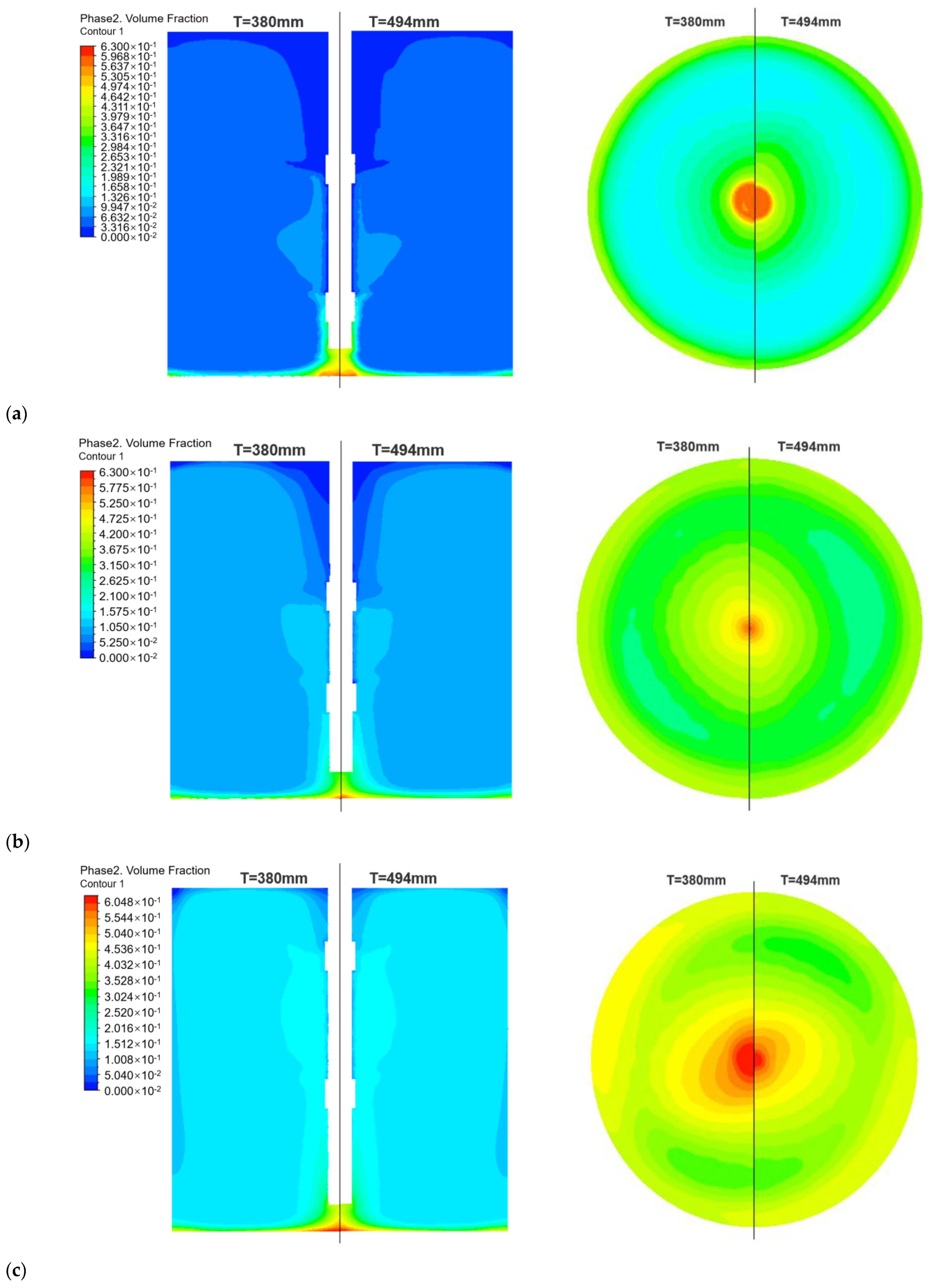
Figure 8 shows the cloud diagrams of the solid concentration distributions under three solid volume fraction conditions scaled up according to the same Reynolds number. Although the Reynolds number characterizes the flow condition to some extent, it can be seen from Figure 8 that, when the Reynolds number is constant, the mixing conditions deteriorate as the scale of the stirring tank increases. As shown in the cloud diagram, there is some solid deposition at the bottom under all three solid volume fraction conditions because the unit volume power decreases rapidly with scaling up according to the same Reynolds number, resulting in the energy system obtained not being able to meet the requirement of uniform solid suspension. In general, although the decrease in blade tip linear velocity based on the same Reynolds number scale-up criterion benefits the survival of microorganisms, the disadvantages caused by the poor solid-liquid mixing effect are far more significant than the former.
Table 6 records the solid uniformity σ of the tanks before and after scaling up, according to the same Reynolds number criterion under different solid content. It can easily be seen from Table 6 that there was a large gap in the σ values before and after scaling up under the three solid content conditions, also confirming the conclusion reached before.
3.2.3. Scale-Up Criterion Based on the Same Weber Number
The Weber number is also a dimensionless number in fluid mechanics, characterizing the ratio of inertial force to surface tension. The scale-up criterion based on the same Weber number is generally used in liquid–liquid mixing conditions. However, considering this study involved multiple solid volume fractions and the density of solid–liquid phases were relatively close, it was also investigated here. The Weber number can be expressed as Equation (9):
where σ is the surface tension coefficient of the fluid.
The scale-up criterion based on the same Weber number can be further obtained as follows:
Table 7 lists the parameters calculated according to the same Weber number. The results show that the blade tip linear velocity and unit volume power decreased while the Reynolds number and total power increased after scaling up. For anaerobic fermentation systems, the decrease in blade tip linear velocity is beneficial to maintain microbial activity. Therefore, the negative impact of blade tip linear velocity on microorganisms in scaling up processes can be ignored by selecting the scale-up criterion with the same Weber number.
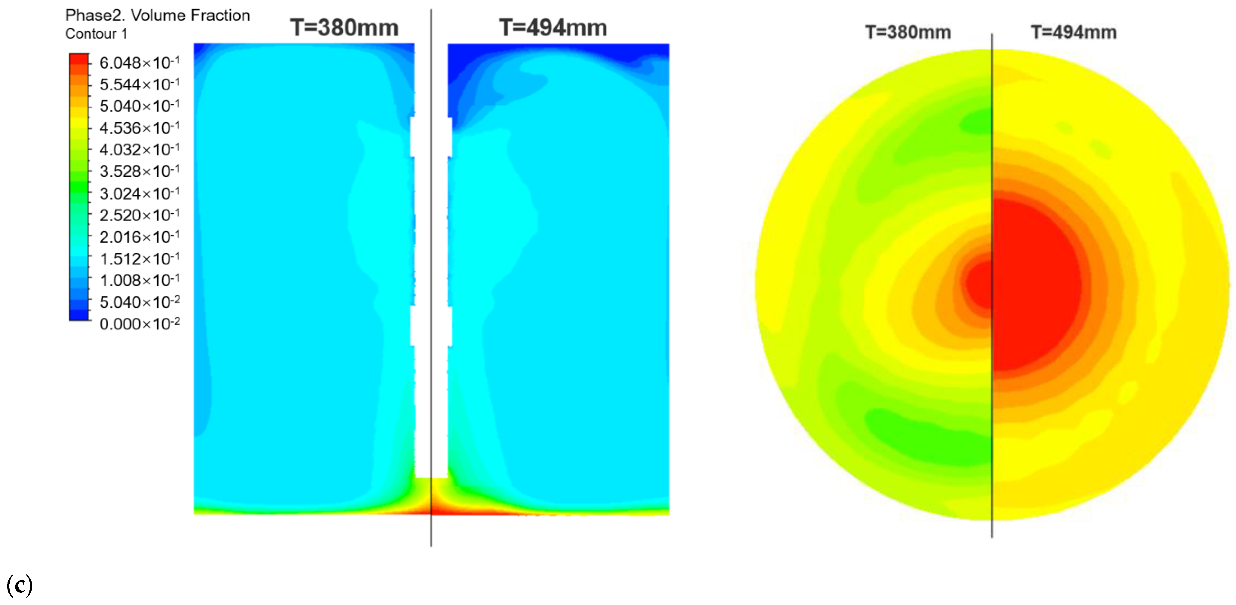
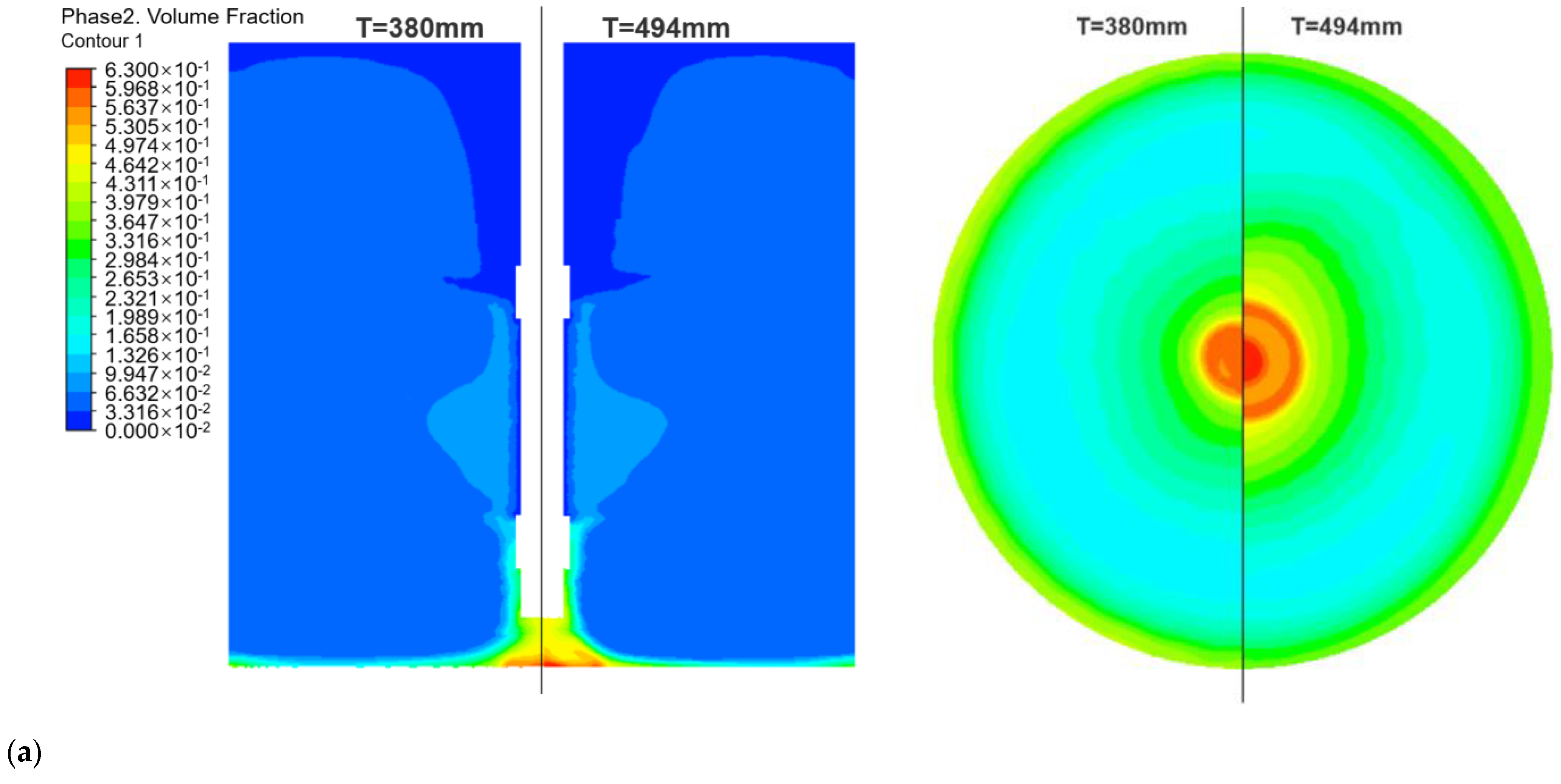
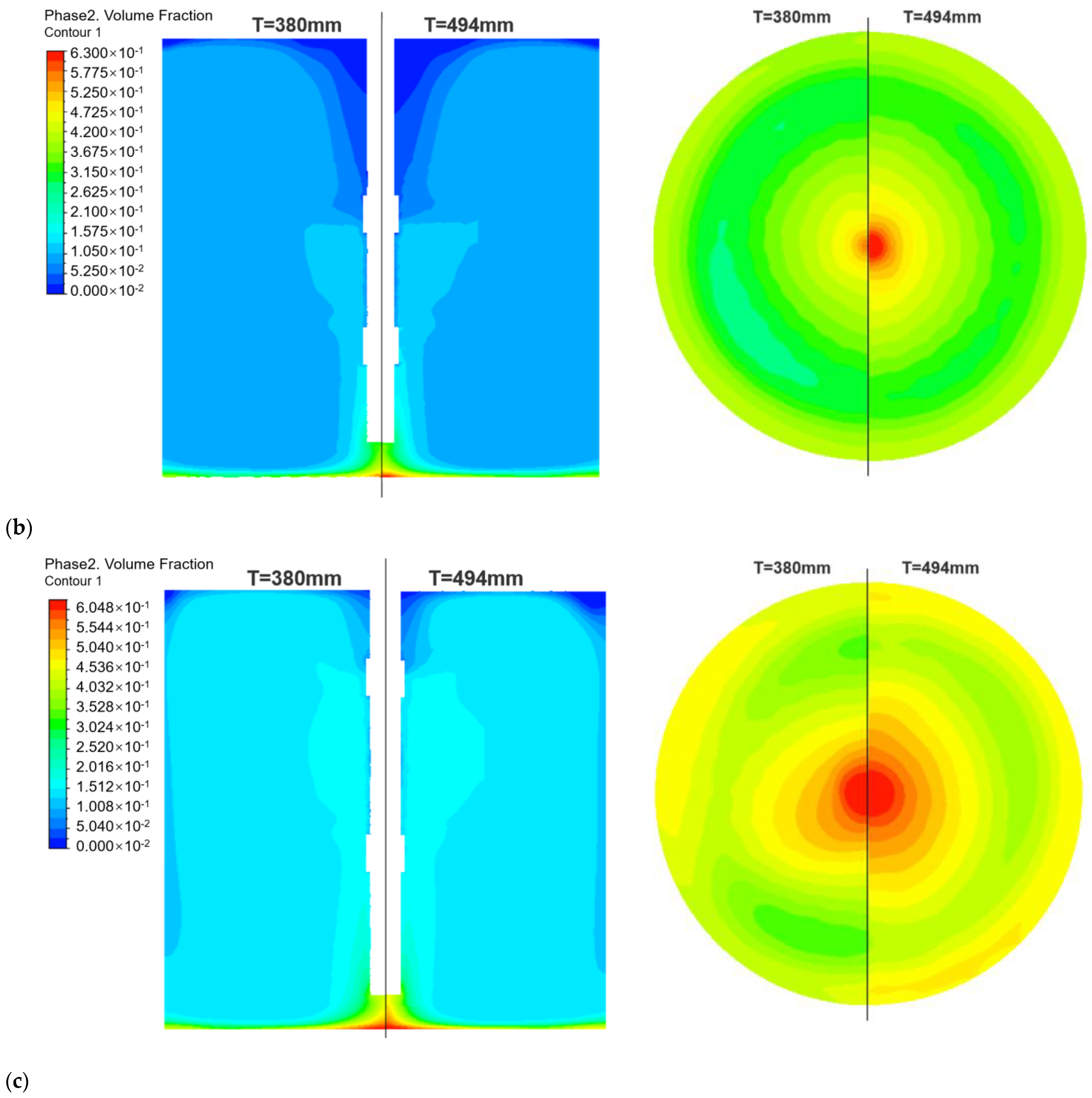
Figure 9 shows the cloud diagrams of the solid concentration distributions under three solid volume fraction conditions scaled up according to the same Weber number. It can be seen from Figure 9 that, when the solid volume fraction was 5% v/v and 10% v/v, the solid concentration distribution was more similar between the pilot-scale and lab-scale tanks because, when the density of the solid and liquid phases is relatively close in anaerobic fermentation systems, the scaling up process can be simplified to pure liquid phase scale-up under a low solid volume fraction condition. With the increase in the solid volume fraction, the density difference between the solid and liquid phases and the force between the particle–particle, particle–wall, and solid–liquid phases cannot be ignored. When the solid volume fraction reached 15% v/v, the reproducibility of the solid concentration distribution was worse than that of 5% v/v and 10% v/v.
Table 8 records the solid uniformity σ of the tanks before and after scaling up, according to the same Weber number criterion under different solid content. As can be seen from Table 8, with the increase in solid content, the gap of solid uniformity in the tanks became larger before and after scaling up. Therefore, this scale-up criterion is only applicable to anaerobic fermentation mixing systems with a solid content of less than 5%.
3.2.4. Scale-Up Criterion Based on the Same Unit Volume Power
Unit volume power is the energy used to stir per unit of fluid volume per unit of time [30]. In scaling up processes, the scale-up criterion based on the same unit volume power is shown in Equation (11):
Table 9 lists the parameters calculated according to the same unit volume power. The results show that the blade tip linear velocity, unit volume power, and total power increased after scaling up. Although this scale-up criterion is commonly used, it is necessary to consider whether the blade tip linear velocity will affect microbial reactions for stirring equipment with cells or microorganisms. It can be calculated that, when the volume of the stirring tank is enlarged by eight times, the maximum blade tip linear velocity reaches 3.01 m/s, and further enlargement will cause adverse effects on microbial activity. Generally, considering the influence of the blade tip linear velocity, some bioreactors will choose the same blade tip linear velocity as the scale-up criterion [31]. For conditions without considering this factor, better mixing results can be obtained by scaling up with the same unit volume power, rather than scaling up based on the same blade tip linear velocity.
Figure 10 shows the cloud diagrams of the solid concentration distributions under three solid volume fraction conditions scaled up according to the same unit volume power. It can be seen from Figure 10 that, under this scale-up criterion, the solid concentration distribution of the pilot-scale tank was better compared with the lab-scale one because only the mechanical components, such as the tank body, shaft, and blades, are scaled up in the scaling up process of the stirring equipment, while the particle size of the solid phase remains the same. In other words, the pilot-scale tank stirs smaller particles at the same unit volume power as the lab-scale tank. The small particle size is more accessible to suspend than the large particle size [32]. Therefore, selecting the scale-up criterion based on the same unit volume power for solid-liquid mixing will cause energy waste when the physical properties of the solid and liquid phases are unchanged.
Table 10 records the solid uniformity σ of the tanks before and after scaling up, according to the same unit volume power criterion under different solid content. As shown in Table 10, under the three solid content conditions, the values of σ of the lab-scale tank were always greater than those of the pilot-scale tank, confirming the conclusion obtained from the cloud diagrams that the solid uniformity is better after scaling up according to this criterion.
3.2.5. Scale-Up Criterion Based on the Same Solid Suspension Degree
According to the different purposes of operation, the degree of solid suspension can be divided into two states. One is the critical suspension state, which means that the solid particles stay at the bottom of the stirring tank for no more than 2 s, but the solid particles are not homogeneously suspended. The other is the homogeneous suspension state, which means that the solid particles in the tank are evenly distributed throughout the tank. The scale-up criterion based on the same solid suspension degree is shown in Equation (12):
Table 11 lists the parameters calculated according to the same solid suspension degree. The results show that the blade tip linear velocity, Reynolds number, and total power increased while the unit volume power decreased after scaling up. Compared to the scale-up criterion with the same unit volume power, the blade tip linear velocity increased much slower using the former scale-up criterion, which is beneficial to bioreactors.
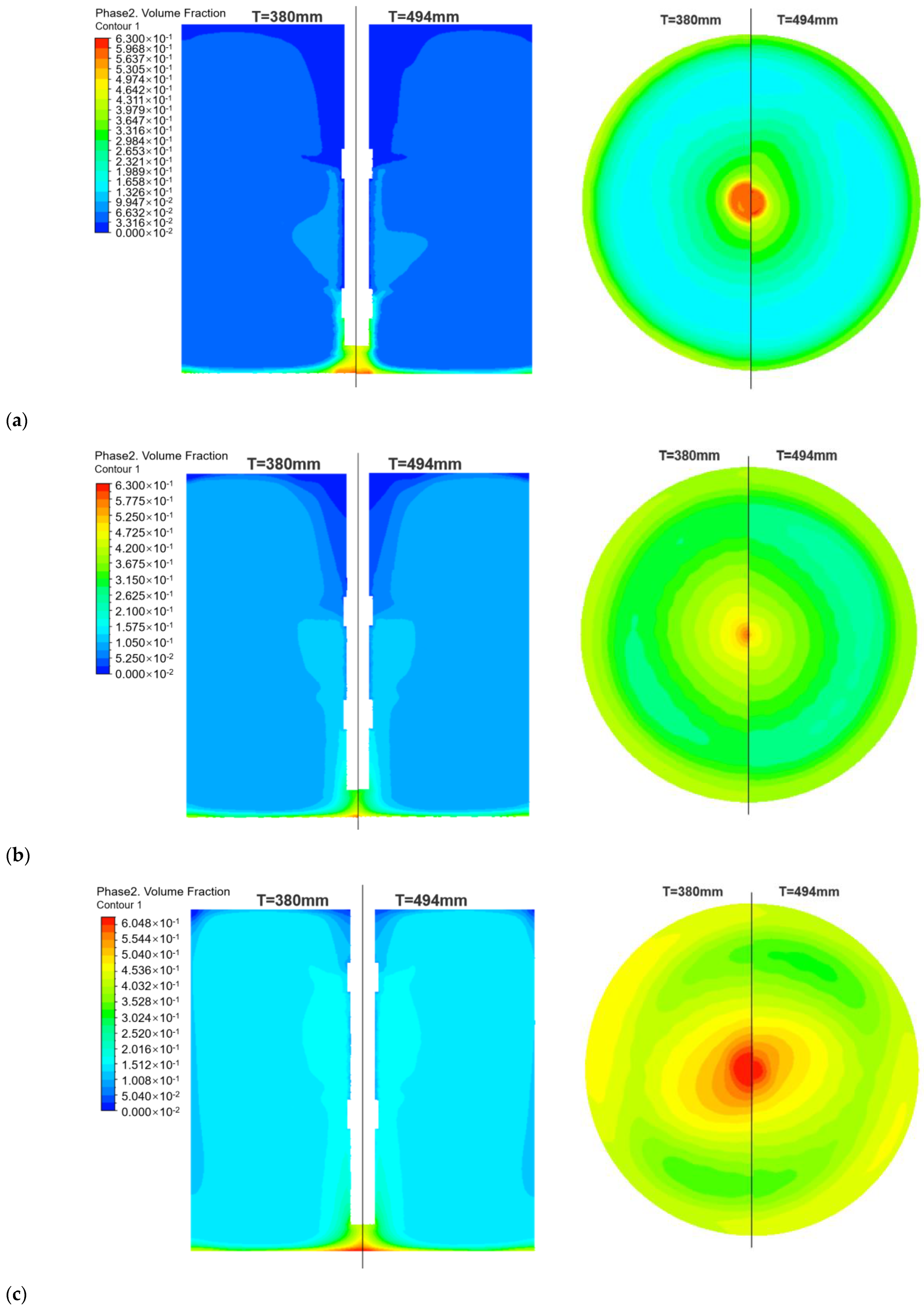
Figure 11 shows the cloud diagrams of the solid concentration distribution under three solid volume fraction conditions scaled up according to the same solid suspension degree. It can be seen from Figure 11 that the solid concentration distributions were similar, respectively scaled up with the same solid suspension degree and the same unit volume power. Although the scale-up index of 0.75 according to the same solid suspension degree had been empirically determined by experts, it can be seen in Figure 11 that the solid suspension degree before and after scaling up was not precisely the same. Therefore, during the scaling up of anaerobic fermentation mixing equipment, it is necessary to conduct the corresponding scale-up design according to the specific conditions.
Table 12 records the solid uniformity σ of the tanks before and after scaling up, according to the same solid suspension degree criterion under different solid content. Since the impeller speeds in the two scale-up situations were similar, the σ values in the tanks were basically the same when scaled up based on the same unit volume power and the same solid suspension degree. It can be basically considered that the best mixing effect can be satisfied when the scale-up index is 0.75, and there is no need to further reduce it. If the solid phase concentration distribution has high requirements, it can be directly selected to scale up according to the same solid suspension degree criterion.
3.3. Optimization of Scale-Up Criteria for Different Solid Content Systems
To select the scale-up criteria suitable for different solid content more accurately, we considered 36 measuring points on one side of the stirring tank. The ratios between the point locations (ri) and the stirring tank radius (R) in the radial direction were r1/R = 0.2, r2/R = 0.4, r3/R = 0.6, and r4/R = 0.8, respectively. The longitudinal range of points was 0.1~0.9 H from the bottom of the tank, including nine measuring points equidistantly taken from the remaining areas. Since the cloud diagrams of the solid concentration distribution scaled up with different scale-up criteria are given above, they are not repeated here. To quantify the solid-liquid mixing condition, the mixing index (MI) was used to quantitatively characterize the uniformity of the solid concentration distribution in the tank. The definition formulas are as follows:
where Xi (i = 1,2, 3…, n) is the relative solid concentration at each measuring point, is the mean value of the relative solid concentration at all measuring points, and n is the number of measuring points in the selected plane.
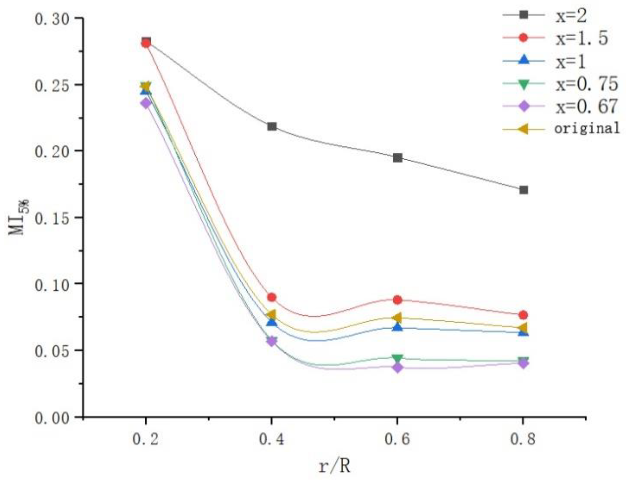
Figure 12, Figure 13 and Figure 14 show the influence of different scale-up criteria on the MI curve with three solid volume fraction conditions. The data for each radial position (ri/R) were the mean of the longitudinal values. The original MI curve characterizes the mixing condition in the original tank. According to Figure 12, Figure 13 and Figure 14, the mixing index decreased and tended to be stable with the decrease in the distance from the wall, indicating that the axial concentration gradient in the near-wall region is small. It can also be seen from the previous concentration distribution cloud diagrams that it was related to the axial and radial flows generated by the two-pitched blade impellers.
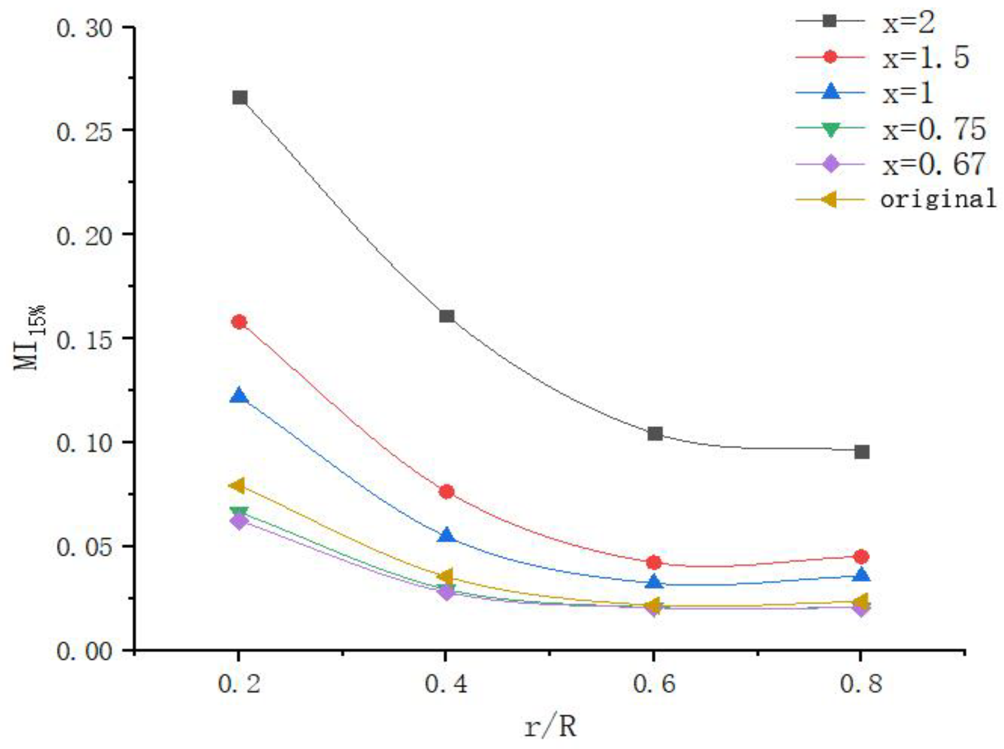
At the same time, it is found that, as the solid volume fraction increased, the scale-up index corresponding to the curve similar to the original MI curve became smaller. For the 5% solid volume fraction system, the original MI curve was between the curves belonging to the scale-up indices of 1 and 1.5. For the 10% solid volume fraction system, the original MI curve and the curve belonging to the scale-up index of 1 almost overlapped. Regarding the 15% solid volume fraction system, the original MI curve was between the curves belonging to the scale-up indices of 0.67 and 1. This result is sufficient to demonstrate the effect of the solid volume fraction on the scaling up of solid–liquid stirring equipment.
In addition, Figure 12, Figure 13 and Figure 14 show that, with the increase in the solid volume fraction, the MI curves with scale-up indices of 0.75 and 0.67 become closer. It can be considered that, even if the solid volume fraction continues to increase, using the scale-up index of 0.75 can already achieve the same mixing effect in the scaling up process. Additionally, this condition is the most uniform condition that can be achieved in actual production.
To better reproduce the solid distribution of the original tank, the scale-up index under different solid content conditions was optimized. The scale-up index range in which the MI curve was closer to the original tank curve was taken as the optimization range. According to Figure 12, the optimization range of the scale-up index under a 5% solid volume fraction was positioned from 1 to 1.5. The solid concentration distribution was simulated with the scale-up indices of 1.1, 1.2, 1.3, and 1.4, respectively. Similarly, the optimization range was positioned from 1 to 1.5 under a 10% solid volume fraction in Figure 13. The simulation process was the same as previously mentioned. According to Figure 14, the optimization range was positioned from 0.75 to 1 under a 15% solid volume fraction. The solid concentration distribution was simulated with scale-up indices of 0.8, 0.85, 0.9, and 0.95, respectively.
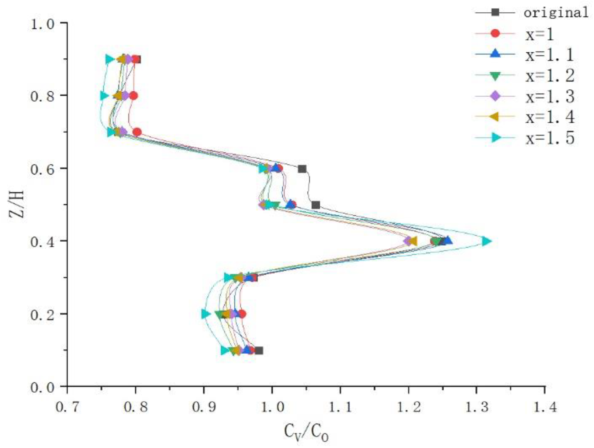
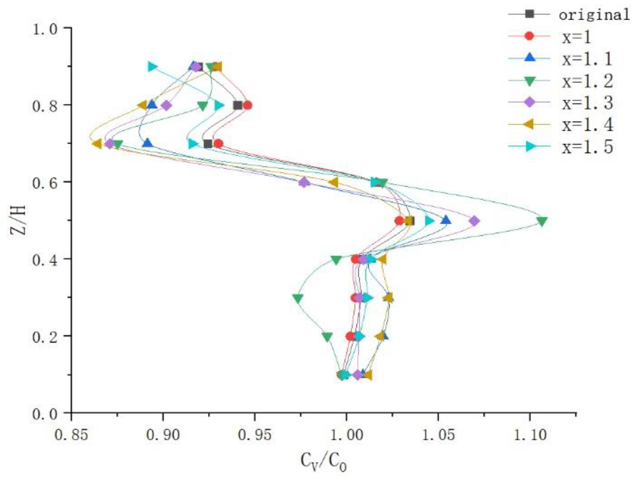
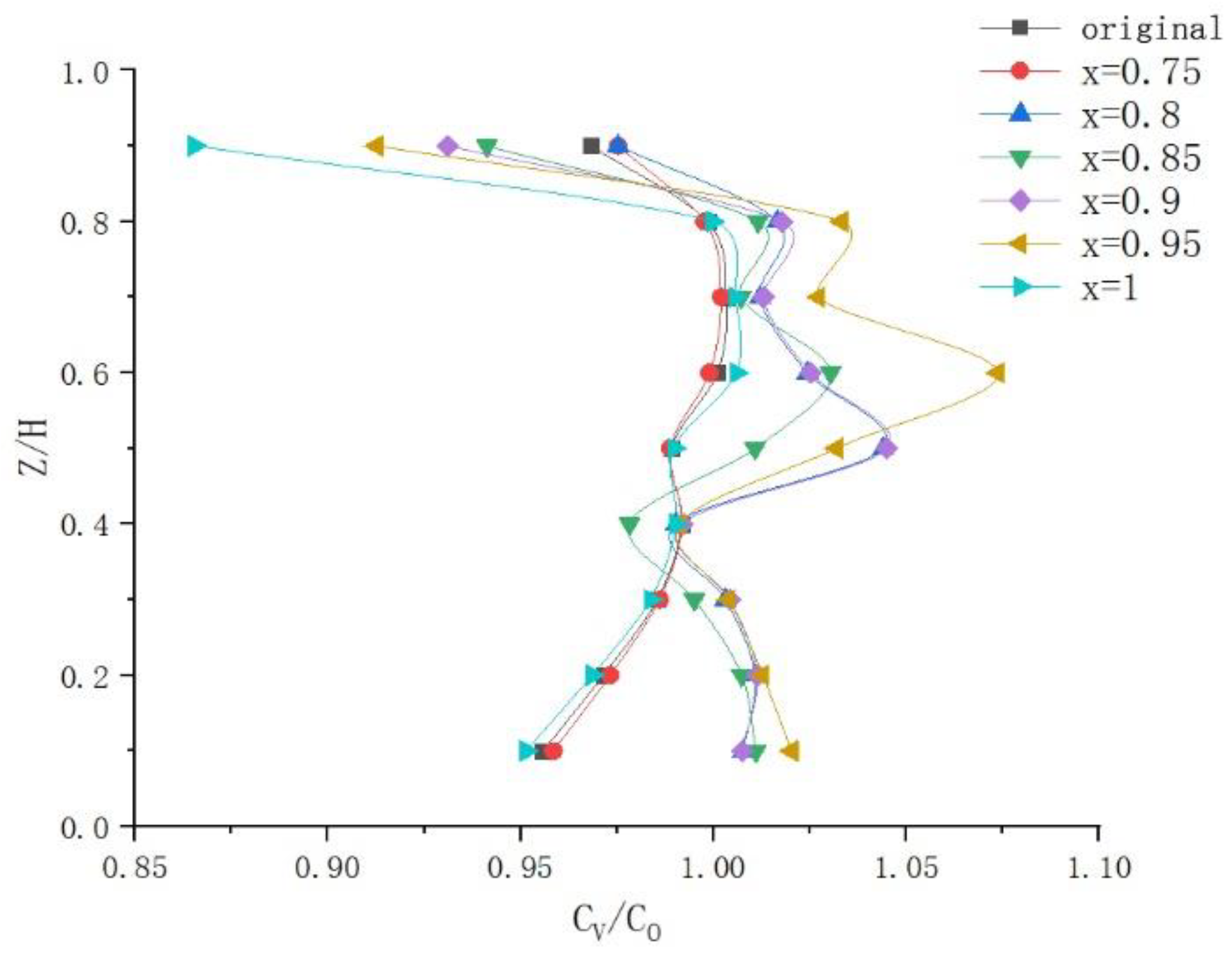
Figure 12, Figure 13 and Figure 14 show that the mixing index was lower near the tank wall. The difference between the mixing index of the stirring equipment scaled up under different criteria was relatively minor near the wall. Therefore, in the further comparison of solid concentration distributions, we chose the part close to the stirring axis for comparison. However, the mixing effect at r/R = 0.2 was not globally representative due to the large gap between the mixing condition here and that at other positions. Finally, the solid concentration distribution at r/R = 0.4 was selected as the basis for optimization. Figure 15, Figure 16 and Figure 17 show the axial concentration distributions of 5%, 10%, and 15% solid volume fraction, respectively, under different scale-up indices.
The maximum relative deviation between the axial concentration distribution curve of the stirring tank after scaling up and that of the original tank curve was used as the benchmark to judge the reproduction effect. The details of the operations are explained in the following steps:
Step 1: The solid concentration of nine axial points at r/R = 0.4 in simulation results were derived;
Step 2: The relative deviation of the axial concentration distribution between the stirring equipment after scaling up and the original tank was calculated. The maximum value of the relative deviation under each scale-up index was recorded;
Step 3: Finally, by comparing the maximum relative deviation under each scale-up index, the minimum result was selected, and the corresponding scale-up index was identified as the optimized scale-up index.
According to the calculation results, the optimized scale-up indices were 1.1, 1, and 0.75, respectively, at 5%, 10%, and 15% solid volume fractions, and the corresponding maximum relative deviations were 3.64%, 0.98%, and 0.73%, respectively. It can be concluded that a system with a higher solid concentration requires a smaller scale-up index to reproduce the same mixing conditions. This conclusion is consistent with the research results of Harrison et al. [13].
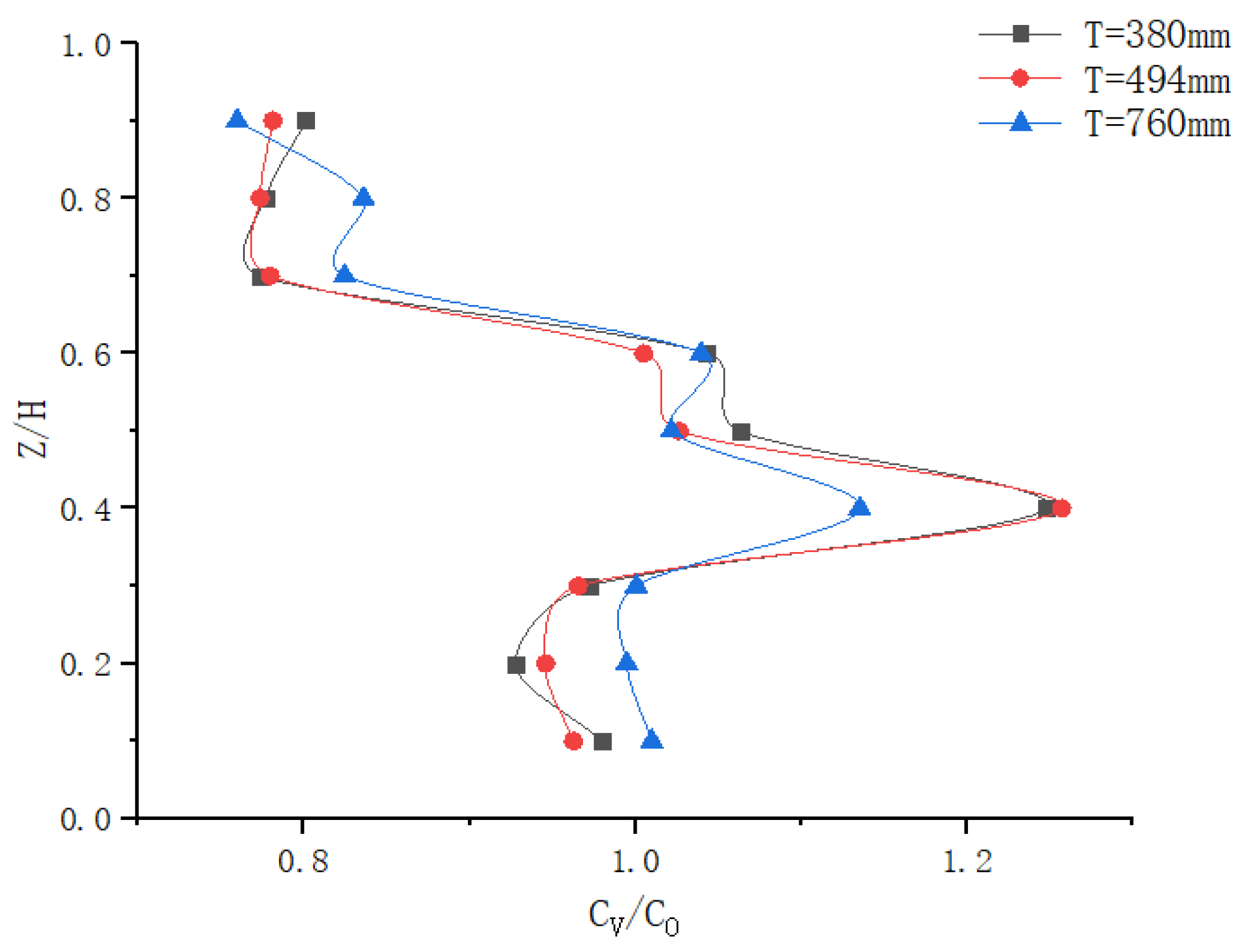
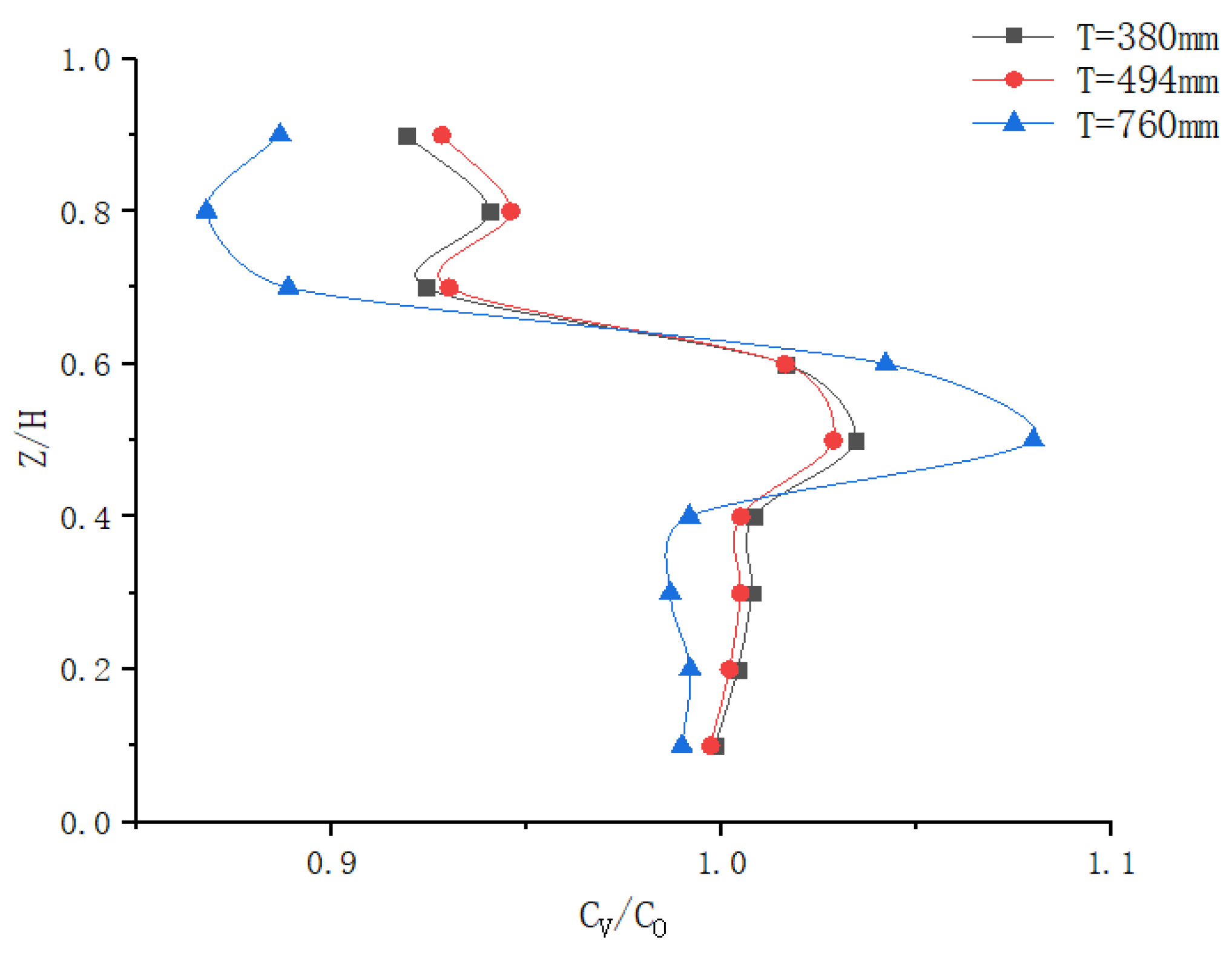
Based on the optimization of the scale-up indices under three solid content conditions mentioned above, the anaerobic fermentation reactor was further enlarged, and the solid phase concentration distribution in the three scales of tanks was selected to verify the reliability of the optimized scale-up indices. The structural parameters of the three scales of tanks (including the lab-scale and pilot-scale tanks) are shown in Table 13.
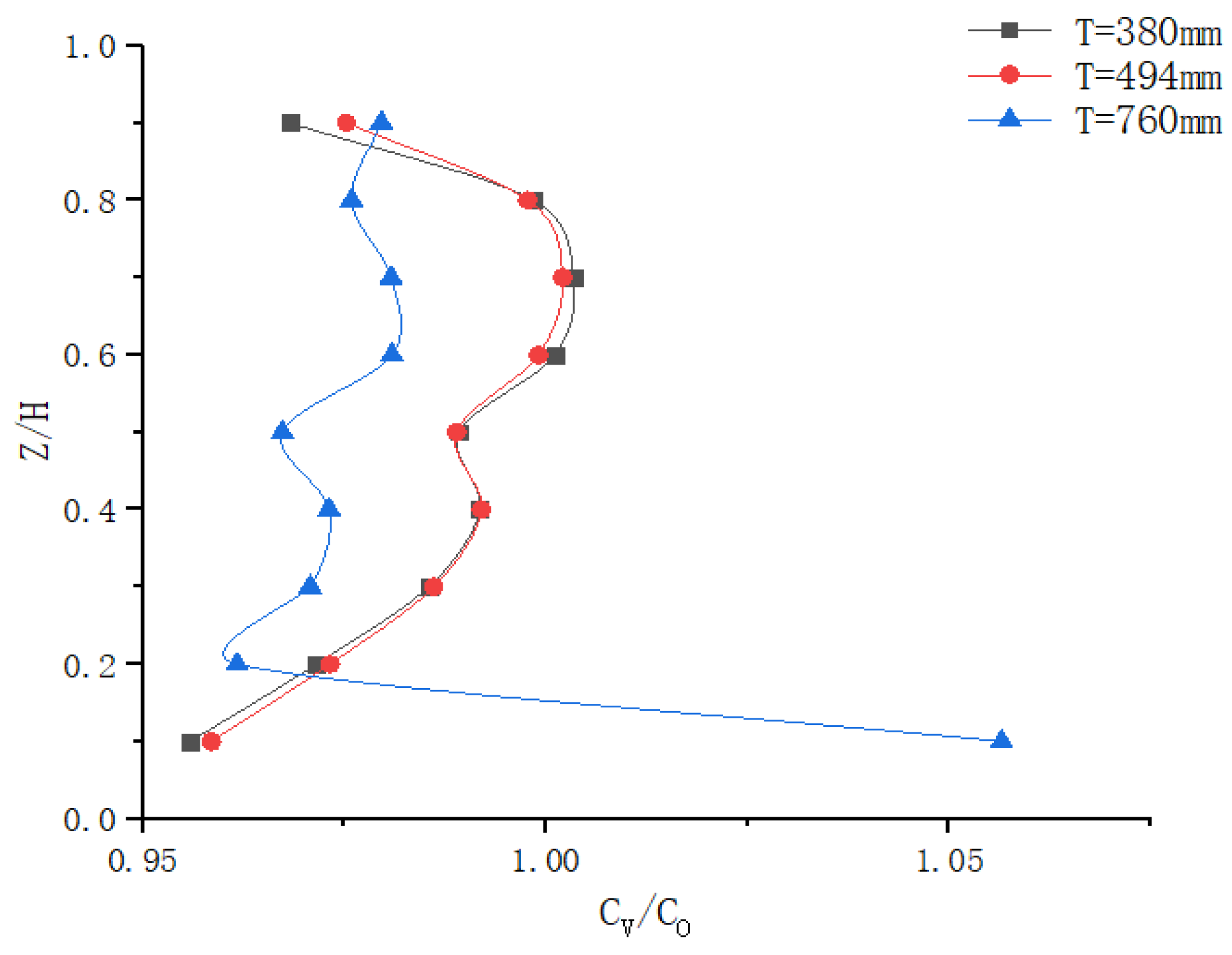
Figure 18, Figure 19 and Figure 20 show the solid concentration distributions at r/R = 0.4 during the scale-up process under three solid content conditions. The maximum relative deviations of large and lab tests were 6.6%, 7.73%, and 10.52%, respectively. The solid concentration distribution of the large test was similar to that of the lab and pilot tests, indicating that the reproduction was good.
4. Conclusions
The geometric similarity method was used to scale up anaerobic fermentation stirring equipment. The applicability of different scale-up criteria was analyzed by investigating the relative parameters. On this basis, the scale-up index was optimized and verified. The Weber number criterion applied to a less than 5% solid content system. The blade tip speed criterion applied to a 5% to 10% solid content system, which was especially suitable for conditions that limit the shear rate, such as straw anaerobic fermentation. The Reynolds number criterion was not recommended due to the poor mixing effect. When the scale-up index x reached 0.75, there was no need to further reduce it. For anaerobic fermentation systems, the suitable scale-up indices selected for 5%, 10%, and 15% solid content were 1.1, 1, and 0.75, respectively.
Author Contributions
Conceptualization, Z.L. and Z.Z.; methodology, H.L.; software, Z.L.; validation, Z.L., Z.Z. and H.L.; investigation, Z.L. and H.L.; resources, Z.L. and H.L.; data curation, Z.L. and Z.Z.; writing—original draft preparation, Z.L.; writing—review and editing, Z.L. and Z.Z.; visualization, H.L. and Z.Z.; supervision, B.L.; funding acquisition, B.L. All authors have read and agreed to the published version of the manuscript.
Funding
This research was funded by the National Natural Science Foundation of China (grant numbers 21978255 and 21776246).
Institutional Review Board Statement
Not applicable.
Informed Consent Statement
Not applicable.
Data Availability Statement
Data reported in this study are contained within the article. The underlying raw data are available on request from the corresponding author.
Conflicts of Interest
The funders had no role in the design of the study; in the collection, analyses, or interpretation of the data; in the writing of the manuscript; or in the decision to publish the results.
References
- Braguglia, C.M.; Gallipoli, A.; Gianico, A.; Pagliaccia, P. Anaerobic Bioconversion of Food Waste into Energy: A Critical Review. Bioresour. Technol. 2018, 248, 37–56. [Google Scholar] [CrossRef]
- Yu, Q.; Liu, R.H.; Li, K.; Ma, R.J. A Review of Crop Straw Pretreatment Methods for Biogas Production by Anaerobic Digestion in China. Renew. Sustain. Energy Rev. 2019, 107, 51–58. [Google Scholar] [CrossRef]
- Paudel, S.R.; Banjara, S.P.; Choi, O.K.; Park, K.Y.; Kim, Y.M.; Lee, J.W. Pretreatment of Agricultural Biomass for Anaerobic Digestion: Current State and Challenges. Bioresour. Technol. 2017, 245, 1194–1205. [Google Scholar] [CrossRef] [PubMed]
- Huang, Y.K.; Dehkordy, F.M.; Li, Y.; Emadi, S.; Bagtzoglou, A.; Li, B.K. Enhancing Anaerobic Fermentation Performance Through Eccentrically Stirred Mixing: Experimental and Modeling Methodology. Chem. Eng. J. 2018, 334, 1383–1391. [Google Scholar] [CrossRef]
- Clark, I.C.; Zhang, R.H.; Upadhyaya, S.K. The Effect of Low Pressure and Mixing on Biological Hydrogen Production via Anaerobic Fermentation. Int. J. Hydrogen Energy 2012, 37, 11504–11513. [Google Scholar] [CrossRef]
- Mcmahon, K.D.; Stroot, P.G.; Mackie, R.I.; Lutgarde, R. Anaerobic codigestion of municipal solid waste and biosolids under various mixing conditions—II: Microbial population dynamics. Water Res. 2001, 35, 1817–1827. [Google Scholar] [CrossRef]
- Gómez, X.; Cuetos, M.J.; Cara, J.; Morán, A.; García, A.I. Anaerobic co-digestion of primary sludge and the fruit and vegetable fraction of the municipal solid wastes. Renew. Energ. 2006, 31, 2017–2024. [Google Scholar] [CrossRef]
- Agfunder. Available online: https://agfundernews.com/synonym-bio-report-documents-global-gaps-in-fermentation-capacity (accessed on 13 February 2023).
- Bhm, L.; Hohl, L.; Bliatsiou, C.; Kraume, M. Multiphase Stirred Tank Bioreactors–New Geometrical Concepts and Scale-up Approaches. Chem. Ing. Technol. 2019, 91, 1724–1746. [Google Scholar] [CrossRef]
- Paul, E.L.; Atiemo-Obeng, V.A.; Kresta, S.M. Handbook of Industrial Mixing: Science and Practice; Wiley: New York, NY, USA, 2004. [Google Scholar]
- Montante, G.; Bourne, J.R.; Magelli, F. Scale-up of Solids Distribution in Slurry, Stirred Vessels Based on Turbulence Intermittency. Ind. Eng. Chem. Res. 2008, 47, 3438–3443. [Google Scholar] [CrossRef]
- Zhou, X.; Liu, Y.; Wen, Y.; Cheng, S.; Yin, J.Z. Simulation of Solid-Liquid Suspension and Scale-up Of Agarose Gel Activation Reactor. J. Mech. Med. Biol. 2016, 16, 1650087. [Google Scholar] [CrossRef]
- Harrison, S.; Kotsiopoulos, A.; Stevenson, R.; Cilliers, J.J. Mixing Indices Allow Scale-up of Stirred Tank Slurry Reactor Conditions for Equivalent Homogeneity. Chem. Eng. Res. Des. 2019, 153, 865–874. [Google Scholar] [CrossRef]
- Jafari, R.; Tanguy, P.A.; Chaouki, J. Experimental Investigation on Solid Dispersion, Power Consumption and Scale-up in Moderate to Dense Solid–Liquid Suspensions. Chem. Eng. Res. Des. 2012, 90, 201–212. [Google Scholar] [CrossRef]
- Buurman, C.; Resoort, G.; Plaschkes, A. Scaling-up Rules for Solids Suspension in Stirred Vessels. Chem. Eng. Sci. 1986, 41, 2865–2871. [Google Scholar] [CrossRef]
- Kuzmani, N.; Aneti, R.; Akrap, M. Impact of floating suspended solids on the homogenisation of the liquid phase in dual-impeller agitated vessel. Chem. Eng. Process. 2008, 47, 663–669. [Google Scholar] [CrossRef]
- Gu, D.Y.; Liu, Z.H.; Xu, C.L.; Li, J.; Tao, C.Y.; Wang, Y.D. Solid-Liquid Mixing Performance in a Stirred Tank with a Double Punched Rigid-Flexible Impeller Coupled with a Chaotic Motor. Chem. Eng. Process. 2017, 118, 37–46. [Google Scholar] [CrossRef]
- Gui, M.; Liu, Z.H.; Liao, B.; Wang, T.; Wang, Y.; Sui, Z.Q.; Bi, Q.C.; Wang, J. Void Fraction Measurements of Steam–Water Two-phase Flow in Vertical Rod Bundle: Comparison among Different Techniques. Exp. Therm. Fluid Sci. 2019, 109, 109881. [Google Scholar] [CrossRef]
- Pjontek, D.; Parisien, V.; Macchi, A. Bubble Characteristics Measured Using a Monofibre Optical Probe in a Bubble Column and Freeboard Region Under High Gas Holdup Conditions. Chem. Eng. Sci. 2014, 111, 153–169. [Google Scholar] [CrossRef]
- Zhang, H.; Johnston, P.M.; Zhu, X.; Lasa, H.I.; Bergougnou, M.A. A novel calibration procedure for a fiber optic solids concentration probe. Power Technol. 1998, 100, 260–272. [Google Scholar] [CrossRef]
- Dong, L.; Johansen, S.T.; Engh, T.A. Flow Induced by an Impeller in an Unbaffled Tank—II. Numerical Modelling. Chem. Eng. Sci. 1994, 49, 3511–3518. [Google Scholar] [CrossRef]
- Harvey, A.D.; Wood, S.P.; Leng, D.E. Experimental and Computational Study of Multiple Impeller Flows. Chem. Eng. Sci. 1997, 52, 1479–1491. [Google Scholar] [CrossRef]
- Naude, I.; Xuereb, C.; Bertrand, J. Direct Prediction of the Flows Induced by a Propeller in an Agitated Vessel Using an Unstructured Mesh. Cana. J. Chem. Eng. 1998, 76, 631–640. [Google Scholar] [CrossRef]
- Ding, J.; Gidaspow, D. A Bubbling Fluidization Model Using Kinetic Theory of Granular Flow. AIChE J. 2010, 36, 523–538. [Google Scholar] [CrossRef]
- Syamlal, M.; O’Brien, T.J. Computer Simulation of Bubbles in a Fluidized Bed. AIChE J. 1989, 85, 22–31. [Google Scholar]
- Wen, C.Y.; Yu, Y.H. Mechanics of Fluidization. Chem. Eng. Prog. 1966, 62, 100–111. [Google Scholar]
- Hershey, R.S. Agitation in Transport Phenomena; McGraw-Hill: New York, NY, USA, 1988. [Google Scholar]
- Nielsen, J.; Villadsen, J.; Lidén, G. Bioreaction Engineering Principles; Springer: New York, NY, USA, 2011. [Google Scholar]
- Mishra, P.; Ein-Mozaffari, F. Critical Review of Different Aspects of Liquid-Solid Mixing Operations. Rev. Chem. Eng. 2019, 36, 555–592. [Google Scholar] [CrossRef]
- Wilkens, R.J.; Henry, C.; Gates, L.E. How to Scale-up Mixing Processes in Non-Newtonian Fluids. Chem. Eng. Prog. 2003, 99, 44–52. [Google Scholar]
- Kelly, S.; Grimm, L.H.; Bendig, C.; Hempel, D.C.; Krull, R. Effects of Fluid Dynamic Induced Shear Stress on Fungal Growth and Morphology. Process Biochem. 2006, 41, 2113–2117. [Google Scholar] [CrossRef]
- Liu, B.Q.; Xu, Z.L.; Fan, F.Y.; Huang, B.L. Experimental Study on The Solid Suspension Characteristics of Coaxial Mixers. Chem. Eng. Res. Des. 2018, 133, 335–346. [Google Scholar] [CrossRef]
Figure 1.
Schematic diagram of the experimental setup: 1. Optical fiber probe (P1–P4); 2. Motor; 3. Torque sensor; 4. Mixing shaft; 5. Impeller; 6. Control cabinet; 7. Computer.
Figure 1.
Schematic diagram of the experimental setup: 1. Optical fiber probe (P1–P4); 2. Motor; 3. Torque sensor; 4. Mixing shaft; 5. Impeller; 6. Control cabinet; 7. Computer.

Figure 2.
PC-6M particle concentration analyzer.

Figure 3.
The optimization flow diagram of CFD simulation.

Figure 4.
CFD computational domain: (a) A rotational region and a stationary region; (b) Mesh generation.
Figure 4.
CFD computational domain: (a) A rotational region and a stationary region; (b) Mesh generation.

Figure 5.
Comparison of axial solid concentrations obtained from the simulation and experimental results under different drag models (H1 = 0.2 DT, H2 = 0.4 DT, N = 150 rpm, Co = 0.05 L·L−1).
Figure 5.
Comparison of axial solid concentrations obtained from the simulation and experimental results under different drag models (H1 = 0.2 DT, H2 = 0.4 DT, N = 150 rpm, Co = 0.05 L·L−1).

Figure 6.
Comparison of axial solid concentrations obtained from the simulation and experimental results under different turbulence models (H1 = 0.2 DT, H2 = 0.4 DT, N = 150 rpm, Co = 0.05 L·L−1).
Figure 6.
Comparison of axial solid concentrations obtained from the simulation and experimental results under different turbulence models (H1 = 0.2 DT, H2 = 0.4 DT, N = 150 rpm, Co = 0.05 L·L−1).

Figure 7.
Comparison of solid concentration distributions scaled up based on the same blade tip linear velocity: (a) Co = 5% v/v; (b) Co = 10% v/v; (c) Co = 15% v/v.
Figure 7.
Comparison of solid concentration distributions scaled up based on the same blade tip linear velocity: (a) Co = 5% v/v; (b) Co = 10% v/v; (c) Co = 15% v/v.


Figure 8.
Comparison of solid concentration distributions scaled up based on the same Reynolds number: (a) Co = 5% v/v; (b) Co = 10% v/v; (c) Co = 15% v/v.
Figure 8.
Comparison of solid concentration distributions scaled up based on the same Reynolds number: (a) Co = 5% v/v; (b) Co = 10% v/v; (c) Co = 15% v/v.


Figure 9.
Comparison of solid concentration distributions scaled up based on the same Weber number: (a) Co = 5% v/v; (b) Co = 10% v/v; (c) Co = 15% v/v.
Figure 9.
Comparison of solid concentration distributions scaled up based on the same Weber number: (a) Co = 5% v/v; (b) Co = 10% v/v; (c) Co = 15% v/v.


Figure 10.
Comparison of solid concentration distributions scaled up based on the same unit volume power: (a) Co = 5% v/v; (b) Co = 10% v/v; (c) Co = 15% v/v.
Figure 10.
Comparison of solid concentration distributions scaled up based on the same unit volume power: (a) Co = 5% v/v; (b) Co = 10% v/v; (c) Co = 15% v/v.

Figure 11.
Comparison of solid concentration distribution scaled up based on the same solid suspension degree: (a) Co = 5% v/v; (b) Co = 10% v/v; (c) Co = 15% v/v.
Figure 11.
Comparison of solid concentration distribution scaled up based on the same solid suspension degree: (a) Co = 5% v/v; (b) Co = 10% v/v; (c) Co = 15% v/v.

Figure 12.
Influence of different scale-up criteria on the MI curve with 5% solid volume fraction.

Figure 13.
Influence of different scale-up criteria on the MI curve with 10% solid volume fraction.

Figure 14.
Influence of different scale-up criteria on the MI curve with 15% solid volume fraction.

Figure 15.
Optimization of the scale-up index at 5% v/v.

Figure 16.
Optimization of the scale-up index at 10% v/v.

Figure 17.
Optimization of the scale-up index at 15% v/v.

Figure 18.
Verification of the optimized scale-up index at 5% v/v.

Figure 19.
Verification of the optimized scale-up index at 10% v/v.

Figure 20.
Verification of the optimized scale-up index at 15% v/v.


Table 1.
Scale-up indicators of mixing equipment.
| Indicator | Scale-Up Index |
|---|---|
| rotational speed | 0 |
| Froude number | 0.5 |
| unit volume power | 0.67 |
| solid suspension degree | 0.75 |
| Weber number | 1.5 |
| blade tip linear velocity | 1 |
| Reynolds number | 2 |
Table 2.
Structural parameters of different models.
| Parameter | Lab Test | Pilot Test |
|---|---|---|
| Stirring tank diameter T/mm | 380 | 494 |
| Blade diameter Db/mm | 152 | 198 |
| Diameter of stirring shaft Ds/mm | 25 | 32 |
| Blade thickness t/mm | 2 | 3 |
| Stirring tank volume V/L | 43.1 | 94.7 |
| Volume ratio | - | 2.2 |
Table 3.
Working condition parameters based on the same blade tip linear velocity.
| Parameter | Lab Test (T1 = 380 mm) | Pilot Test (T2 = 494 mm) |
|---|---|---|
| Blade diameter Db/mm | 152 | 198 |
| Rotate speed/rpm | 250/300 | 192/231 |
| Reynolds number | 429.2/515.0 | 559.3/672.9 |
| Blade tip linear velocity/m·s−1 | 1.99/2.39 | 1.99/2.39 |
| Stirring power ratio Pn/P1 | 1 | 1.69 |
| Unit volume power ratio Pvn/PV1 | 1 | 0.77 |
Table 4.
The solid uniformity σ before and after scaling up based on the same blade tip speed.
| Solid Content | Lab Test (T1 = 380 mm) | Pilot Test (T2 = 494 mm) | Relative Deviation | |
|---|---|---|---|---|
| σ | 5% v/v | 0.01065 | 0.01039 | 2.5% |
| 10% v/v | 0.01295 | 0.01166 | 9.96% | |
| 15% v/v | 0.00208 | 0.00331 | 58.6% |
Table 5.
Working condition parameters based on the same Reynolds number.
| Parameter | Lab Test (T1 = 380 mm) | Pilot Test (T2 = 494 mm) |
|---|---|---|
| Blade diameter Db/mm | 152 | 198 |
| Rotate speed/rpm | 250/300 | 148/178 |
| Reynolds number | 429.2/515.0 | 429.2/515.0 |
| Blade tip linear velocity/m·s−1 | 1.99/2.39 | 1.53/1.84 |
| Stirring power ratio Pn/P1 | 1 | 0.77 |
| Unit volume power ratio Pvn/PV1 | 1 | 0.35 |
Table 6.
The solid uniformity σ before and after scaling up based on the same Reynolds number.
| Solid Content | Lab Test (T1 = 380 mm) | Pilot Test (T2 = 494 mm) | Relative Deviation | |
|---|---|---|---|---|
| σ | 5% v/v | 0.01065 | 0.02000 | 87.7% |
| 10% v/v | 0.01295 | 0.02048 | 58.1% | |
| 15% v/v | 0.00208 | 0.01028 | 393.3% |
Table 7.
Working condition parameters based on the same Weber number.
| Parameter | Lab Test (T1 = 380 mm) | Pilot Test (T2 = 494 mm) |
|---|---|---|
| Blade diameter Db/mm | 152 | 198 |
| Rotate speed/rpm | 250/300 | 169/202 |
| Reynolds number | 429.2/515.0 | 492.3/588.4 |
| Blade tip linear velocity/m·s−1 | 1.99/2.39 | 1.75/2.09 |
| Stirring power ratio Pn/P1 | 1 | 1.14 |
| Unit volume power ratio Pvn/PV1 | 1 | 0.52 |
Table 8.
The solid uniformity σ before and after scaling up based on the same Weber number.
| Solid Content | Lab Test (T1 = 380 mm) | Pilot Test (T2 = 494 mm) | Relative Deviation | |
|---|---|---|---|---|
| σ | 5% v/v | 0.01065 | 0.01109 | 4.1% |
| 10% v/v | 0.01295 | 0.00791 | 38.9% | |
| 15% v/v | 0.00208 | 0.00573 | 175.1% |
Table 9.
Working condition parameters based on the same unit volume power.
| Parameter | Lab Test (T1 = 380 mm) | Pilot Test (T2 = 494 mm) |
|---|---|---|
| Blade diameter Db/mm | 152 | 198 |
| Rotate speed/rpm | 250/300 | 210/252 |
| Reynolds number | 429.2/515.0 | 611.7/734.1 |
| Blade tip linear velocity/m·s−1 | 1.99/2.39 | 2.18/2.61 |
| Stirring power ratio Pn/P1 | 1 | 2.20 |
| Unit volume power ratio Pvn/PV1 | 1 | 1 |
Table 10.
The solid uniformity σ before and after scaling up based on the same unit volume power.
| Solid Content | Lab Test (T1 = 380 mm) | Pilot Test (T2 = 494 mm) | Relative Deviation | |
|---|---|---|---|---|
| σ | 5% v/v | 0.01065 | 0.00991 | 6.9% |
| 10% v/v | 0.01295 | 0.00869 | 32.9% | |
| 15% v/v | 0.00208 | 0.00189 | 9.2% |
Table 11.
Working condition parameters based on the same solid suspension degree.
| Parameter | Lab Test (T1 = 380 mm) | Pilot Test (T2 = 494 mm) |
|---|---|---|
| Blade diameter Db/mm | 152 | 198 |
| Rotate speed/rpm | 250/300 | 205/246 |
| Reynolds number | 429.2/515.0 | 527.2/716.6 |
| Blade tip linear velocity/m·s−1 | 1.99/2.39 | 2.13/2.55 |
| Stirring power ratio Pn/P1 | 1 | 1.892 |
| Unit volume power ratio Pvn/PV1 | 1 | 0.94 |
Table 12.
The solid uniformity σ before and after scaling up based on the same solid suspension degree.
Table 12.
The solid uniformity σ before and after scaling up based on the same solid suspension degree.
| Solid Content | Lab Test (T1 = 380 mm) | Pilot Test (T2 = 494 mm) | Relative Deviation | |
|---|---|---|---|---|
| σ | 5% v/v | 0.01065 | 0.00913 | 14.3% |
| 10% v/v | 0.01295 | 0.00867 | 33.0% | |
| 15% v/v | 0.00208 | 0.00195 | 6.6% |
Table 13.
Structural parameters of three scales of tanks.
| Parameter | Lab Test | Pilot Test | Large Test |
|---|---|---|---|
| Stirring tank diameter T/mm | 380 | 494 | 760 |
| Blade diameter Db/mm | 152 | 198 | 304 |
| Diameter of stirring shaft Ds/mm | 25 | 32 | 50 |
| Blade thickness t/mm | 2 | 3 | 4 |
| Stirring tank volume V/L | 43.1 | 94.7 | 344.8 |
| Volume ratio | - | 2.2 | 8 |
Disclaimer/Publisher’s Note: The statements, opinions and data contained in all publications are solely those of the individual author(s) and contributor(s) and not of MDPI and/or the editor(s). MDPI and/or the editor(s) disclaim responsibility for any injury to people or property resulting from any ideas, methods, instructions or products referred to in the content. |
© 2023 by the authors. Licensee MDPI, Basel, Switzerland. This article is an open access article distributed under the terms and conditions of the Creative Commons Attribution (CC BY) license (https://creativecommons.org/licenses/by/4.0/).
Share and Cite
MDPI and ACS Style
Li, Z.; Lu, H.; Zhang, Z.; Liu, B. Study on Scale-Up of Anaerobic Fermentation Mixing with Different Solid Content. Fermentation 2023, 9, 375. https://doi.org/10.3390/fermentation9040375
AMA Style
Li Z, Lu H, Zhang Z, Liu B. Study on Scale-Up of Anaerobic Fermentation Mixing with Different Solid Content. Fermentation. 2023; 9(4):375. https://doi.org/10.3390/fermentation9040375
Chicago/Turabian StyleLi, Zhe, Hancheng Lu, Zixuan Zhang, and Baoqing Liu. 2023. "Study on Scale-Up of Anaerobic Fermentation Mixing with Different Solid Content" Fermentation 9, no. 4: 375. https://doi.org/10.3390/fermentation9040375
Note that from the first issue of 2016, this journal uses article numbers instead of page numbers. See further details here.