
Bifurcation Analysis and Propagation Conditions of Free-Surface Waves in Incompressible Viscous Fluids of Finite Depth

Department of Theoretical Physics, Institute of Physics, Eötvös Loránd University, Pázmány Péter Sétány 1/A, 1117 Budapest, Hungary
*
Author to whom correspondence should be addressed.
Fluids 2023, 8(6), 173; https://doi.org/10.3390/fluids8060173
Submission received: 21 March 2023
/
Revised: 23 May 2023
/
Accepted: 25 May 2023
/
Published: 31 May 2023
(This article belongs to the Topic Fluid Mechanics)
Abstract
:Viscous linear surface waves are studied at arbitrary wavelength, layer thickness, viscosity, and surface tension. We find that in shallow enough fluids no surface waves can propagate. This layer thickness is determined for some fluids, water, glycerin, and mercury. Even in any thicker fluid layers, propagation of very short and very long waves is forbidden. When wave propagation is possible, only a single propagating mode exists for a given horizontal wave number. In contrast, there are two types of non-propagating modes. One kind of them exists at all wavelength and material parameters, and there are infinitely many such modes for a given wave number, distinguished by their decay rates. The other kind of non-propagating mode that is less attenuated may appear in zero, one, or two specimens. We notice the presence of two length scales as material parameters, one related to viscosity and the other to surface tension. We consider possible modes for a given material on the parameter plane layer thickness versus wave number and discuss bifurcations among different mode types. Motion of surface particles and time evolution of surface elevation is also studied at various parameters in glycerin, and a great variety of behaviour is found, including counterclockwise surface particle motion and negative group velocity in wave propagation.
PACS:
47.10.-g; 47.11.-j1. Introduction
Although capillary gravity surface waves have been studied for a long time, they are still a fascinating and interesting subject [1,2,3,4,5,6,7,8,9,10,11,12,13,14,15]. The dispersion of linear and nonlinear waves, wave damping in deep water owing to viscosity, and weakly nonlinear waves in shallow water are classic problems that have long been studied [16]. Comprehending the dissipation and dynamics of internal waves occurring at the boundary between viscous fluids holds significant importance. Surfactant, pollutant, and fluid film impacts at interfaces are now hot subjects [17,18,19,20,21,22,23,24,25,26,27,28,29,30,31,32,33,34,35]. Current research on surface waves remains ongoing, with a predominant emphasis on multi-layer models [18], damping rate [2,5,7,17,18,19,20,36,37], and experimental verifications [17,20]. The majority of research endeavours in this particular domain are founded upon the utilization of viscoelastic fluids [17,21]. Hence, the constancy of surface tension is no longer maintained. The Marangoni number has been identified as a significant factor in the determination of a fluid’s surface behaviour, owing to its ability to characterize the fluid’s tendency to flow as a result of surface tension gradients [20,22,23]. The aforementioned phenomenon exhibits potential practical implications in the field of hydrodynamics, particularly in microfluidics and the study of nanoscopic capillary waves. This assertion is supported by various scholarly sources [24,25,26,27,28]. Whilst recent theoretical and experimental investigations [29,30] have primarily focused on fluid in deep layers, it is important to note that the structure and velocity of surface waves are significantly impacted by finite depth.
It is noteworthy that the uncomplicated scenario of linear surface waves in a viscous fluid possessing a clean surface and finite depth has not yet been fully explored. Only few works have been identified that address this problem, as documented in the references [33,36,38,39]. References [36,38] exclusively examined the scenario where surface tension was absent. The reference [39] incorporated surface tension, although the dispersion relation it obtained did not align with those presented in references [36,38] under the condition of zero surface tension. The appendix of reference [33] examines linear surface waves in finite depth, neglecting surface tension, and providing an approximation that is valid only under weakly damped conditions. Additionally, it should be noted that the dispersion relations derived in the works [36,38] exhibit dissimilarities.
The current investigation involves the derivation of the dispersion relation for surface waves that are both viscous and gravity-capillary in nature. This is achieved for fluid depths that are arbitrary. The outcome of our study in the limit of zero surface tension concurs with the dispersion relation derived in Hunt’s work [38]. As far as current understanding allows, the present work contains the first correct dispersion relation for viscous surface waves, which also incorporates the influence of surface tension and finite fluid depth. The present study demonstrates concurrence with prior research [17,21] in the context of the deep water regime. Upon examining the implications of the dispersion relation, it becomes apparent that a multitude of over-damped modes exist across all parameter values in an infinite fashion. There exist two distinct types of over-damped modes, characterized by either monotonic or oscillatory behaviour along the vertical axis. The latter category is a perpetual presence (in actuality, there are an infinite number of such modes at a specified wave number), whereas there may be zero, one, or two modes of the former category at a given wave number.
It has been observed that a single propagating mode can exist in a specific direction. This mode experiences a bifurcation at both long and short wavelengths, resulting in the emergence of two over-damped modes. The parameter space wave number versus layer thickness (we actually use the parameter p, which is related to layer thickness, cf. Equation (23)) can be thus partitioned according to the presence or absence of propagating modes and types and number of over-damped modes. The present study includes a discussion, primarily through numerical demonstration, of the bifurcations that occur at the boundaries of the distinct parameter space regions.
This paper is organized in the subsequent fashion: In Section 2, a derivation and discussion of the dispersion relation is presented, which serves as the basis for our subsequent investigations. Section 3 of the paper investigates various modes, their dependence on parameters, and bifurcations. Section 4 is dedicated to analysing the minimum layer thickness required for wave propagation. Section 5 delves into the examination of particle motion at the surface, and Section 6 scrutinizes the temporal progression of surface elevations. Section 7 of the paper offers a comprehensive analysis of the findings.
2. Dispersion Relation
The propagation of surface waves in deep water has been studied by several works, with results that generally agree with each other [17,21,24,40,41]. They are based on linearization of the Navier–Stokes equation. Here, we also consider linear surface waves on a viscous, incompressible fluid layer of finite, constant depth h. The coordinates x and y are horizontal, z is vertical. The origin lies at the undisturbed fluid surface. Suppose that the flow corresponding to the surface wave does not depend on y.
The linearized Navier–Stokes equation may be written as
where g indicates acceleration due to gravity, is velocity vector, P is pressure, is viscosity, and is fluid density. Since the right hand side is a full gradient, we have
Due to linearity, we may search for the horizontal u and vertical w velocity components in the following form:
here the prime denotes derivative with respect to the argument. Further, k is a real, positive wave number, while is in general complex frequency, its imaginary part describing the damping. The specified x and t dependence is due to translational symmetry in horizontal direction and time, respectively, while the specific form of z dependence is forced by the incompressibility condition . Note that the stream function is given by .
Equation (5) has exponential solutions . For the exponent we get
The solutions are
For brevity, we shall use the notation for and k for . The general solution for f may be given as
where , , , are the integration constants and h stands for the fluid depth. Then boundary conditions at the bottom,
imply
expressed in terms of the new constants A and B. Hence for f we get
Upon integrating the x component of the Navier–Stokes equation with respect to x, we get the pressure as
At the fluid surface we have zero boundary conditions, therefore (in linear approximation) we have
for the shear and
for the pressure. Here stands for the deviation of the fluid surface from equilibrium and is the surface tension.
In linear approximation, we have at the surface
Note that on the right hand side we may set . Putting here the expression of w (i.e., Equation (4)) and combining the result with Equation (17), in terms of (cf. Equation (8)), we have
Here, again, . By now inserting the solution (12) into Equations (16) and (19) we obtain a linear homogeneous system of equation for the quantities A and B. A non-trivial solution can be found only if the determinant of the matrix formed out of the coefficients of A and B is zero. The resulting dispersion relation, expressed in terms of dimensionless quantities, sounds
Here
Given parameters p and s, and scaled wave number K, a solution Q of Equation (20) yields the angular frequency (cf. Equations (8) and (22))
Let us compare dispersion relation (20) with those available in the literature. The dispersion relation (20) for coincides with the result of Hunt [38], albeit he used different notations. Meur [36] derived the dispersion relation
for . Here where , hence, according to Equation (23),
Note that looks formally like a Reynolds number, but it has a quite different physical meaning. Reynolds number traditionally means the ratio of the nonlinear term to the viscous term in the Navier–Stokes equation. Now, there is no nonlinear term present. Further, in the definition of the present , the velocity c is not the fluid velocity but the propagation velocity of waves in shallow fluid.
Equation (27) is almost identical with (20), but there is a difference in the the bracket of . The first term should be . Sanochkin [39] also introduced a dispersion relation. All terms in [39] are the same as Equation (20) if and change to and , respectively. Note that q in his notation represents and .
In the limit of , the dispersion relation (20) agrees with [21]. The author studied the dispersion relation in terms of dimensionless variables in three layers.
Parameters p and s may be expressed in terms of the viscous length scale and the capillary length scale, which is related to surface tension, respectively. These parameters characterize the physical mechanisms that govern the oscillatory motion of capillary waves.
namely,
It is obvious that the ratio
is a material parameter (apart from g), and does not depend on the layer thickness. On the other hand, when parameter dependence is studied, often this is done by changing the layer thickness of a given material. In that case it is advisable to use parameters and p, while
Rajan [21] also utilizes dimensionless variables in dispersion relation that involve the properties of the fluid and of the interface. We are interested in comparing wave-Reynolds number with s and p
where . The density ratio R is restricted to take values less than or equal to unity due to the requirement of static stability. As in the fluid system, the effects of gravity tend to vanish [21]. In the case , Equation (36) reduces to the well-known form of free fluid surface if the Marangoni number is zero. Therefore, we have
In this study the Marangoni number P equals to zero, which represents zero interfacial elasticity and implies that the interface is clean.
Note that if Q is a solution of Equation (20), then so is . On the other hand, this sign does not matter when calculating or f (cf. Equation (12)). Henceforth we assume that the real part of Q is positive, and thus when .
The dispersion Equation (20) is valid for waves in a general system of fluids with arbitrary density, viscosity, surface tension, and depth. Here we modify Equation (20) for small viscosity and large wavelength cases that are applicable to specific systems. We also obtain numerical solutions. To this end, Equation (20) was expanded as a 50-order polynomial and all roots were found. The non-physical roots arising from the expansion were eliminated by the requirements that satisfy the original equation. Our analyses reveal the presence of bifurcation in some physical solutions, which are discussed in Section 2.4.
2.1. Small Viscosity Case
In the small viscosity case, Equation (20) may be solved approximately. In that case and . This implies that in leading order Equation (20) reduces to
or
Here the negative sign has been chosen in order to get a positive real part of angular frequency via Equation (25). Further, according to the convention mentioned above, we have
A systematic expansion in terms of leads in the next two orders to [38]
Here . To this order we have for the angular frequency
The first term of the real part is the well-known dispersion relation of surface waves in ideal fluids. As for damping, the leading term is the first one in the second bracket, proportional to , except in deep fluid. In deep fluid () this term vanishes and one gets the well-known damping exponent [17,19]. The result (42) was first published (for ) in reference [42] and then to higher orders in reference [38]. Note that taking into account surface tension is formally equivalent with replacing p with .
2.2. Behaviour at Large Wavelengths
The corresponding frequencies are and
Note that the order of the limits and does matter. If we take the limit first, we get ideal fluid, and if we take first, we get a limit where viscosity dominates and no wave propagation is possible.
2.3. Numerical Methods for Finding Roots
Equations (44) and (45) proved to be important technically, as solutions of Equation (20) could be obtained numerically from the differential equation (obtained directly by differentiating Equation (20) with respect to K)
where D stands for the left hand side of Equation (20). Then Equations (44) and (45) play the role of initial conditions at . At bifurcations we get singular behaviour, which is avoided on the complex K plane, afterwards we return to real K values. This method worked, and one could even choose different branches by going around the singularity from left or right on a half circle, yet it was somewhat in a state-of-art, as we had to experiment to get the correct radius of the half-circles. Another method we applied to get Q was direct numerical solution of Equation (20). In this case, bracketing solutions were a nontrivial task. Note that we compared the results obtained with these two different methods, and found an excellent agreement. A graphical solution was also helpful in locating roots.
2.4. Numerical Results for Frequencies
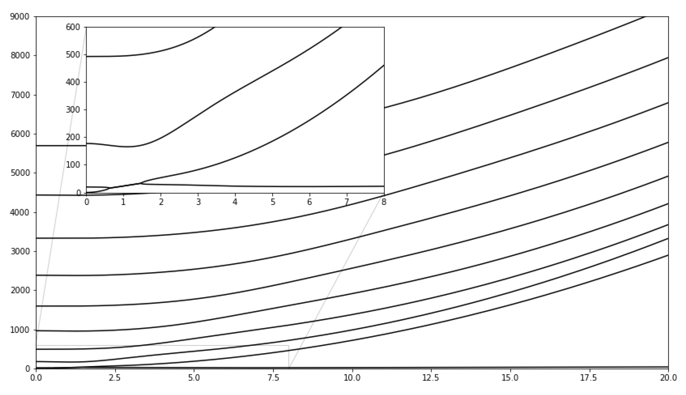
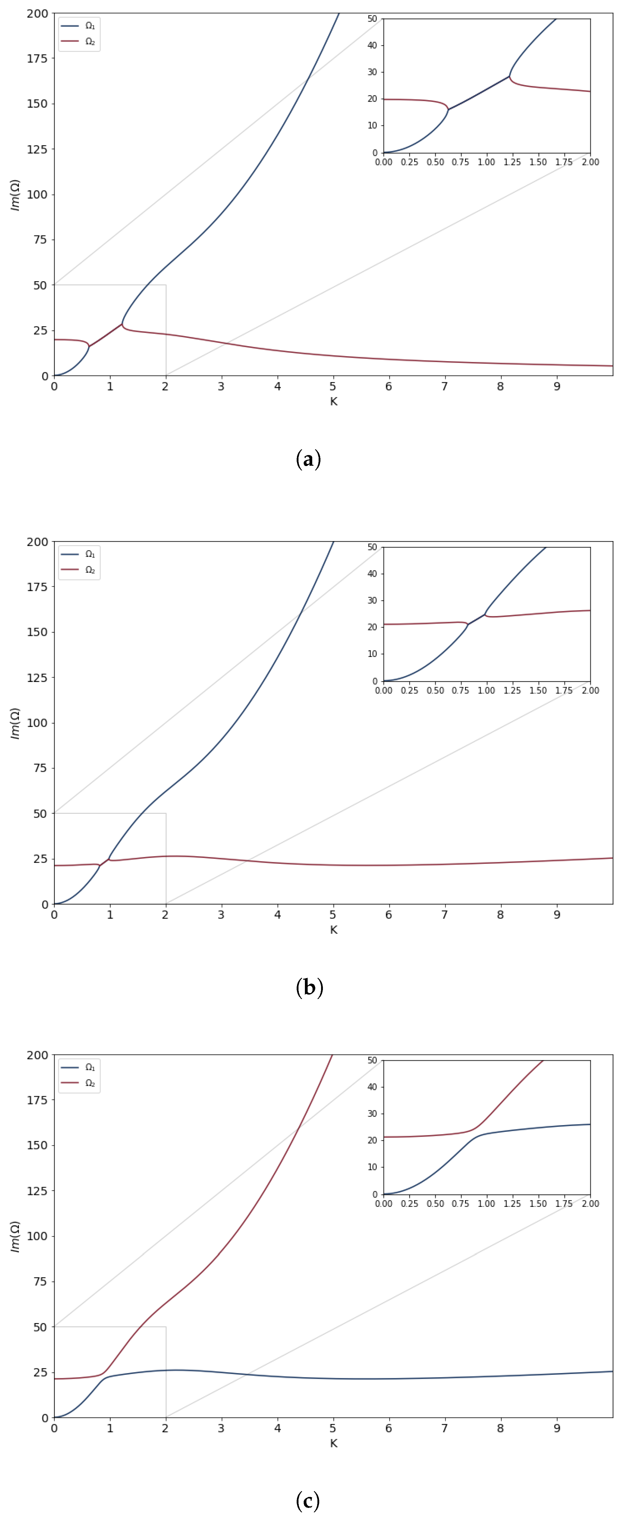
Having obtained Q for parameters p, s and K one may calculate mode frequencies. We present such results for a given material—glycerine—at some selected p values and as a function of scaled wave number K. The grand picture is this: at any given parameter settings one obtains infinitely many solutions, organized into branches as K changes (cf. Figure 1). In the following, the mode frequencies belonging to branch n will be denoted by . They emanate from values (46) or from zero. Most of them remain purely imaginary, but the lowest two may collide when increasing K. At such a collision, a bifurcation takes place, as in Figure 1 and Figure 2a, and two imaginary solutions Q may combine to complex solutions with non-zero real parts. Note that this bifurcation is also present in the parameters of Figure 3, but cannot be seen at the given resolution (it happens at very small wave numbers). The presence of complex Q solutions manifests itself in the appearance of a real part for the frequency. This means that wave propagation becomes possible. In that case the imaginary parts are the same, and the real parts differ in their signs only. As the value of p is increased, after a while such a collision no longer occurs, as in Figure 2c. This means that no wave propagation is possible because all modes are over-damped. The intermediate situation is approximately shown in Figure 2b. The mechanism of this possible bifurcation will be studied in more details in the next section (cf. Figure 4 and Figure 5). A bifurcation that is closely related to the one we find here at short wavelengths has already been found by Refs. [21,37]. In those works an infinitely deep fluid was studied.
In contrast, the bifurcation at long wavelength has been found explicitly here, and can be seen in Figure 1 and Figure 2a, where imaginary parts of the two lowest branches collide at a small wave number or long wavelength (we consider the wave number to be the control parameter when we speak about bifurcations). Below that wave number, all frequencies are purely imaginary, while above that wave number a real part arises (not shown in the figures), hence wave propagation becomes possible, as mentioned above. This bifurcation is also shown in Figure 6 on the parameter plane. There, wave propagation is possible in region IV, and a bifurcation at low wave numbers takes place when for a sufficiently low parameter p the red line between region I and region IV is crossed. For small wave numbers this line is parabolic, as quantified by Equation (75). This equation readily implies that the critical wavelength is , hence this bifurcation appears only in fluids of finite depth. The physical reason why this bifurcation happens can be understood from a simple order of magnitude estimate as follows. Let us consider a finite volume of the fluid, vertically from top to bottom, horizontally from a trough to the nearest crest. The main restoring force is gravity. If is the surface elevation, the pressure difference between the two vertical sides of the fluid volume is , and the restoring force (per unit perpendicular horizontal distance) is . Friction with the bottom is per unit surface (the characteristic vertical length scale is h, cf. Equation (74)), or for the whole segment (numerical factors are neglected), where is the wavelength. The mass of the fluid segment is . Hence, Newton’s second law reads in this case as
Further, we have the kinematic condition at the surface, , and the condition of incompressibility, . The partial derivatives may be estimated as and . By inserting these relations into Equation (48), we have
It is clear that for long waves friction prevails and the wave becomes over-damped. Indeed, the Ansatz leads to
This shows that for very long waves frequencies are purely imaginary. When wavelength is decreased, at around
a non-zero real part of the frequencies emerges. Note that Equation (51), obtained from rough order of magnitude estimates for the bifurcation point, agrees well with Equation (75).
There are a number of works where the bifurcation phenomena in surface waves were studied [23,43,44,45,46,47]. All these works considered the infinite depth fluid case. They fall into three categories: (1) a non-viscous case where bifurcation is due to nonlinearity [45,46]. (2) The presence of a surfactant where an interplay between dilational and capillary waves takes place [21,23,47]. (3) The presence of elastic membrane at the surface of the ideal fluid [43,44].
A further work, not belonging to the above categories, contains an ingenious application of bifurcation theory in order to prove the existence of linear waves and find the dispersion relation [48]. The system considered is a finite depth ideal (non-viscous) fluid without surface tension. Laminar rotational flow is assumed with constant vorticity (i.e., horizontal velocity is changing linearly with depth), and linear surface gravity waves at a fixed wavelength are considered. Stationary solutions are sought for in a coordinate system moving horizontally with constant speed compared to the fluid. This speed is considered to be the control parameter (in fact, the equivalent mass flux is used). Now, if the speed of the coordinate system is not equal to the phase speed of the waves, only the trivial, zero amplitude stationary solution exists, since the linear wave is a travelling wave as seen from that coordinate system. If, however, the speed of the coordinate system is equal to the phase speed, a further, nontrivial stationary solution emerges, whose existence is proved with mathematical exactitude under quite general circumstances. This technique has also been applied to study linear capillary waves in the same system, by neglecting gravity [49].
3. Parameter Dependence
3.1. Wave Modes
Plotting the real and imaginary parts of Equation (20) on the complex Q plane one usually observes several intersections, i.e., roots. They can be real, purely imaginary, or complex with non-zero real and imaginary parts (henceforth we shall use the term “complex” as an equivalent with “complex with non-zero real part and non-zero imaginary part”). In the first two cases the angular frequency (25) is purely imaginary, so these modes decay exponentially with time. Propagating modes are only possible if Q is complex.
3.1.1. Modes with Real Q
In this case, Equation (25) implies that , since the decay rate cannot be negative. We have found numerically that at a given parameter settings (s, p, and K) there can exist zero, one, or two real modes (due to the symmetry of the solutions, we consider roots only in the first quadrant). There is always a trivial solution . Then, we get from Equation (12), so this solution is irrelevant.
In case of nontrivial real solutions, the decay rate is always smaller than . Velocity components may be calculated from Equations (3), (4), (12) and (26). Provided that coefficient A is real, u is real, too, while w is purely imaginary, so there is a 90° phase shift in their x-dependent oscillations.
3.1.2. Modes with Imaginary Q
In this case the decay rate is always larger than . Such modes exist at any parameter setting, moreover, there are infinitely many of them. Indeed, if Q is purely imaginary as and its modulus is large, Equation (20) reduces to
or, substituting ,
Now, if (n being an integer), the left hand side is positive, and if , the left hand side is negative. Therefore, between these values there is a root for any (arbitrarily large) n. The distance between imaginary roots is approximately constant and independent of viscosity.
As before, the phase of velocity components does not change with depth, while there is a 90° phase shift between the x and z components. It is interesting that imaginary Q causes an oscillatory behaviour with depth.
3.1.3. Modes with Complex Q
On the basis of our numerical investigations, we believe that at a given parameter setting at most one such mode can exist. If there exists one, then at the same parameter setting no mode with real Q can exist. This time the phases of velocity components do change with depth. An oscillatory dependence on depth is in principle present, but much less pronounced than in the imaginary case.
3.2. Bifurcations
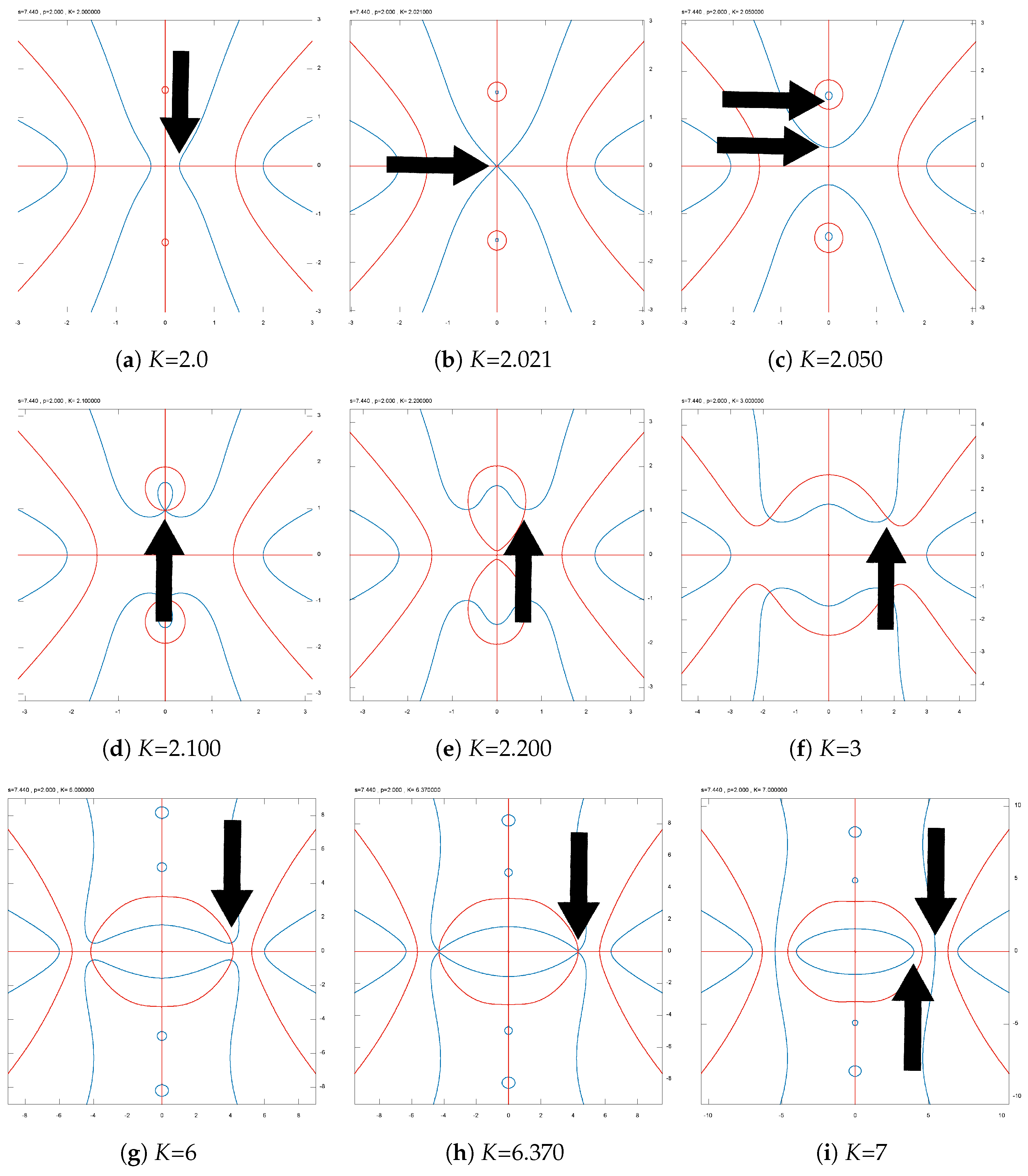
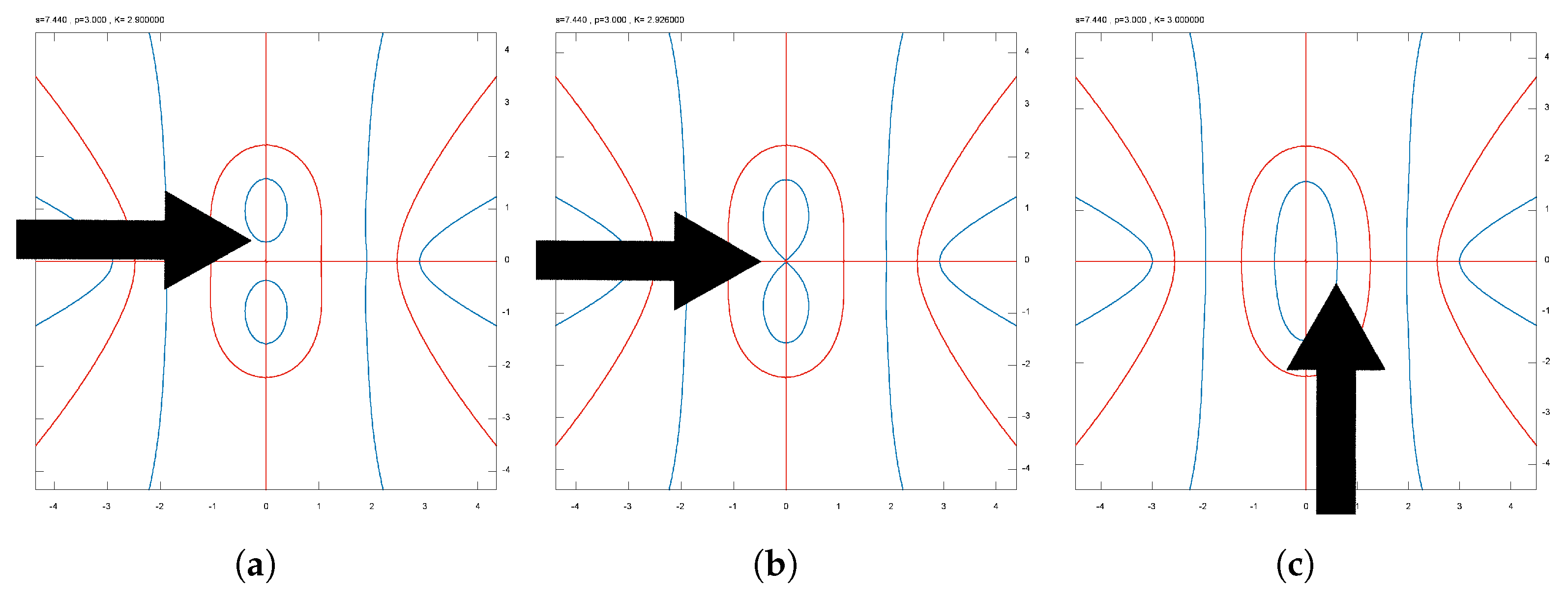
If, at the given s and p parameters one adjusts K, the type and number of solutions changes. This is shown in Figure 4a–i where and . The left hand side of Equation (20) divided by is plotted (this factor is chosen to avoid exponential growth.) on the complex Q plane, the zero level lines of the real part in blue, and those of the imaginary part in red. Hence, intersections of red and blue curves are solutions of Equation (20). As wave number K grows, these solutions are moving on that plain and display bifurcations. Since there are other (sometimes non-physical) solutions present, we denoted by black arrows the solutions we wish to focus on. In Figure 4a one can see a real solution. A bifurcation is shown in Figure 4b, where the real solution and its mirror image collide at the origin, and a further increase of the wave number gives rise to an imaginary solution (cf. Figure 4c, lower arrow) and its mirror image.
Increasing the scaled wave number K further, one can observe that that two imaginary solutions in Figure 4c collide (see Figure 4d) and give rise to a complex solution (see Figure 4e). This complex solution gradually goes down to the real axis (cf. Figure 4e–h) and decays to two real solutions (Figure 4i) which survive any further increase of K.
Choosing the parameter values and , one has a different scenario, see Figure 5a–c. This time only a single bifurcation takes place, namely, an imaginary solution and its mirror image collide at the origin (see Figure 5b) and give rise to a (second) real solution (cf. Figure 5c).
These observations allow us to find the mathematical conditions of the bifurcations, which mean transitions among different types of possible modes. These conditions appear as curves on the K-p plane and partition that plane according to the types of possible solutions. Since the p-dependence is simpler than the K-dependence, we find these curves at constant K by varying p, rather than varying K at constant p, as has been done above when demonstrating the bifurcations. The curves are certainly the same.
![Fluids 08 00173 g004]()
![Fluids 08 00173 g005]()
Figure 4.
Zero level lines of the real (blue) and imaginary (red) part of Equation (20) divided by plotted on the complex Q plane at parameter values and .
Figure 4.
Zero level lines of the real (blue) and imaginary (red) part of Equation (20) divided by plotted on the complex Q plane at parameter values and .

Figure 5.
Zero level lines of the real (blue) and imaginary (red) part of Equation (20) divided by plotted on the complex Q plane at parameter values and . (a) . (b) . (c) .
Figure 5.
Zero level lines of the real (blue) and imaginary (red) part of Equation (20) divided by plotted on the complex Q plane at parameter values and . (a) . (b) . (c) .

In all the above numerically discussed cases (Figure 4 and Figure 5) at the birth of new solutions one can observe that by approaching the critical parameter the zero level lines of the real part of Equation (20) develop an edge, and at bifurcation they become (locally) two straight lines crossing each other on the real and/or the imaginary axis (Figure 4b,d,h and Figure 5b). This means that at the bifurcation point the derivative of the line is undetermined, i.e., it has a form . Note in passing that it is equivalent with the condition that the second derivative becomes infinite. Let us denote for brevity the real part of Q with and its imaginary part with (i.e., ), further, the left hand side of Equation (20), divided by be . Then the zero level line of the real part of D is given by
Here ℜ stands for the real part. Taking its derivative with respect to , we get
hence the derivative of the curve is written as
Here ℑ stands for the imaginary part (without i). It follows that at bifurcation
must be satisfied, together with . Now it is easily seen that is real along both the real and the imaginary axis, while is real along the real axis and imaginary along the imaginary axis. Therefore, in case of a bifurcation on the real axis we have
i.e., two real equations for the two real parameters and p (at constant K and ). Similarly, in case of a bifurcation on the imaginary axis we have
again two real equations for the two real parameters and p.
In terms of these functions we have (cf. Equations (58) and (59))
and (cf. Equations (60) and (61))
for bifurcations on the real and imaginary axis, respectively. In these cases, Equation (65) or Equation (67) is solved numerically to get or , respectively, then the solution is inserted into Equations (66) and (68), respectively, which in turn are solved for p at constant K and , taking into account Equation (35).
As for the transformation of an imaginary solution to a real one at the origin, mentioned above, for the critical line one obtains
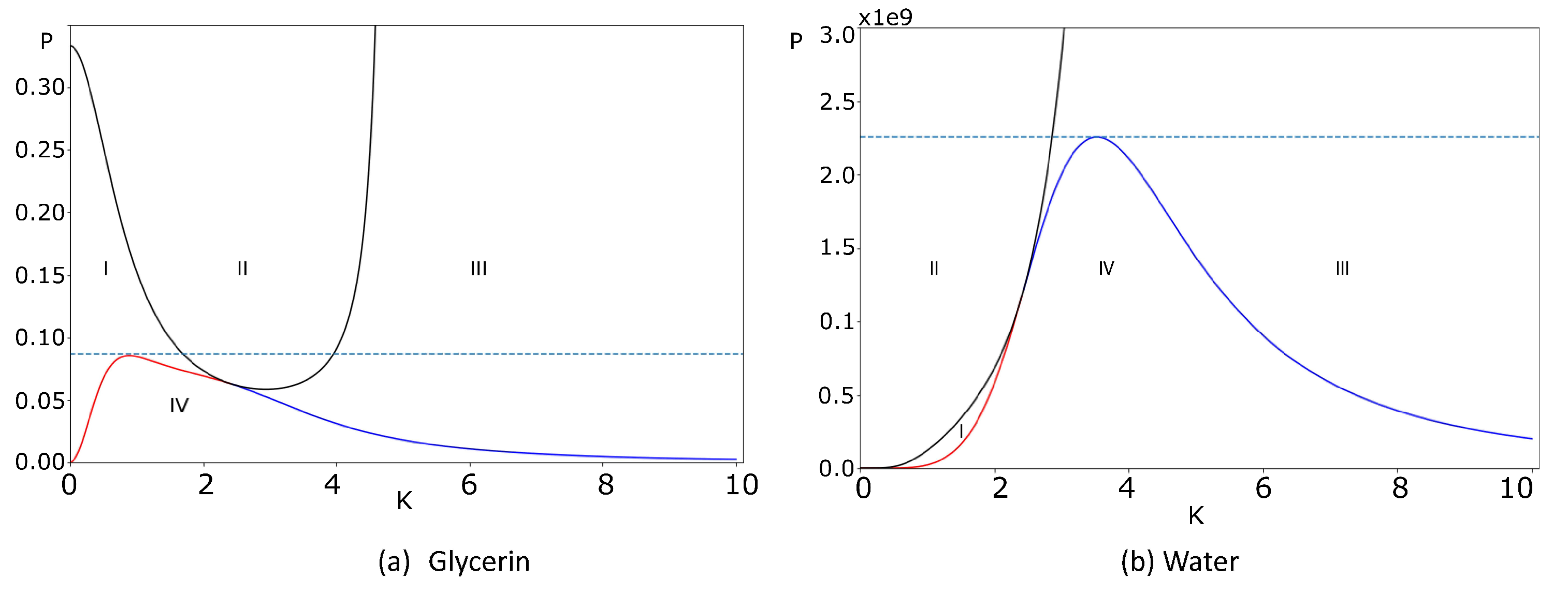
Since both and are even functions of Q, it follows that , hence Equations (65) and (67) are automatically satisfied for and , respectively. The results are plotted in Figure 6a,b for glycerin and water, respectively. These two figures are very much different, not only in the shape of the curves, but in their vertical scales, in the first place. The values in Figure 6b are of order . Such a huge difference needs an explanation. When we solve the Equations (66), (68), or (69) for p, we actually solve an equation
where a is a function of K alone and is of order . The solution of Equation (70) is
where stands for the inverse of function . It is easily seen that
and
Therefore, when , the solution is approximately , as is the case for glycerin. In contrast, if , then the solution is . This happens in the case of water and mercury, and we get huge values for p, except for very small K values. These large p values are equivalent with extremely small layer widths (cf. Section 4). In fact, they are so small that the bifurcations in question are hardly observable in case of water or mercury as well as other fluids with low viscosity. They might be observable, however, in more viscous fluids such as glycerin.
In short, the physical reason of the difference between Figure 6a,b is that in case of water the viscosity is much smaller than in the case of glycerin (the surface tensions in the two cases are comparable) and this is reflected in the corresponding values ( for water and for glycerin ). The two order of magnitude difference in the values of for water and glycerin is further magnified by the cubic functional dependence (73).
On the other hand, for small enough K values, condition is satisfied, hence in that limiting case the parameter space regions become independent of . This is natural, since in the long wavelength limit the impact of the surface tension vanishes.
In Figure 6 the red line means the onset of the creation of a complex solution at the imaginary line, i.e., the solution of Equations (67) and (68). The bue line is the same at the real line (cf. Equations (65) and (66)), while the black line is the onset of the crossover from the imaginary to the real solution at the origin (Equation (69)). It is obvious that these lines must have a common point. The lines partition the parameter space to four regions, denoted in the figures by Roman numbers:
- I.
- Only imaginary solutions (infinitely many of them) are present;
- II.
- There is a single real solution and there are infinitely many imaginary solutions;
- III.
- There are two real solutions and there are infinitely many imaginary solutions;
- IV.
- There is a single complex solution and there are infinitely many imaginary solutions.
Figure 6.
The maximal parameters p versus the scaled wave-number K for glycerin (a) and water (b). Note the vertical scale in (b). The red line signifies the emergence of complex solutions at the imaginary line, while the blue line represents the real solutions obtained from Equations (65) and (66). The black line denotes the onset of the crossover from imaginary to real solutions at the origin.

Asymptotics and some special cases of the bifurcation curves are the following.
- 1.
- Imaginary to complex Q (border between regions I and IV, the red curve in Figure 6):For small K () we have
- 2.
- Complex to real Q (border between regions IV and III, the blue curve in Figure 6):For large K we haveThis implies (cf. Equations (21)–(24) and Equations (30) and (31)) that the transition to the over-damped mode happens at wavelengthIt is remarkable that this value does not depend on layer thickness h or gravity of Earth g, as it is a purely material constant. Numerically, we get for water, for glycerin and for mercury. In our opinion, this effect cannot be observed in water or mercury, but might be observed in glycerin. It is questionable if hydrodynamics are applicable at the scales obtained for water and mercury, albeit at least one study states that it is applicable down to the nanoscales [28]. It is obvious that in case of these short waves gravity does not play a role. Here we demonstrate, that our more general setup leads to the right results in this limiting case. There are other situations, however, when gravity becomes important. This happens, e.g., at the bifurcation at long wavelengths. Gravity and surface tension become equally important when the two bifurcations (at large and small wavelength) are close to each other, as in Figure 2a.
- 3.
- Imaginary to real Q (borders between regions I, II, and III, the black curve in Figure 6):For small K we haveAt parameter p diverges asFor a given material this implies (cf. Equation (35))
- 4.
- The common point of the bifurcation parameter curves (red, blue, and black lines in Figure 6 satisfiessince . This impliesThe solution of this equation yields for the coordinates of the common point
4. Minimal Layer Thickness Necessary for Wave Propagation
Viscosity not only damps waves, but it can even prevent their propagation. Indeed, propagation, mathematically, a real part of the complex angular frequency, appears only in region IV (cf. Figure 6). This implies that no gravity-capillary waves can propagate if p is large enough (or, equivalently, if the layer width is small enough). Further, even if the layer thickness is larger than the critical value, neither very long, nor very short waves can propagate.
The critical layer thickness is found from the maximum point of the curves bordering region IV in Figure 6 (cf. Equations (65)–(68)). This depends on the material parameter , so we present the results in Table 1. Clearly, for water and mercury the critical layer width is so extremely small that at such scales even the applicability of standard hydrodynamics is more than questionable.
5. Particle Motion at Surface
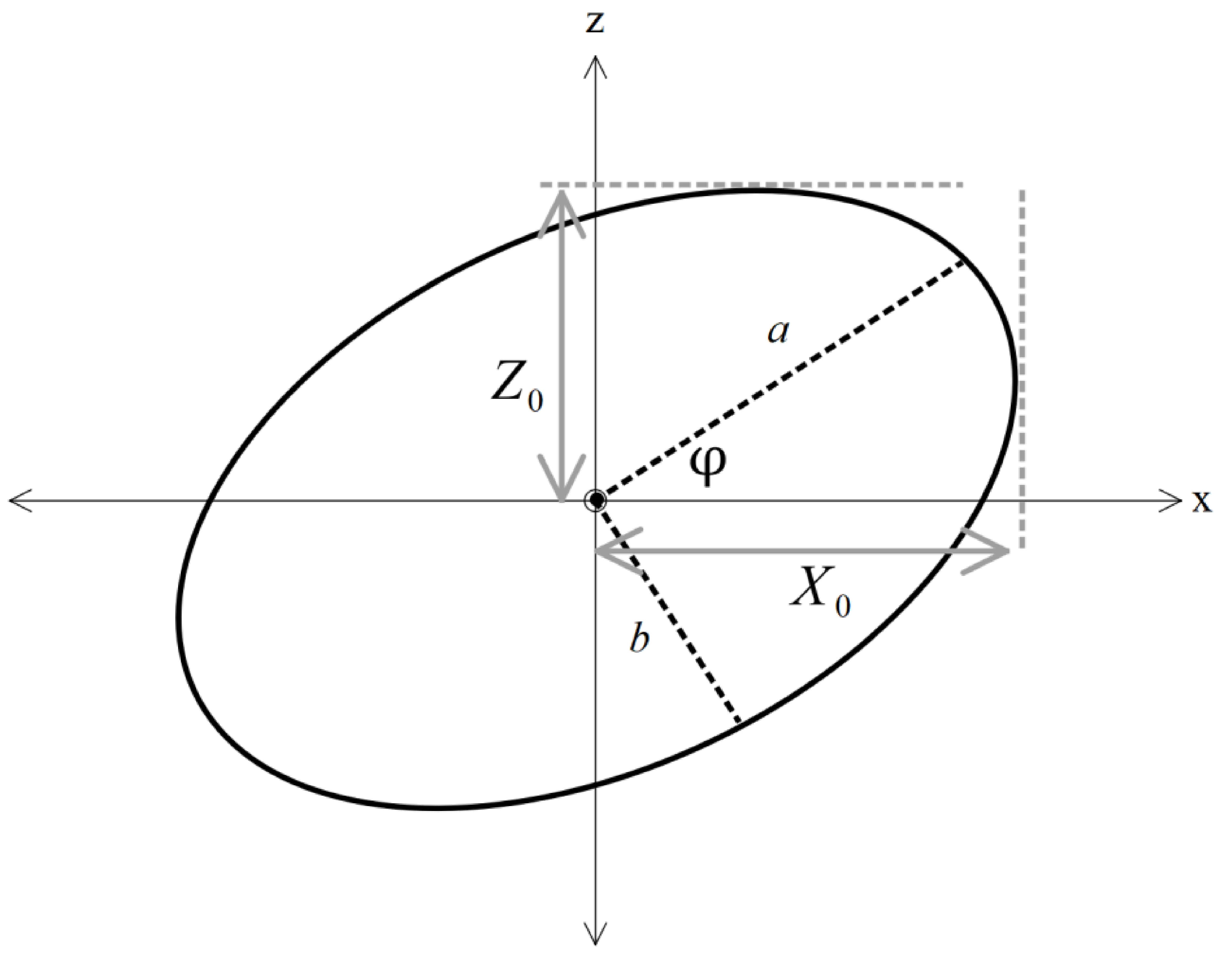
In this section, we focus on the numerical simulation of particle trajectories associated with wave patterns at the surface of the fluid. Since we are considering linear waves, both the horizontal and vertical motion is that of a damped harmonic oscillator. If we neglect damping, the resulting motion due to these two perpendicular harmonic oscillations results in a general elliptical motion. Note that in the presence of damping, the actual motion will be a spiral. The parameters of the ellipse (see Figure 7), main axis a, small axis b, and angle of the main axis made with x direction, are related to the horizontal and vertical amplitudes and phase difference. The relevant relations are the following:
Angle of main axis compared to horizontal, , is given by
Here
and
where and are phases of the horizontal and the vertical oscillations, respectively:
Explicitly,
and
According to Equations (93) and (94), when Q is a real, the value of is , but if Q is purely imaginary, then the value of is .
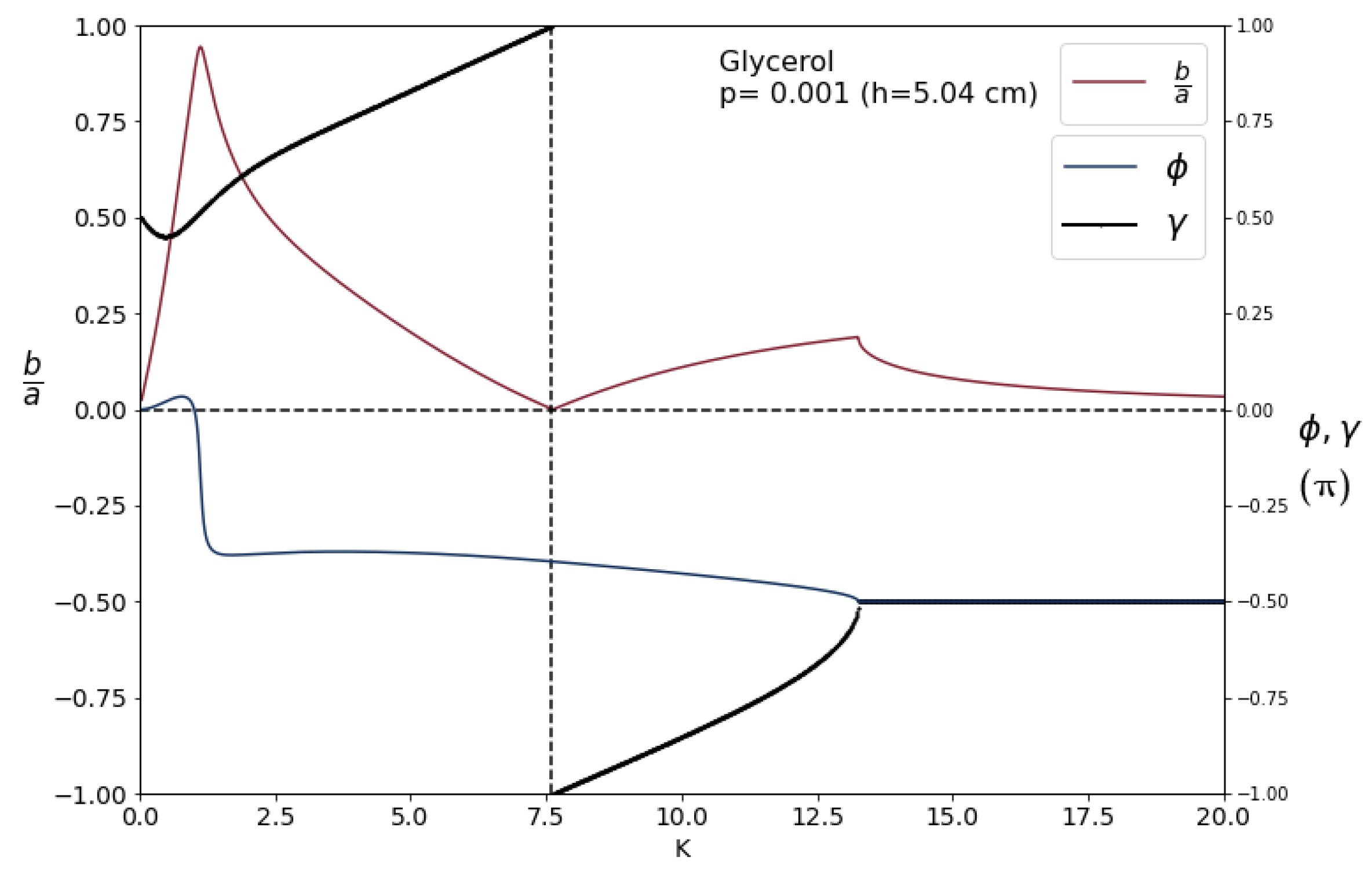
These parameters are plotted versus scaled wave number K in Figure 8 at . Wave propagation is permitted from to , as seen in Figure 3 (Except for very small K values where the motion always becomes damped. At the resolution of the figure, this regime can not be seen). The motion is virtually linear () for small values of K but quickly transforms into a circle with close to unity at . The angle that the main axis makes with the horizontal, , is almost zero up to this point, then it rapidly takes 90 degree turn and remains around that. The ellipse gets narrower for wave numbers greater than unity () and at wave number , it degenerates into a linear segment. The corresponding motion is nearly perpendicular to the surface. The ellipse then gets a little bit thicker. Both the horizontal and vertical motion are excessively over-dampened at . The change in the phase difference between horizontal and vertical motion is also displayed. It is clear that with K being approximately 1, the phase difference is approximately . When the ellipse degenerates into a line segment at , the phase difference reaches . At the bifurcation point, the phase difference hits .
6. Time Evolution of Surface Elevations
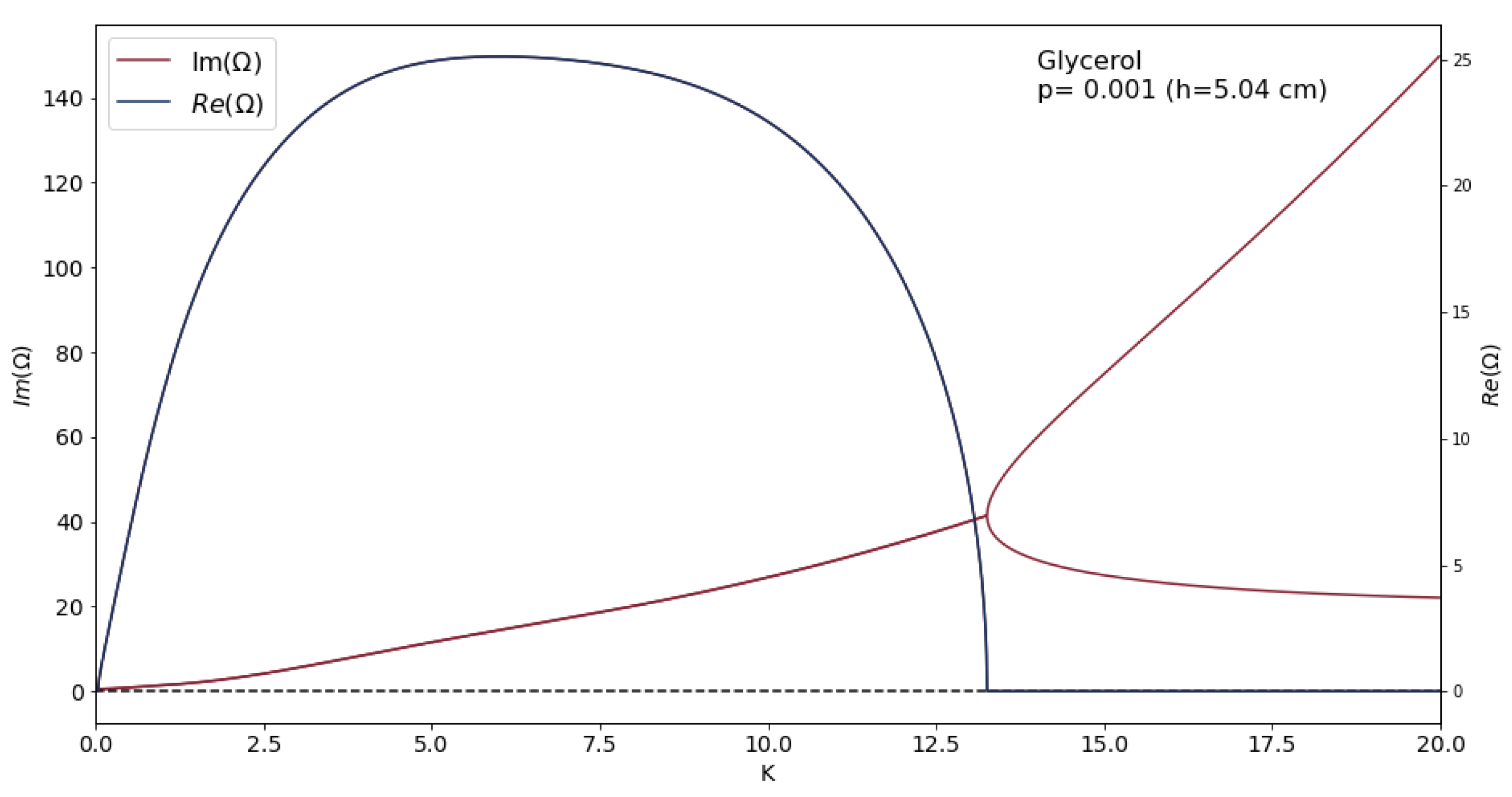
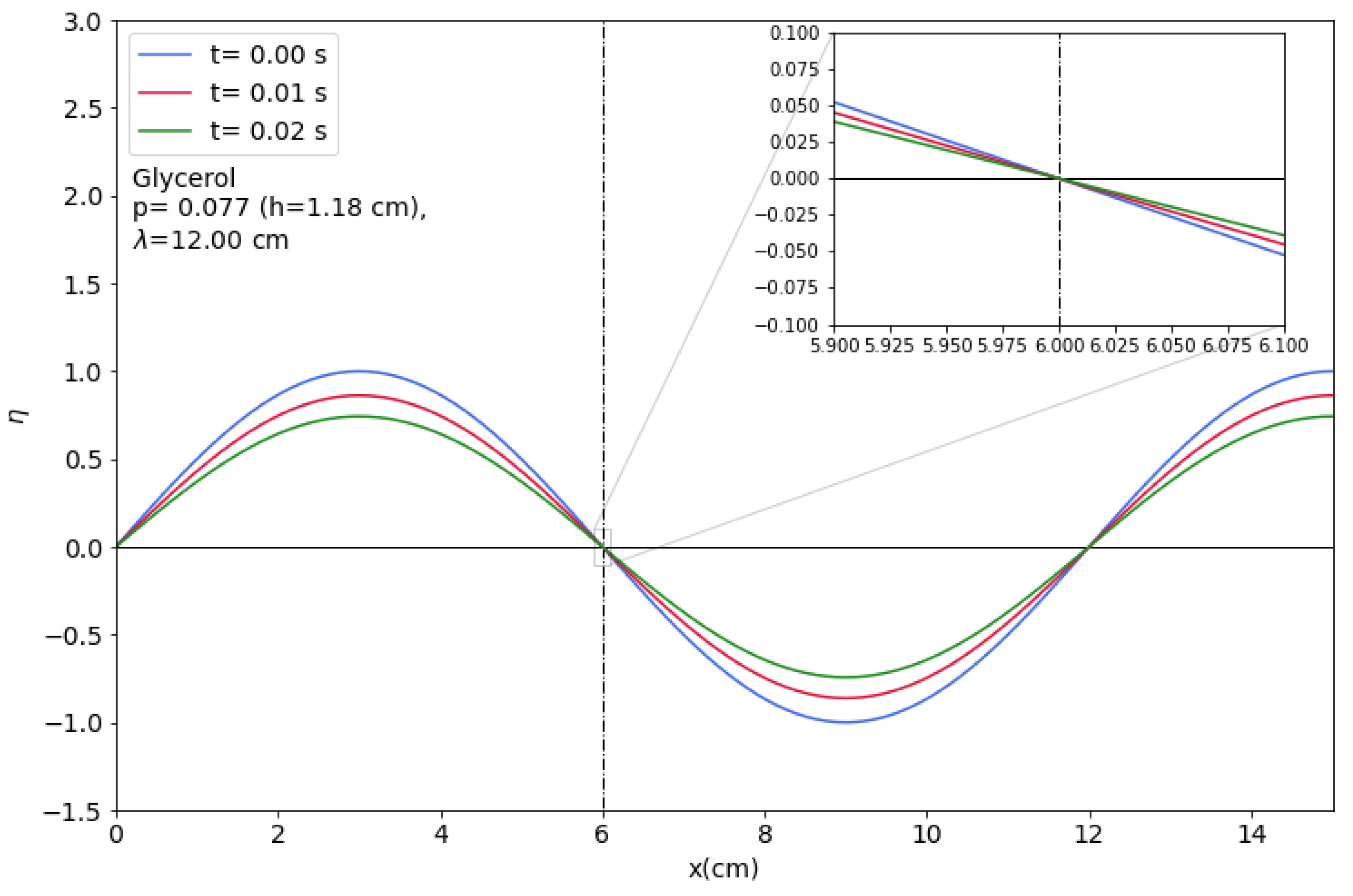
Figure 9, Figure 10, Figure 11, Figure 12, Figure 13, Figure 14 and Figure 15 demonstrate the time evolution of a propagating wave in a fluid, along with the associated dispersion relations. We have chosen glycerin as the fluid medium due to its physical properties, as other fluids may require a thinner layer for observation of the phenomena. Then, the critical thickness for glycerin is 1.1 cm, for water is m, and for mercury is m, which is the reason we have chosen the glycerin for simulation. We limit our study to the lowest two branches of the dispersion relation, because, as shown in Figure 1 these branches have the longest lifetime and, i.e., they are the least damped.
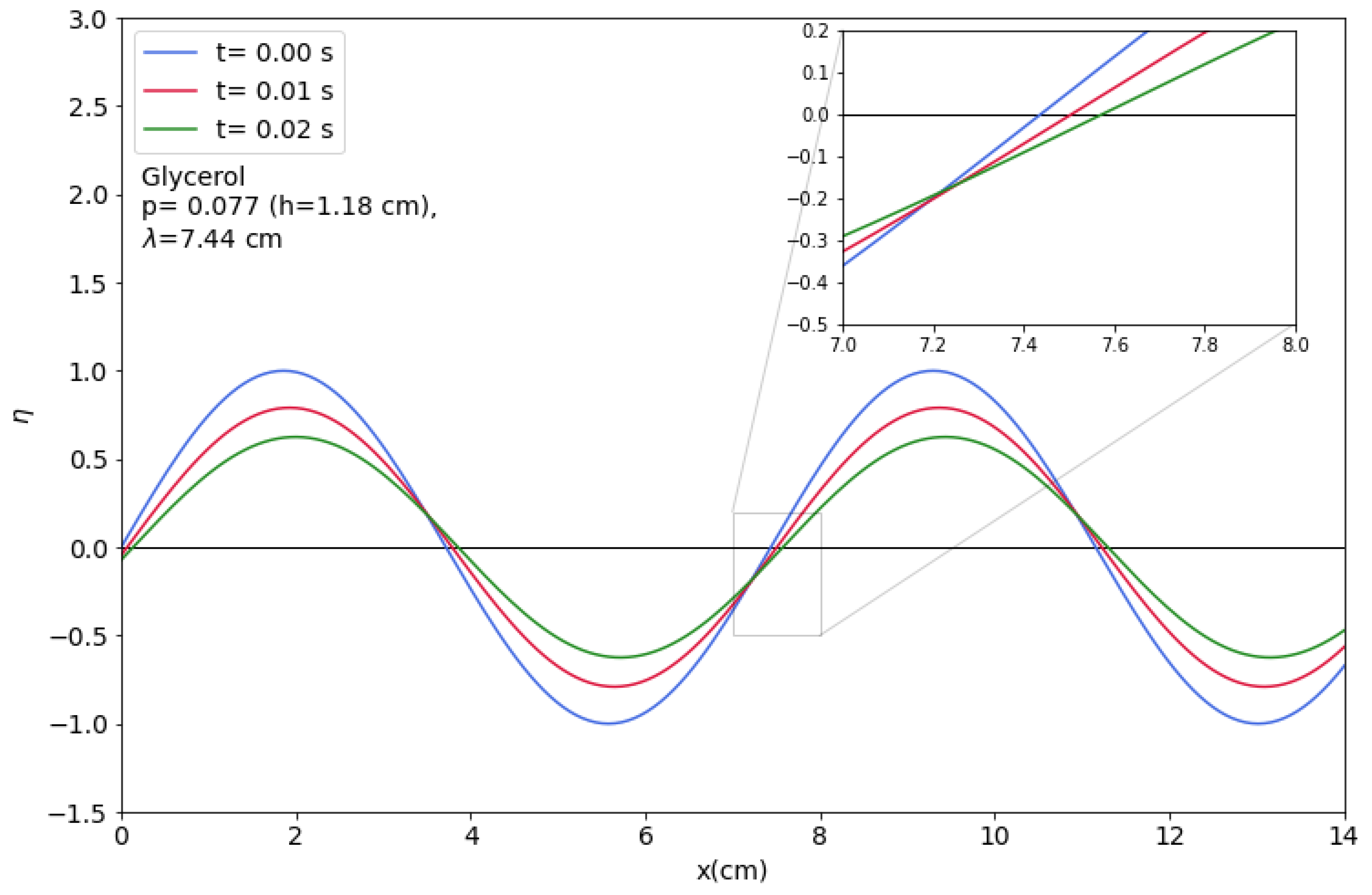
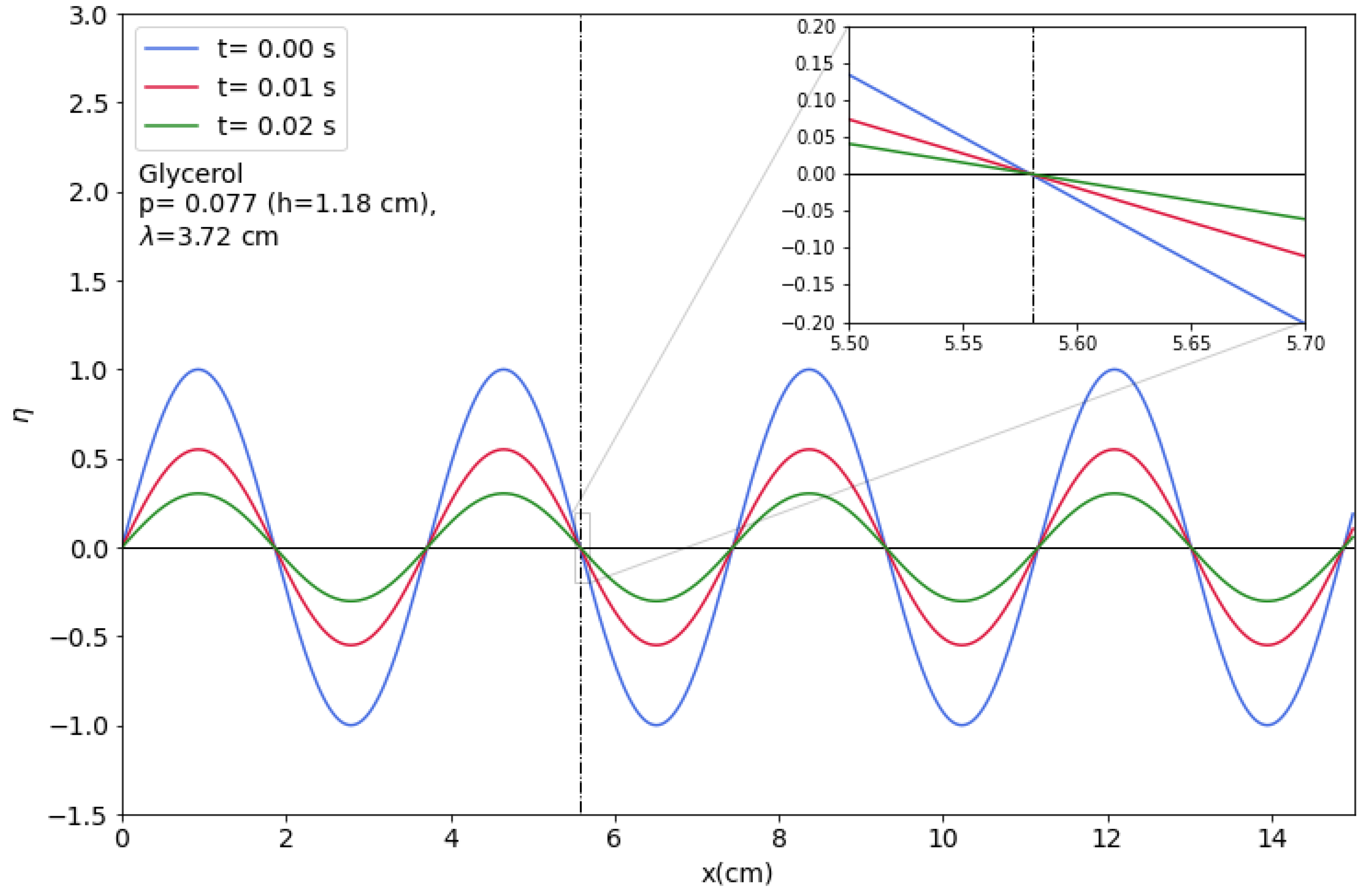
We aim to establish a correlation between theoretical predictions and empirical observations. The findings indicate that wave propagation is detected at a particular wave-number of , within a narrow range, when , which is in proximity to the critical value of . Conversely, no propagation is observed at longer wavelengths, such as , or at shorter wavelengths, such as , as illustrated in Figure 9, Figure 10 and Figure 11. Figure 9 depicts the over-damped mode characterized by a long wavelength. At a specific wavelength of , a wavenumber of , it can be observed that wave propagation is not feasible due to the nodes remaining in the unchanged position (cf. Figure 2a). It should be noted that surface tension plays a minor role in this context. The nodes in Figure 10 are observed to be in motion due to the occurrence of wave propagation at a wavenumber of . This is in agreement with Figure 2a. At , the wave in Figure 11 exhibits over-damping. Surface tension is a dominant phenomenon in this particular regime.
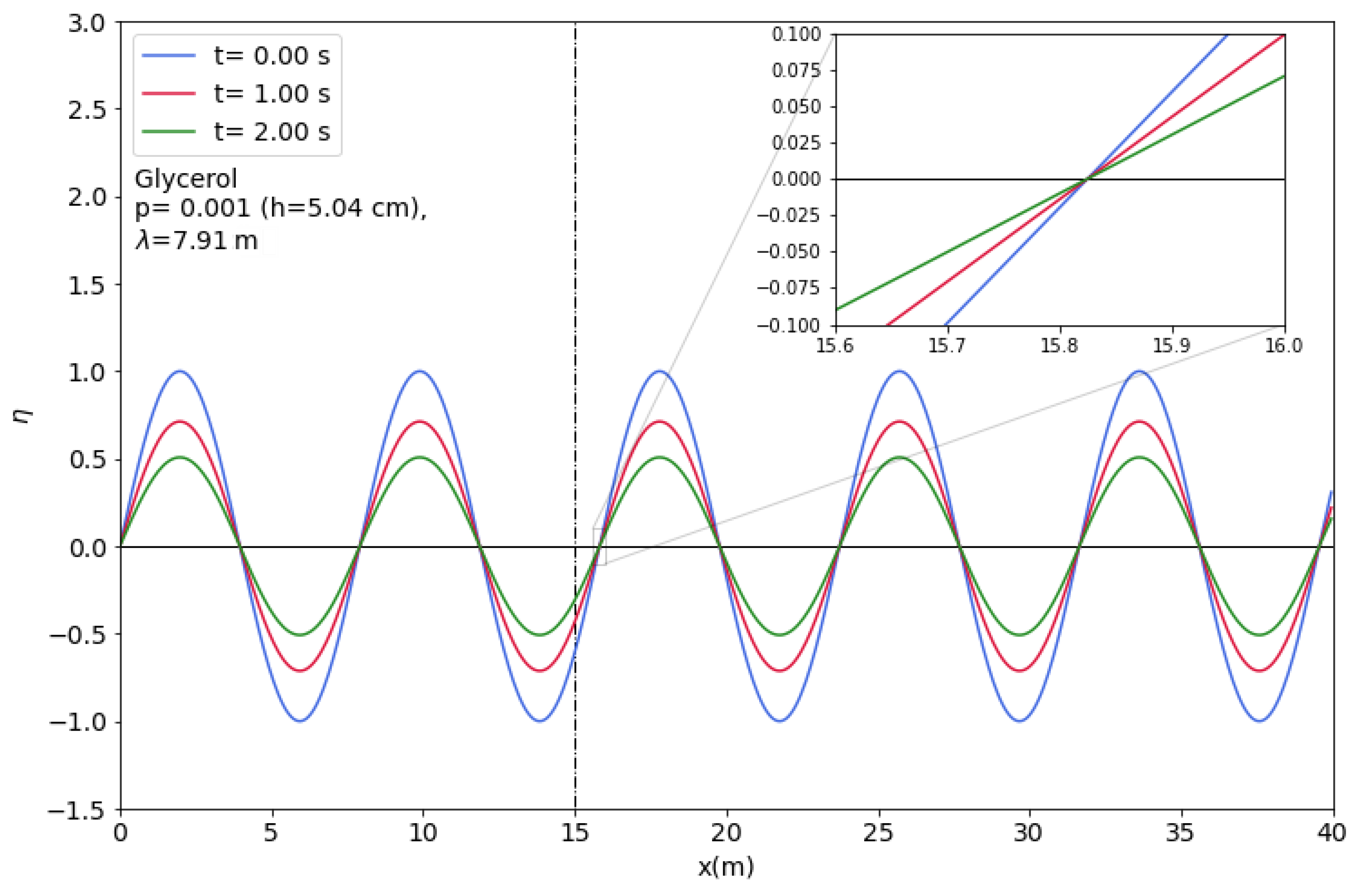
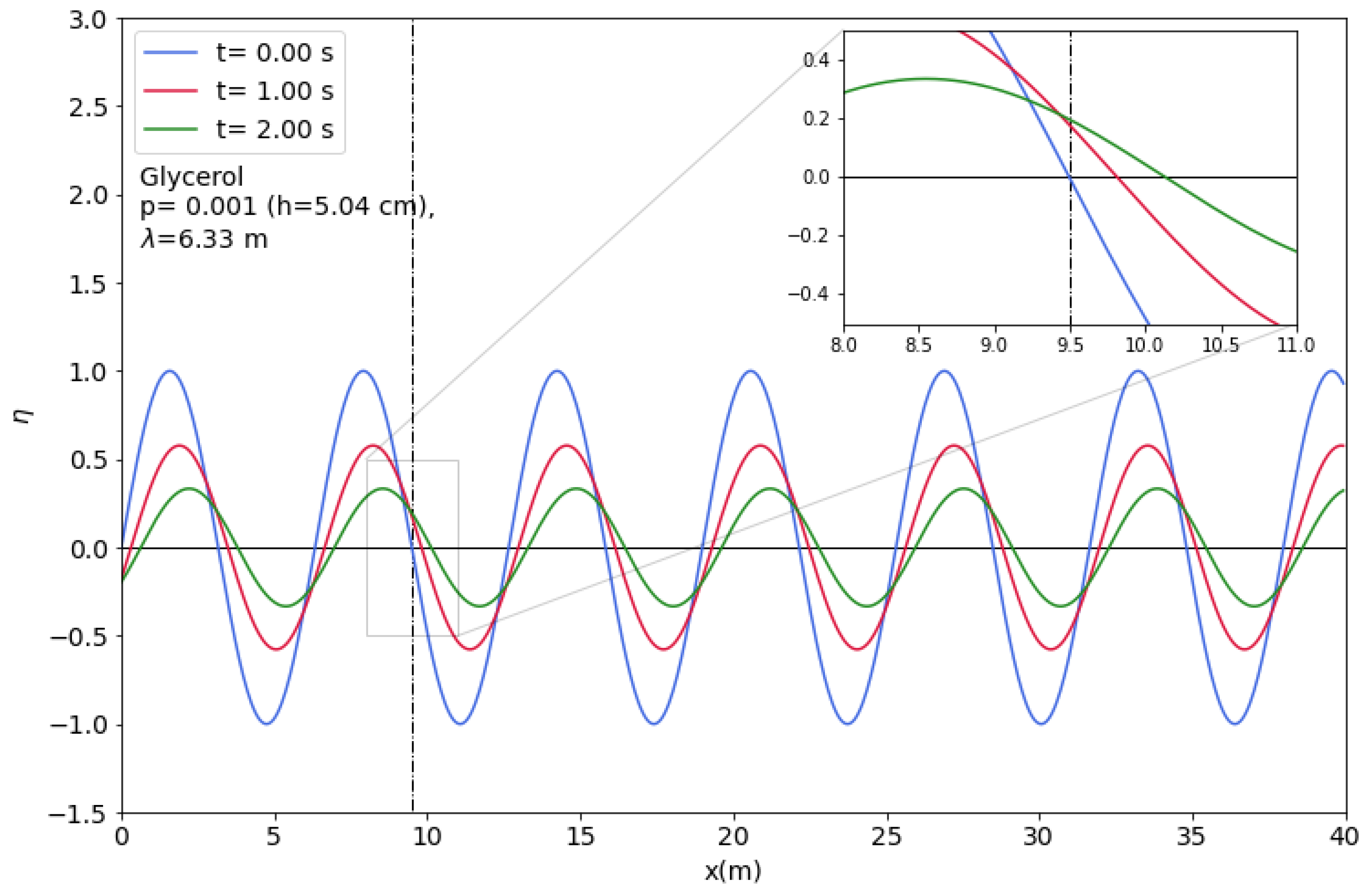
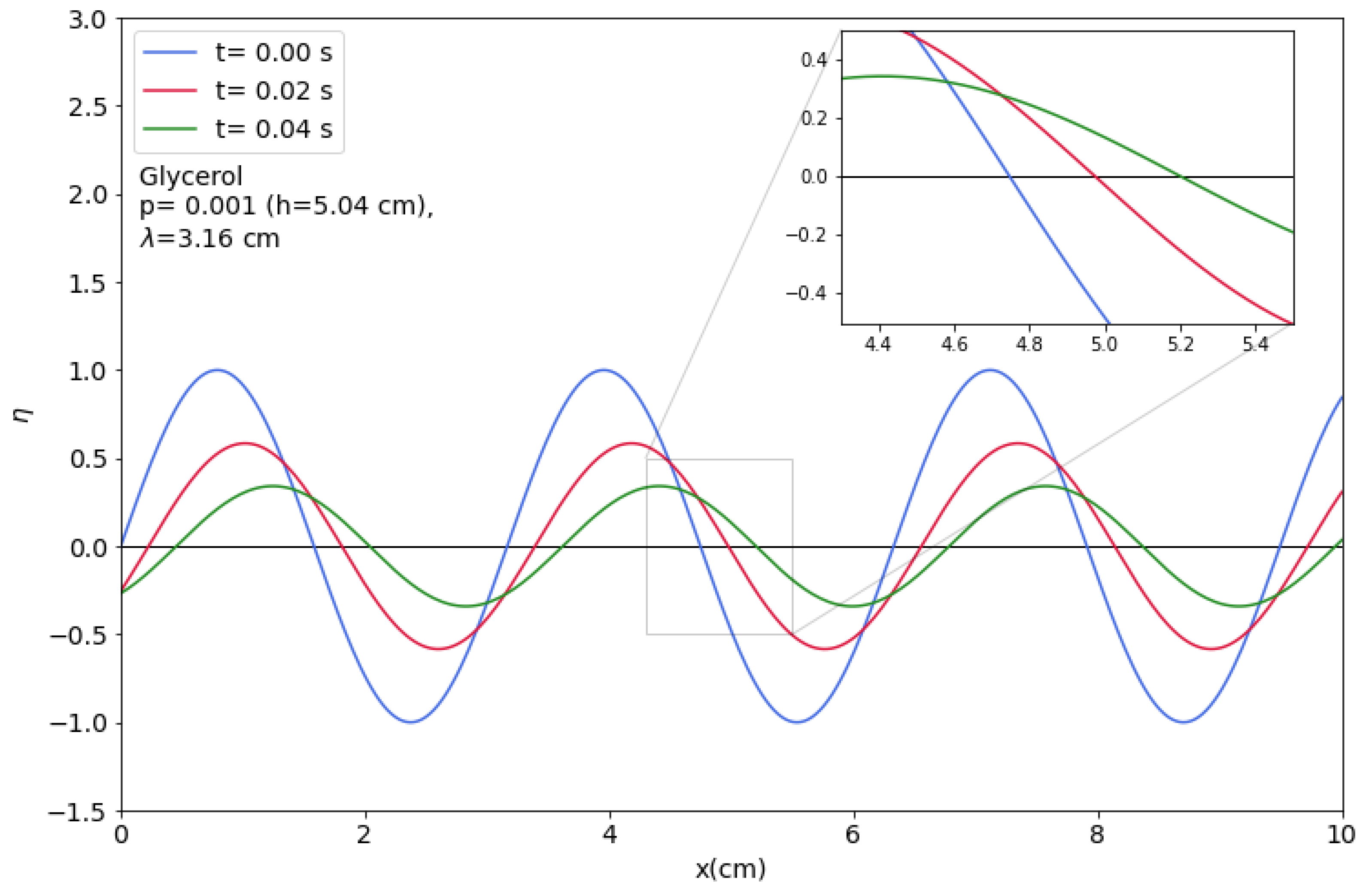
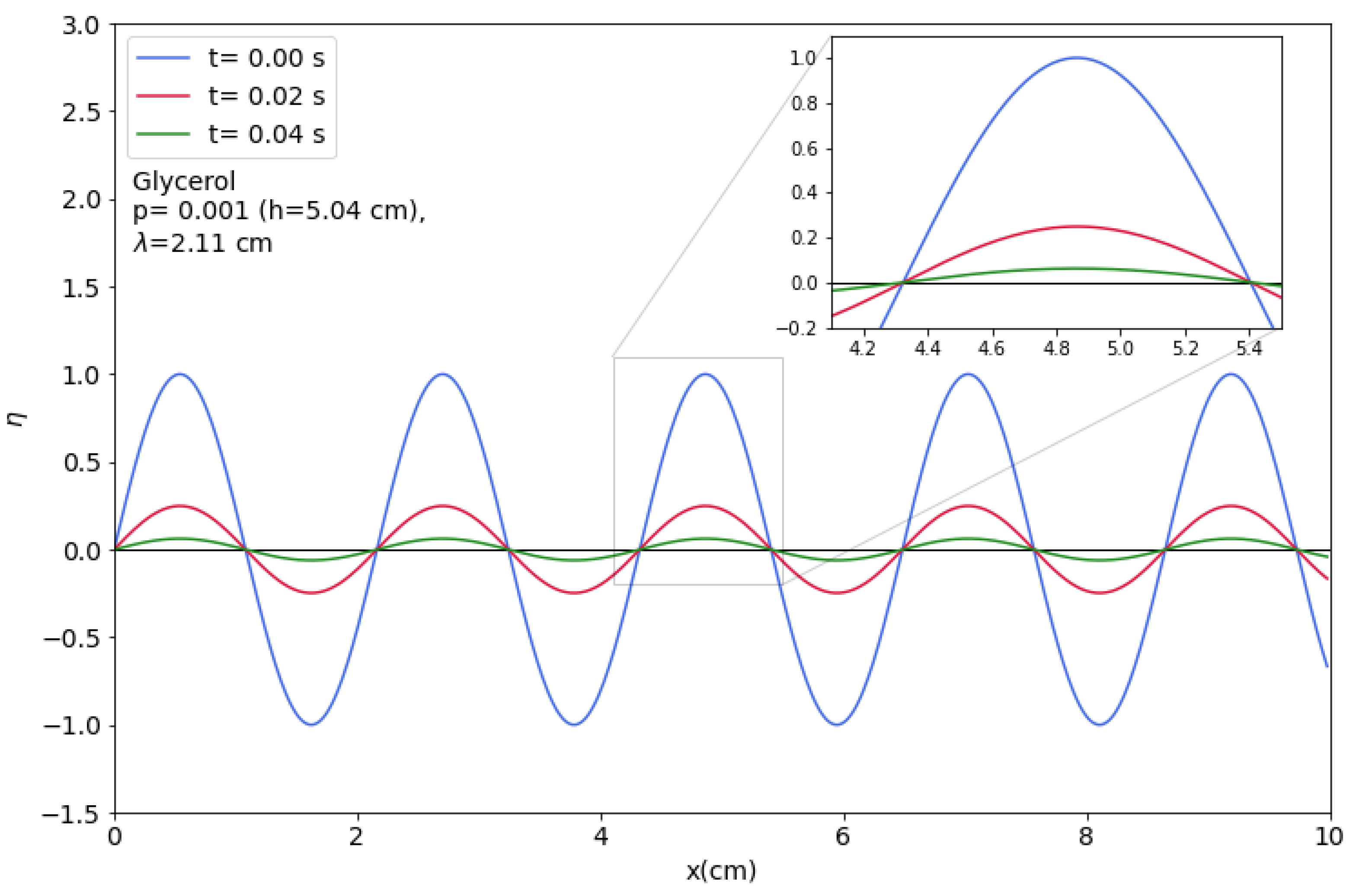
At , the range of wavelengths that undergo propagation is wider. However, it is worth noting that a non-propagating long-wave mode develops at a wavelength of 8 m in a fluid layer of 5 cm, which poses a challenge for observation (refer to Figure 12). Figure 13 illustrates the observation of a travelling wave with a shorter wavelength of . The demonstration shows the limited wavenumber spectrum within which long wavelength over-damped modes exist. Figure 14 shows the propagation of waves at the same layer width, with a wavelength of . It should be noted that the velocity is significantly greater, as evidenced by the time labels. The propagation of waves with a shorter wavelength, specifically those with a wavelength of , is prohibited, as shown in Figure 15.
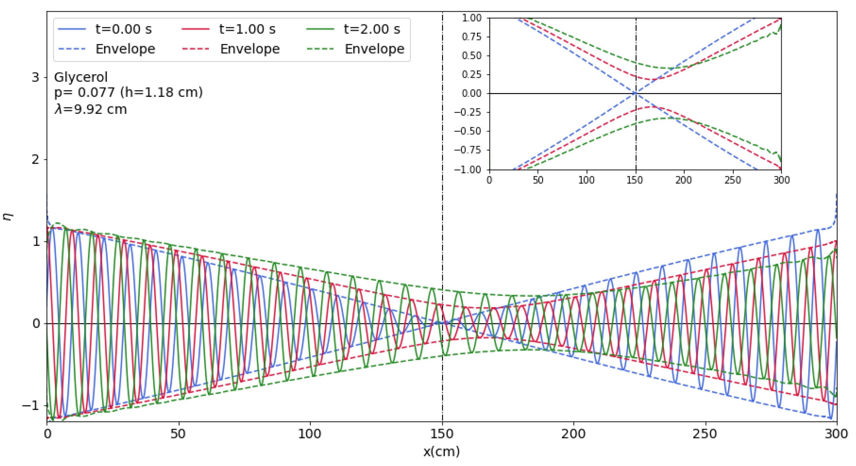
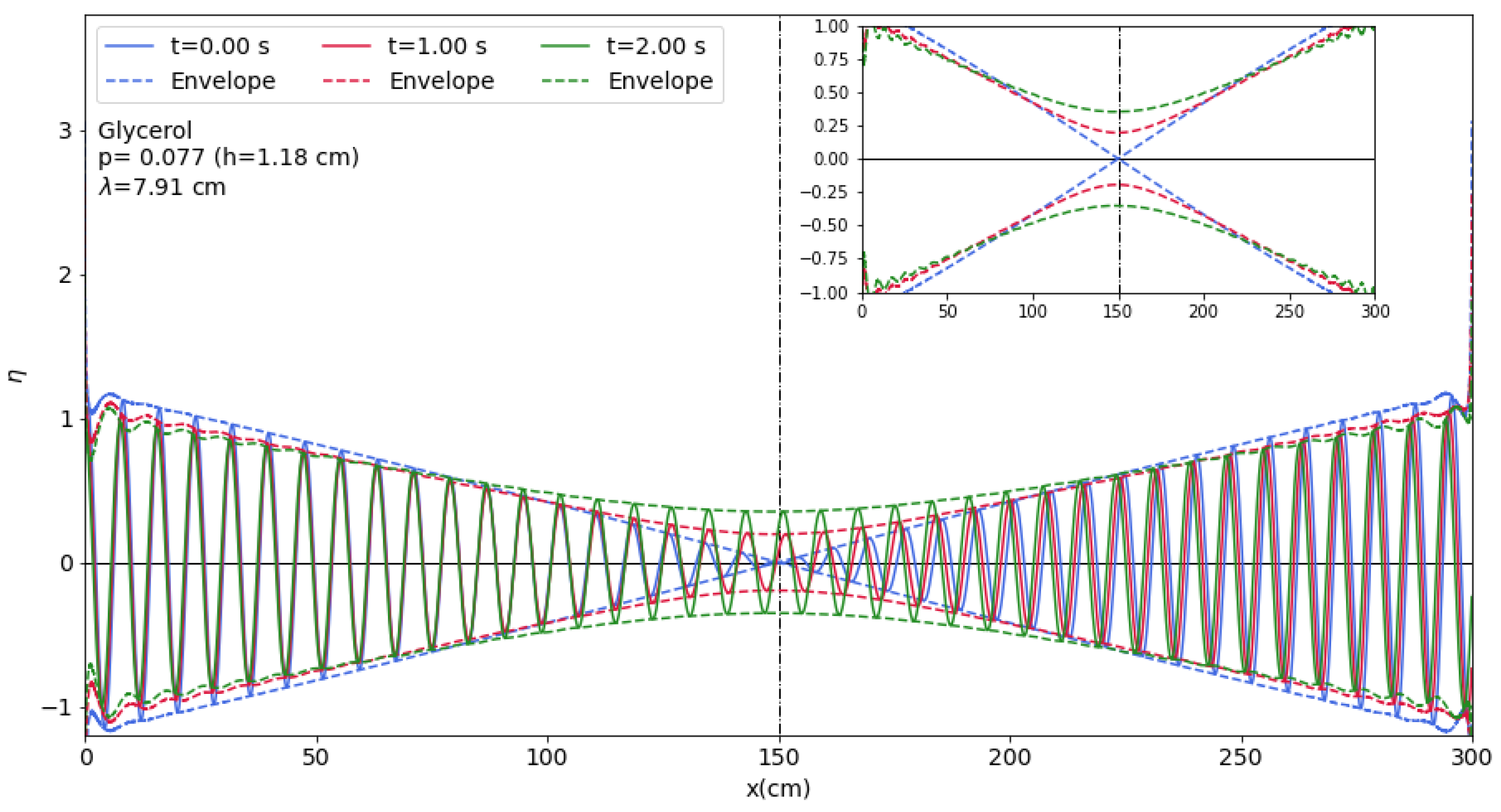
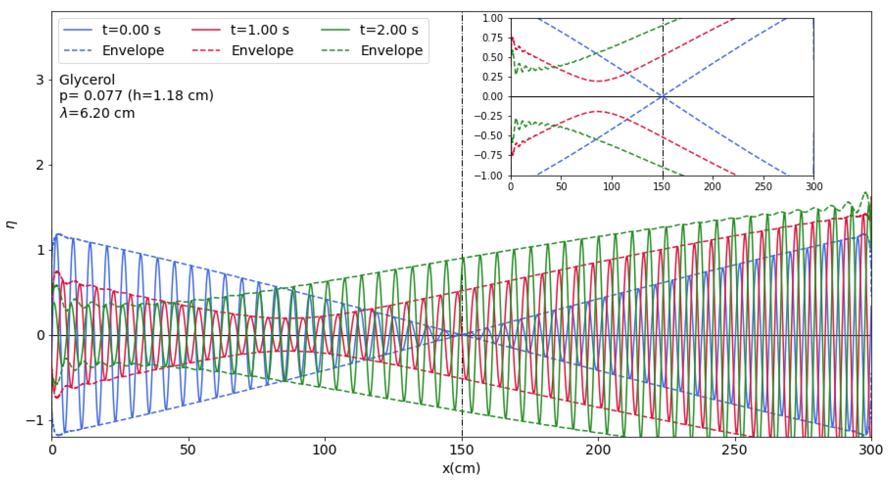
For the purpose of demonstrating the group velocities present in the propagating modes, we overlay two wavelengths that are in close proximity. Specifically, we consider the expression , where both waves are propagating towards the right. Nevertheless, the direct observation of this phenomenon appears improbable due to significant damping. In order to show the motion of the envelope, the superposition is amplified at a rate of , where denotes the lesser decay rate. Figure 16 illustrates the superposition of two waves with two nearby wavenumbers ( and ) at three consecutive time intervals. The direction of their travel is towards the right. At the onset, the envelope exhibits a node. At a subsequent time interval, the node expands to form a bottleneck. The position of the bottleneck is moving to the right, which indicates that the group velocity is also positive in this scenario. The phenomenon of broadening can be attributed to the disparate damping exhibited by two modes that are superimposed. Figure 17 describes the superimposition of two waves with closely spaced wavenumbers at the same fluid depth as previously. The present instance involves a reduction in wavelength, specifically with values of K equal to 0.94 and 0.95. Although the phase velocity retains a positive value, the position of the envelope remains unaltered in implying zero group velocity. The phenomenon of bottleneck widening persists due to the dissimilar damping exhibited by the two modes. Figure 18 illustrates the presence of two superimposed modes, which exhibit a comparatively reduced wavelength of and . At present, although the phase velocity remains positive, the retrograde motion of the envelope indicates a negative group velocity. It should be noted that the frequency’s real part exhibits a negative slope versus K in this instance.
An arbitrary initial condition means specifying the velocity field at an instant of time everywhere within the fluid layer. In linear approximation one may decompose such an initial condition in terms of modes:
Here stands for suitable expansion coefficients, while
is the velocity field of a mode (cf. Equations (3), (4) and (12)). Note that corresponds to the n-th solution of Equation (20), while the ratio of A and B is specified by Equation (26) (The quantities A and B are thus specified up to an arbitrary normalization factor), hence they also depend on , and thus on n and k.
If we take the Fourier transform of both sides of Equation (95) with respect to the x variable, we get
where
For arbitrary later times t we have
Most modes are strongly damped. Therefore, leaving them out of the decomposition (99) may not lead to a significant error, except initially for a very short time. If we keep only the lowest two branches, it is possible to formulate the initial value problem in terms of the surface profile and its time derivative. Note that in the range of wave numbers where propagation is possible, the two branches differ only in the sign of the real part of the frequency, allowing a description of both directions of propagation. Explicitly, we may formulate the initial value problem in wave number space (Fourier space) as follows. At a given wave number we have two modes, therefore the decomposition (99) reduces to
for surface elevation at time t, where (cf. Equation (18))
and
If the initial surface profile is , then
should hold. Similarly, given the initial vertical velocity profile we have
From this we get for the coefficients an
This allows one to solve the initial value problem within the limits of the approximation sketched above. On the other hand, such an approximation is completely equivalent with a second order differential equation for the surface elevation
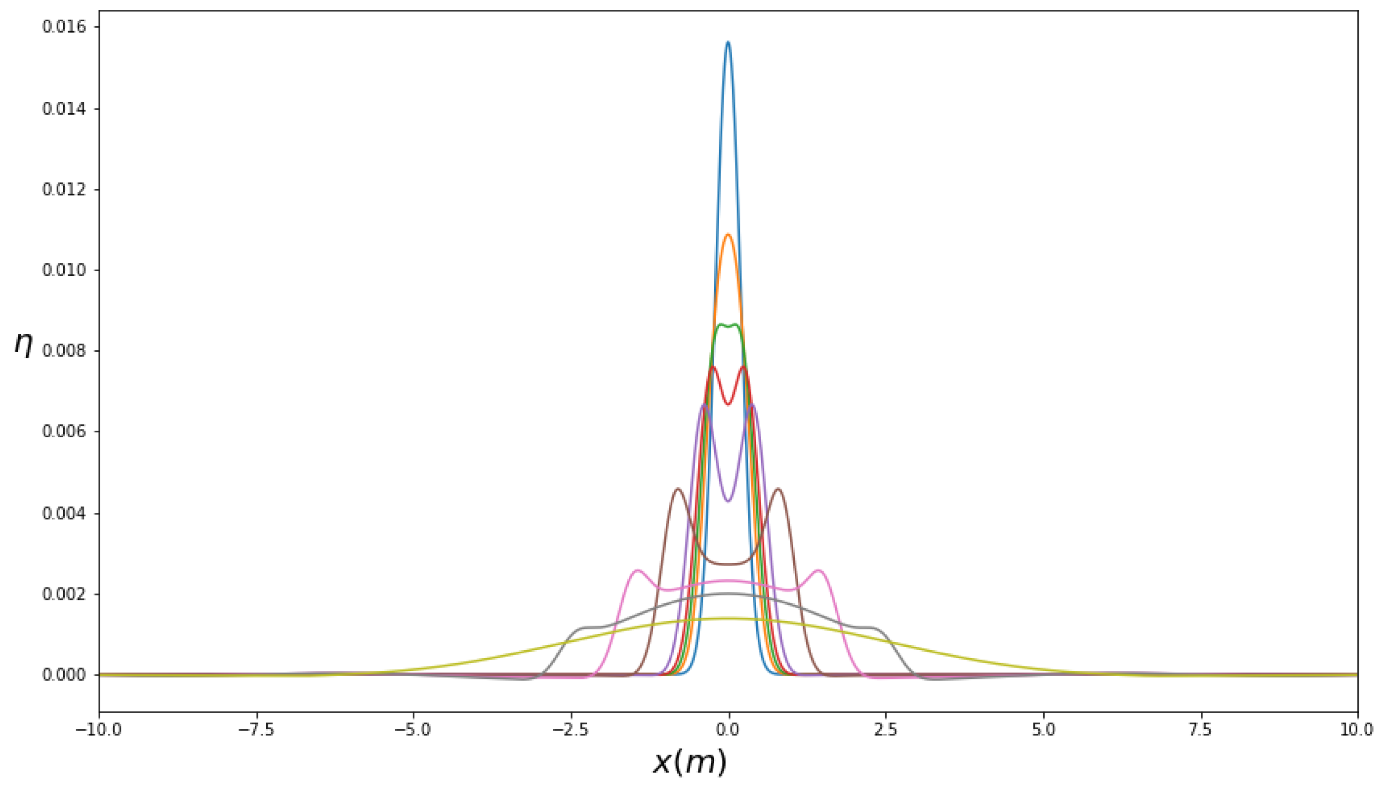
As an application of Equations (100)–(107), a narrow initial Gaussian profile (blue line) encompassing both propagating modes and over-damped modes is chosen (cf. Figure 19). Time evolution can be seen on the displayed profiles with different colours.
It is seen that the two peaks develop and radiate off symmetrically due to the propagating modes. Since there is no initial velocity, the peaks are in the same weight. Gradually, the Gaussian wave gives way to a much broader Gaussian shape profile, composed of non-propagating over-damped modes (yellow line). It is worth mentioning that in this example over-damped modes have a much smaller damping rate than the propagating ones. Therefore, the contributions of the propagating modes, the peaks, decay, and the longer living over-damped mode content of the initial profile becomes visible.
7. Conclusions
Linear viscous capillary-gravity waves were studied in a channel of constant depth, without restricting the parameters. The resulting dispersion relation is published for the first time. We explored all the modes numerically. Modes were labelled by horizontal wave number K, a continuous parameter, and vertical wave number Q, a discrete, complex quantity. We found that there were always infinitely many non-propagating (over-damped) modes. Propagation can only occur in the two modes with the smallest decay. In a sufficiently thin layer no propagation occurs at all. When increasing layer thickness, a bifurcation occurs, which shows up in the plot of imaginary parts of frequencies, such as a collision of the lowest lying branches of modes. After that collision, at increasing wave numbers, one can observe a merging and a subsequent split of these branches. The wave number range of the merged section frequencies have a non-zero real part (propagation). We stress that even at those depths where propagation becomes possible, propagation at very low and very high wave numbers is still prohibited. The over-damping at large wave numbers is already known [21,37]. The over-damping at small wave numbers has been discussed in Section 2.4. This is due to the fact that by increasing the wavelength, the restoring force (due to gravity) does not change, but the friction increases significantly. We also determined the minimal layer thickness necessary for wave propagation. Further, we studied surface motion. Assuming a monochromatic wave propagating to the positive x direction, we found that a surface particle in a viscous fluid could rotate both clockwise or counterclockwise, depending on the wave number. We also demonstrated the propagation or non-propagation of waves in a few cases. In order to illustrate that both positive, zero, or even negative group velocities can occur, the beat of two nearby wave numbers was displayed at a few consecutive time instants. Finally, with the assumption that the effect of fast decaying high lying branches was negligible, we kept the lowest two modes and formulated the solution of the initial value problem of surface motion in wave number space. As an application, the time evolution of a narrow initial Gaussian surface elevation with zero velocity was studied and a radiation of propagating modes in the form of two oppositely travelling bumps was observed. A slowly decaying wide Gaussian was left behind, consisting of large wavelength non-propagating modes.
It is remarkable how many interesting phenomena occur in this simple setup. It is an intriguing question what happens in the presence of an elastic surface at finite fluid depth, since two propagation modes, a capillary mode and a dilational mode, exist in deep water [23].
It is a natural question whether and how these results can have practical applications. As we already noted, in water most of the phenomena discussed are unobservable, because its viscosity is small and surface tension is large. In thick oils, however, these phenomena might be observed. For actual applications (industrial, or perhaps biological) one has to consider thin layers, but then other surface effects, such as pollution or surface elasticity, should be included, as well. It is tempting to think of the effect of the surfactant because they clearly decrease surface tension and with that . However, with surfactants a wealth of new phenomena appear, e.g., the possibility of a dilational wave due to the presence of surface elasticity and interplay between this propagating mode with capillary waves (cf. [21,23,47]). Such phenomena are certainly not covered by the current paper.
Another potential application might be in geology (lava flows, glaciers) with especially large viscosity or planetology with different g parameters. In the first case, however, many other effects can be important, too, so the results of the present work could be used as the order of magnitude estimates at best. In case of other planets, a larger g decreases , since it is proportional to , but at the same time parameter p is decreased, so an even thinner fluid layer (or larger viscosity) is necessary to prevent wave propagation, than in Earth. However, the minimal layer thickness was determined numerically, so it is not straightforward to predict the effect of changing g. It may happen that under suitable planetary circumstances the minimal layer thickness for some fluid that is present in abundance will be significantly larger than that for water on Earth.
Author Contributions
Conceptualization, A.G. and G.B.; methodology, A.G. and G.B.; formal analysis, A.G. and G.B.; investigation, A.G. and G.B.; writing—original draft preparation, A.G. and G.B.; writing—review and editing, A.G. and G.B.; visualization, A.G. and G.B.; supervision, G.B. All authors have read and agreed to the published version of the manuscript.
Funding
This research received no external funding.
Acknowledgments
This research was supported by the Ministry of Culture and Innovation and the National Research. A.G. greatly acknowledges the support from Stipendium Hungaricum. We are indebted to our reviewers for their many helpful comments and suggestions.
Conflicts of Interest
The authors declare no conflict of interest.
References
- Naeser, H. The Capillary Waves’ Contribution to Wind-Wave Generation. Fluids 2022, 7, 73. [Google Scholar] [CrossRef]
- Berhanu, M. Impact of the dissipation on the nonlinear interactions and turbulence of gravity-capillary waves. Fluids 2022, 7, 137. [Google Scholar] [CrossRef]
- Gnevyshev, V.; Badulin, S. Wave patterns of gravity–capillary waves from moving localized sources. Fluids 2020, 5, 219. [Google Scholar] [CrossRef]
- Bongarzone, A.; Gallaire, F. Numerical estimate of the viscous damping of capillary-gravity waves: A macroscopic depth-dependent slip-length model. arXiv 2022, arXiv:2207.06907. [Google Scholar]
- Behroozi, F.; Smith, J.; Even, W. Effect of viscosity on dispersion of capillary–gravity waves. Wave Motion 2011, 48, 176–183. [Google Scholar] [CrossRef]
- Lu, D.; Ng, C.O. Interfacial capillary–gravity waves due to a fundamental singularity in a system of two semi-infinite fluids. J. Eng. Math. 2008, 62, 233–245. [Google Scholar] [CrossRef]
- Denner, F.; Gounsetti, P.; Zaleski, S. Dispersion and viscous attenuation of capillary waves with finite amplitude. HAL 2017, 226, 1229–1238. [Google Scholar] [CrossRef]
- Shen, L.; Denner, F.; Morgan, N.; van Wachem, B.; Dini, D. Marangoni effect on small-amplitude capillary waves in viscous fluids. Phys. Rev. E 2017, 96, 053110. [Google Scholar] [CrossRef]
- Kim, N.; Debnath, L. Motion of a buoy on weakly viscous capillary gravity waves. Int. J. Nonlinear Mech. 2000, 35, 405–420. [Google Scholar] [CrossRef]
- Lu, D.Q. Analytical solutions for the interfacial viscous capillary-gravity waves due to an oscillating Stokeslet. J. Hydrodyn. 2019, 31, 1139–1147. [Google Scholar] [CrossRef]
- Young, I.R.; Babanin, A.V. Spectral distribution of energy dissipation of wind-generated waves due to dominant wave breaking. J. Phys. Oceanogr. 2006, 36, 376–394. [Google Scholar] [CrossRef]
- Babanin, A.; Young, I. Two-phase behaviour of the spectral dissipation of wind waves. In Proceedings of the 5th International Symposium Ocean Wave Measurement and Analysis, Madrid, Spain, 3–7 July 2005. [Google Scholar]
- Sutherland, B.R.; Balmforth, N.J. Damping of surface waves by floating particles. Phys. Rev. Fluids 2019, 4, 014804. [Google Scholar] [CrossRef]
- Sutherland, B.R. Finite-amplitude internal wavepacket dispersion and breaking. J. Fluid Mech. 2001, 429, 343–380. [Google Scholar] [CrossRef]
- Babanin, A.V.; Tsagareli, K.N.; Young, I.; Walker, D.J. Numerical investigation of spectral evolution of wind waves. Part II: Dissipation term and evolution tests. J. Phys. Oceanogr. 2010, 40, 667–683. [Google Scholar] [CrossRef]
- Lamb, H. Hydrodynamics; Cambridge University Press: Cambridge, UK, 1924. [Google Scholar]
- Ermakov, S.; Sergievskaya, I.; Gushchin, L. Damping of gravity-capillary waves in the presence of oil slicks according to data from laboratory and numerical experiments. Izv. Atmos. Ocean. Phys. 2012, 48, 565–572. [Google Scholar] [CrossRef]
- Rajan, G.K. A three-fluid model for the dissipation of interfacial capillary-gravity waves. Phys. Fluids 2020, 32, 122121. [Google Scholar] [CrossRef]
- Rajan, G.K. Damping rate measurements and predictions for gravity waves in an air–oil–water system. Phys. Fluids 2022, 34, 022113. [Google Scholar] [CrossRef]
- Kalinichenko, V. Standing Gravity Waves on the Surface of a Viscous Liquid. Fluid Dyn. 2022, 57, 891–899. [Google Scholar] [CrossRef]
- Rajan, G.K. Solutions of a comprehensive dispersion relation for waves at the elastic interface of two viscous fluids. Eur. J. Mech. B Fluids 2021, 89, 241–258. [Google Scholar] [CrossRef]
- Sergievskaya, I.; Ermakov, S. Damping of gravity–capillary waves on water surface covered with a visco-elastic film of finite thickness. Izv. Atmos. Ocean. Phys. 2017, 53, 650–658. [Google Scholar] [CrossRef]
- Earnshaw, J.; McLaughlin, A. Waves at liquid surfaces: Coupled oscillators and mode mixing. Proc. R. Soc. Lond. Ser. A Math. Phys. Sci. 1991, 433, 663–678. [Google Scholar]
- Lucassen-Reynders, E.; Lucassen, J. Properties of capillary waves. Adv. Colloid Interface Sci. 1970, 2, 347–395. [Google Scholar] [CrossRef]
- Denner, F. Frequency dispersion of small-amplitude capillary waves in viscous fluids. Phys. Rev. E 2016, 94, 023110. [Google Scholar] [CrossRef]
- Shen, L.; Denner, F.; Morgan, N.; van Wachem, B.; Dini, D. Capillary waves with surface viscosity. J. Fluid Mech. 2018, 847, 644–663. [Google Scholar] [CrossRef]
- Sauleda, M.L.; Hsieh, T.L.; Xu, W.; Tilton, R.D.; Garoff, S. Surfactant spreading on a deep subphase: Coupling of Marangoni flow and capillary waves. J. Colloid Interface Sci. 2022, 614, 511–521. [Google Scholar] [CrossRef]
- Delgado-Buscalioni, R.; Chacon, E.; Tarazona, P. Hydrodynamics of nanoscopic capillary waves. Phys. Rev. Lett. 2008, 101, 106102. [Google Scholar] [CrossRef]
- Bühler, O. Waves and Mean Flows; Cambridge University Press: Cambridge, UK, 2014. [Google Scholar]
- Rajan, G.K.; Henderson, D.M. The linear stability of a wavetrain propagating on water of variable depth. SIAM J. Appl. Math. 2016, 76, 2030–2041. [Google Scholar] [CrossRef]
- Sergievskaya, I.; Ermakov, S.; Lazareva, T.; Guo, J. Damping of surface waves due to crude oil/oil emulsion films on water. Mar. Pollut. Bull. 2019, 146, 206–214. [Google Scholar] [CrossRef]
- Sergievskaya, I.; Ermakov, S. A phenomenological model of wave damping due to oil films. In Proceedings of the Remote Sensing of the Ocean, Sea Ice, Coastal Waters, and Large Water Regions 2019, Strasbourg, France, 9–10 September 2019; Volume 11150, pp. 153–158. [Google Scholar]
- Henderson, D.M.; Segur, H. The role of dissipation in the evolution of ocean swell. J. Geophys. Res. Ocean. 2013, 118, 5074–5091. [Google Scholar] [CrossRef]
- Henderson, D.; Miles, J. Surface-wave damping in a circular cylinder with a fixed contact line. J. Fluid Mech. 1994, 275, 285–299. [Google Scholar] [CrossRef]
- Henderson, D.M. Effects of surfactants on Faraday-wave dynamics. J. Fluid Mech. 1998, 365, 89–107. [Google Scholar] [CrossRef]
- Le Meur, H.V. Derivation of a viscous Boussinesq system for surface water waves. Asymptot. Anal. 2015, 94, 309–345. [Google Scholar] [CrossRef]
- Armaroli, A.; Eeltink, D.; Brunetti, M.; Kasparian, J. Viscous damping of gravity-capillary waves: Dispersion relations and nonlinear corrections. Phys. Rev. Fluids 2018, 3, 124803. [Google Scholar] [CrossRef]
- Hunt, J. The viscous damping of gravity waves in shallow water. Houille Blanche 1964, 6, 685–691. [Google Scholar] [CrossRef]
- Sanochkin, Y.V. Viscosity effect on free surface waves in fluids. Fluid Dyn. 2000, 35, 599–604. [Google Scholar] [CrossRef]
- Lucassen, J. Longitudinal capillary waves. Part 1.—Theory. Trans. Faraday Soc. 1968, 64, 2221–2229. [Google Scholar] [CrossRef]
- Kramer, L. Theory of light scattering from fluctuations of membranes and monolayers. J. Chem. Phys. 1971, 55, 2097–2105. [Google Scholar] [CrossRef]
- Biesel, F. Calculation of wave damping in a viscous liquid of known depth. Houille Blanche 1949, 4, 630–634. [Google Scholar] [CrossRef]
- Baldi, P.; Toland, J.F. Steady Periodic Water Waves under Nonlinear Elastic Membranes; De Gruyter: Berlin, Germany, 2011. [Google Scholar]
- Baldi, P.; Toland, J.F. Bifurcation and secondary bifurcation of heavy periodic hydroelastic travelling waves. Interfaces Free Boundaries 2010, 12, 1–22. [Google Scholar] [CrossRef]
- Toland, J.F.; Jones, M. The bifurcation and secondary bifurcation of capillary-gravity waves. Proc. R. Soc. Lond. A Math. Phys. Sci. 1985, 399, 391–417. [Google Scholar]
- Jones, M.T.J. Symmetry and the bifurcation of capillary-gravity waves. Arch. Ration. Mech. Anal. 1986, 96, 29–53. [Google Scholar] [CrossRef]
- Brown, S.; Triantafyllou, M.; Yue, D. Complex analysis of resonance conditions for coupled capillary and dilational waves. Proc. R. Soc. Lond. Ser. A Math. Phys. Eng. Sci. 2002, 458, 1167–1187. [Google Scholar] [CrossRef]
- Constantin, A.; Varvaruca, E. Steady periodic water waves with constant vorticity: Regularity and local bifurcation. Arch. Ration. Mech. Anal. 2011, 199, 33–67. [Google Scholar] [CrossRef]
- Martin, C.I. Local bifurcation for steady periodic capillary water waves with constant vorticity. J. Math. Fluid Mech. 2013, 15, 155–170. [Google Scholar] [CrossRef]
Figure 1.
First, we find 10 branches of solutions for glycerin at . The majority of the frequencies remain purely imaginary, but the two lowest branches intersect when the value of K is increased.
Figure 1.
First, we find 10 branches of solutions for glycerin at . The majority of the frequencies remain purely imaginary, but the two lowest branches intersect when the value of K is increased.

Figure 2.
Two lowest branches of solutions for glycerin at different p values. Moduli of imaginary parts of frequencies are displayed. (a) Two lowest branches of solutions for glycerin at . (b) Two lowest branches of solutions for glycerin at . (c) Two lowest branches of solutions for glycerin at . The collision no longer occurs by increasing the value of p.

Figure 3.
The real and imaginary parts of frequencies corresponding to the lowest lying branches versus K for glycerin at cm).
Figure 3.
The real and imaginary parts of frequencies corresponding to the lowest lying branches versus K for glycerin at cm).

Figure 7.
Motion of the particles at the surface.

Figure 8.
The ratio of and the angles and in terms of K are presented for glycerin at (cf. Figure 3). Angles are given in units.
Figure 8.
The ratio of and the angles and in terms of K are presented for glycerin at (cf. Figure 3). Angles are given in units.

Figure 9.
Time evolution of surface elevation in glycerin at parameter and wave number .

Figure 10.
Time evolution of surface elevation in glycerin at parameter and wave number .

Figure 11.
Time evolution of surface elevation in glycerin at parameter and wave number .

Figure 12.
Time evolution of surface elevation in glycerin at parameter and wave number .

Figure 13.
Time evolution of surface elevation in glycerin at parameter and wave number .

Figure 14.
Time evolution of surface elevation in glycerin at parameter and wave number .

Figure 15.
Time evolution of surface elevation in glycerin at parameter and wave number .

Figure 16.
Time evolution of surface elevation in glycerin at parameter with two nearby wave numbers at ().
Figure 16.
Time evolution of surface elevation in glycerin at parameter with two nearby wave numbers at ().

Figure 17.
Time evolution of surface elevation in glycerin at parameter with two nearby wave numbers at ().
Figure 17.
Time evolution of surface elevation in glycerin at parameter with two nearby wave numbers at ().

Figure 18.
Time evolution of surface elevation in glycerin at parameter with two nearby wave numbers at ().
Figure 18.
Time evolution of surface elevation in glycerin at parameter with two nearby wave numbers at ().

Figure 19.
Time evolution of an initial Gaussian wave for glycerin at presented. Time values are t = 0., 0.3, 0.4, 0.5, 0.7, 1.4, 2.5, 4, and 10 s. A slim initial Gaussian wave (blue line) containing both propagating modes and over-damped modes spreads outwards and gradually diminishes and leaves behind a broader Gaussian shape profile due to non-propagating modes at long wavelengths (yellow line).


Table 1.
Material parameters , and for some fluids.
| Material | h | ||||
|---|---|---|---|---|---|
| water | 58.40 | ||||
| glycerin | 0.45 1 | 0.085 | |||
| mercury | 174.86 |
1 Properties are at 20 °C.
Disclaimer/Publisher’s Note: The statements, opinions and data contained in all publications are solely those of the individual author(s) and contributor(s) and not of MDPI and/or the editor(s). MDPI and/or the editor(s) disclaim responsibility for any injury to people or property resulting from any ideas, methods, instructions or products referred to in the content. |
© 2023 by the authors. Licensee MDPI, Basel, Switzerland. This article is an open access article distributed under the terms and conditions of the Creative Commons Attribution (CC BY) license (https://creativecommons.org/licenses/by/4.0/).
Share and Cite
MDPI and ACS Style
Ghahraman, A.; Bene, G. Bifurcation Analysis and Propagation Conditions of Free-Surface Waves in Incompressible Viscous Fluids of Finite Depth. Fluids 2023, 8, 173. https://doi.org/10.3390/fluids8060173
AMA Style
Ghahraman A, Bene G. Bifurcation Analysis and Propagation Conditions of Free-Surface Waves in Incompressible Viscous Fluids of Finite Depth. Fluids. 2023; 8(6):173. https://doi.org/10.3390/fluids8060173
Chicago/Turabian StyleGhahraman, Arash, and Gyula Bene. 2023. "Bifurcation Analysis and Propagation Conditions of Free-Surface Waves in Incompressible Viscous Fluids of Finite Depth" Fluids 8, no. 6: 173. https://doi.org/10.3390/fluids8060173