
Modelling Time-Dependent Flow through Railway Ballast


1
School of Information and Physical Sciences, The University of Newcastle, Callaghan, NSW 2308, Australia
2
Department of Mathematics, Jamoum University College, Umm Al-Qura University, Jamoum, Makkah 21955, Saudi Arabia
*
Author to whom correspondence should be addressed.
Fluids 2023, 8(6), 170; https://doi.org/10.3390/fluids8060170
Submission received: 8 March 2023
/
Revised: 20 May 2023
/
Accepted: 25 May 2023
/
Published: 31 May 2023
Abstract
:In this study, a numerical simulation of fluid flow through railway ballast in the time domain is presented, providing a model for unsteady-state flow. It is demonstrated that the position of the free surface with respect to time can also be used to solve the steady flow case. The effect of ballast fouling is included in the model to capture the realistic behavior of railway ballast, which is critical to understanding the impact of flooding. A thorough comparison with a range of previous studies, including theoretical and experimental approaches, is made, and very close agreement is obtained. The significant impact of ballast fouling on fluid flow and its potential consequences for railway infrastructure are highlighted by the simulation. Valuable insights into the behavior of water flow through porous media and its relevance to railway ballast management are offered by this study.
1. Introduction
The understanding of water flow behavior through porous media is crucial in many applications to minimize damage caused by seepage [1,2,3,4,5]. In this context, the present study focuses on water flow through railway ballast, which is commonly modeled as a porous medium. Of particular importance is the scouring of railway ballast due to flood waters, which can occur when the upstream height exceeds the railway ballast’s height [6,7]. Heterogeneous ballast gradations can also cause erosion of the ballast, even if the upstream height is less than the railway ballast’s height [8]. The scouring of railway ballast can lead to catastrophic outcomes, as discussed in [9], particularly if the ballast becomes too weak to support the weight of a train.
However, analyzing the problem of porous media flow is much more challenging when the free surface needs to be calculated. The problem becomes even more complicated when considering the time-dependent motion of the problem. Nevertheless, solving the time-dependent problem, which involves determining the free surface position of water flow, can be used to provide the steady-state solution (which is commonly calculated iteratively) [10]. In our present study, we also use the method developed to solve for the steady-state unknown free surface.
Nonetheless, the primary challenge is to solve the unsteady problem, where the actual time is considered. This problem represents the realistic flow through porous media and the time-dependent change in the position of the free surface. We must also consider the specific yield when investigating the motion of the free surface for unsteady flow, whereas this is not necessary for determining the steady-state solution [10]. The specific yield models the drainage capacity of the porous material [11]. In the present work, we particularly focus on validating our calculations by comparing them with results in the literature, particularly those obtained from three cases in [12,13], in which they solved for the steady-state flow through a rectangular dam. For the unsteady calculations, we use the experimental results calculated in [14] and the theoretical results of [15].
The aim of this work is to develop numerical methods to determine the unsteady flow through railway ballast with a moving free boundary. We consider realistic ballast models that represent the effect of ballast fouling, which is regarded as critical to ballast flooding. We also thoroughly and carefully validate our present study by comparing it with previous studies [12,13,14,15] and our previous study [9], which solved the steady free boundary problem. We use the Finite Element Method (FEM) for all our calculations.
2. Methods and Numerical Modeling of Flow through Ballast
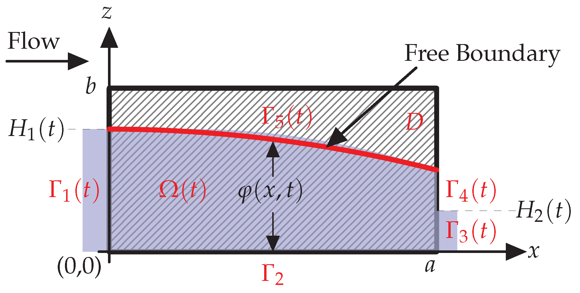
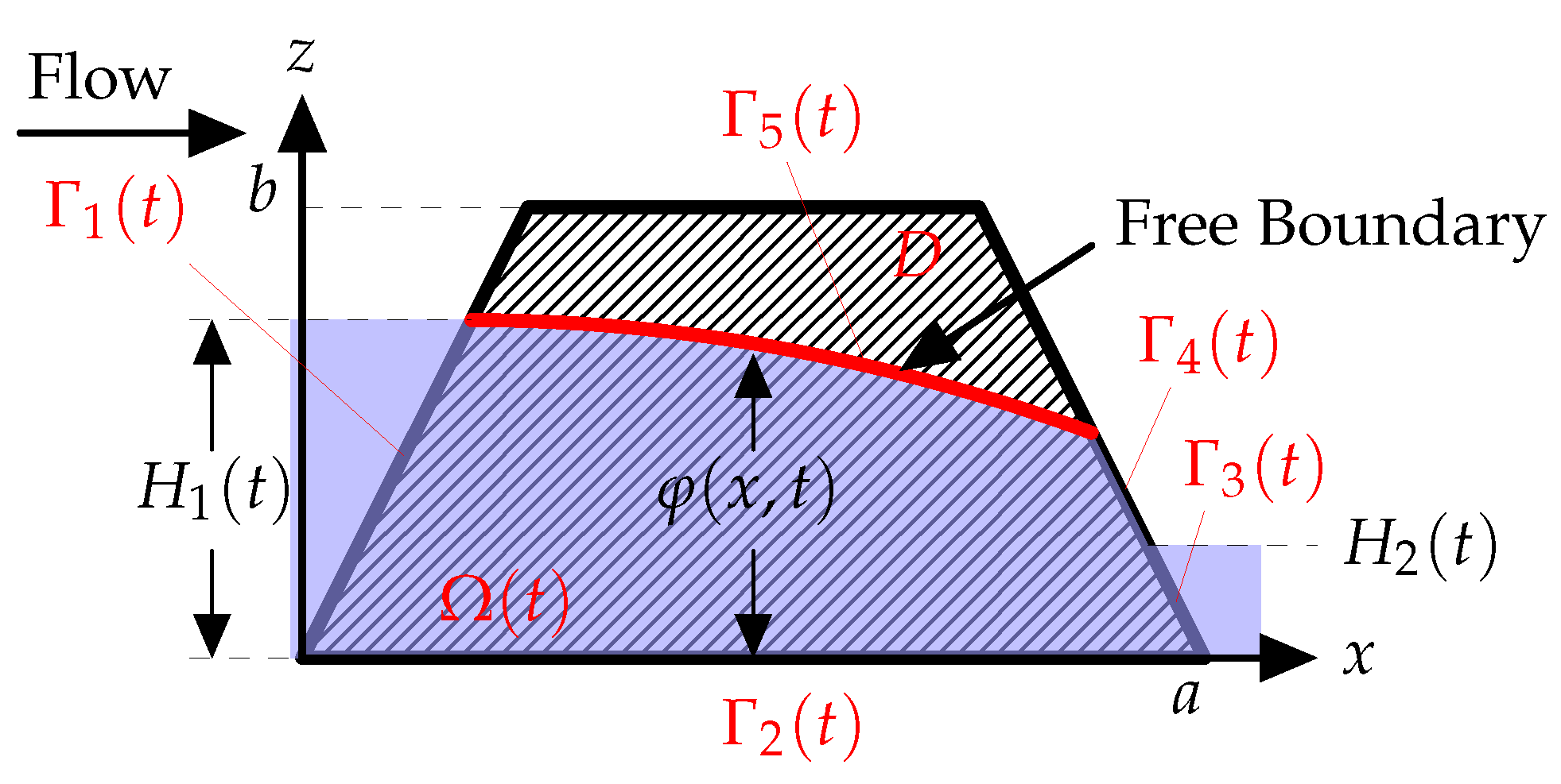
The region under consideration is depicted in Figure 1 and can be defined by the domain . The saturated part of the region is denoted by , which is a function of time t, where . Here, represents the water level inside the rectangular ballast. The free surface within the porous medium is denoted by , while and represent the upstream and downstream regions, respectively, with a fluid boundary. The seepage face is denoted by . The water heights are represented by and , while the impermeable boundary is represented by , where there is no flux.
The governing equation is derived from the divergence of the seepage velocity and is given by
where and are the hydraulic conductivity and the hydraulic head, respectively [16]. We use the following boundary conditions [12]
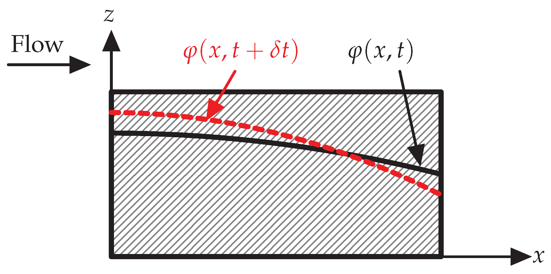
The final condition is that for the movement of the free surface,
where is the specific yield. We will discuss this term shortly. We also need to specify the initial value of the free surface
The solution of Equation (1) with boundary conditions (2) is obtained using the finite element method, as described in [16]. Time marching is employed to solve the boundary equation and track the movement of the free boundary over time:
in Ref. [12]. The movement of the free boundary function with respect to time is shown in Figure 2.
In order to investigate the effect of variable inflow levels on the unsteady-state flow, it is necessary to define the evolution of the water level with respect to time. The inclusion of the specific yield is important for our railway ballast problem [11], although not all previous studies have considered this term. Caution must be exercised when comparing our results with those reported in the literature. The importance of is discussed in [10]. The method for obtaining the free surface in Equation (4) by dividing hydraulic conductivity by the specific yield was developed by France et al. [17] and Mills [18]. This method does not have any impact on the numerical difficulties encountered. Unless explicitly stated otherwise, we will assume to be unity.
3. Results for Rectangular Regions
We will commence by examining the three cases that have been previously explored by [12,13], in which the inflow height is constant for all three. We will compute these three cases and conduct a thorough comparison with the aforementioned studies. The specific parameters for each case are outlined in Table 1.
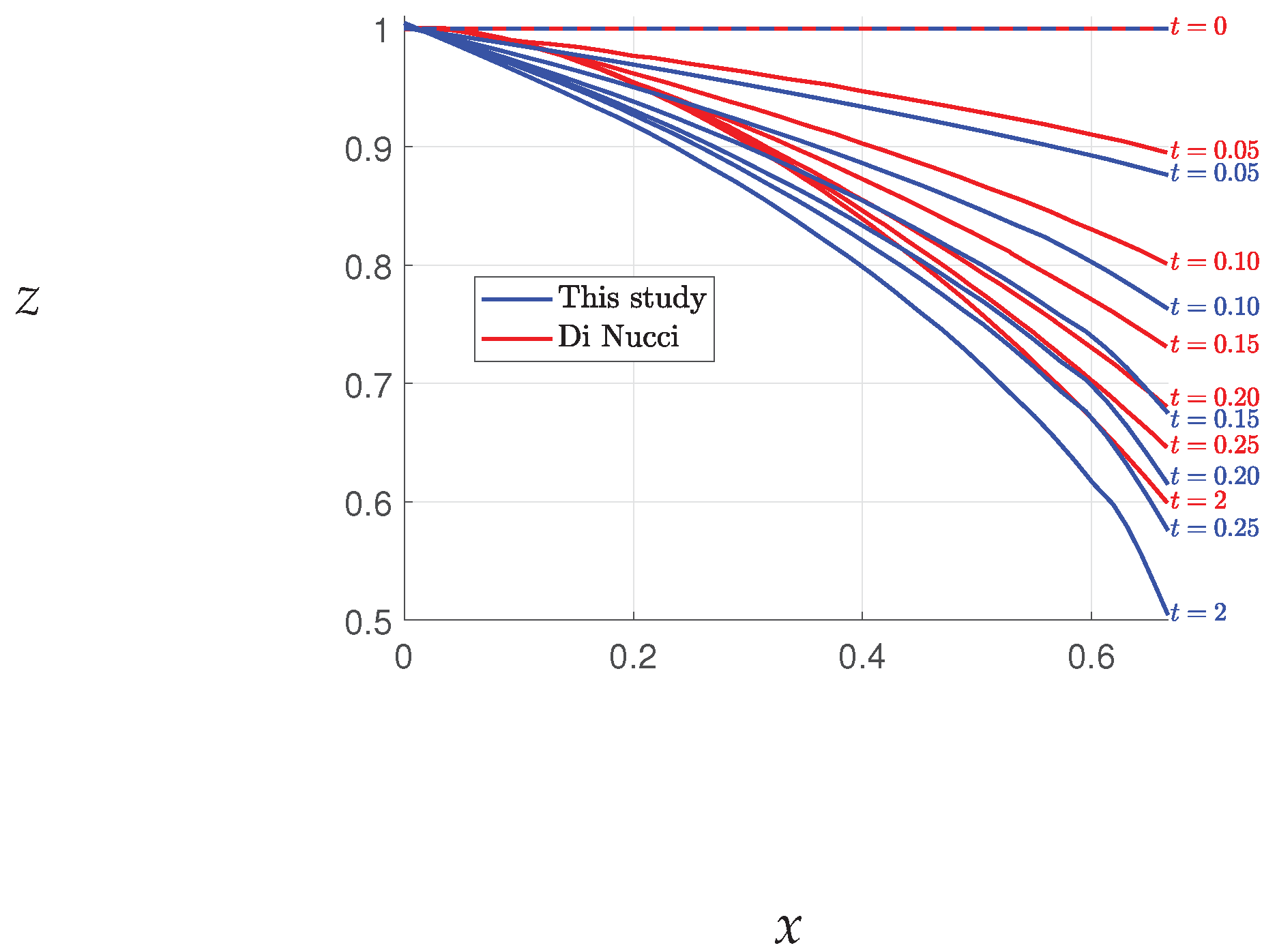
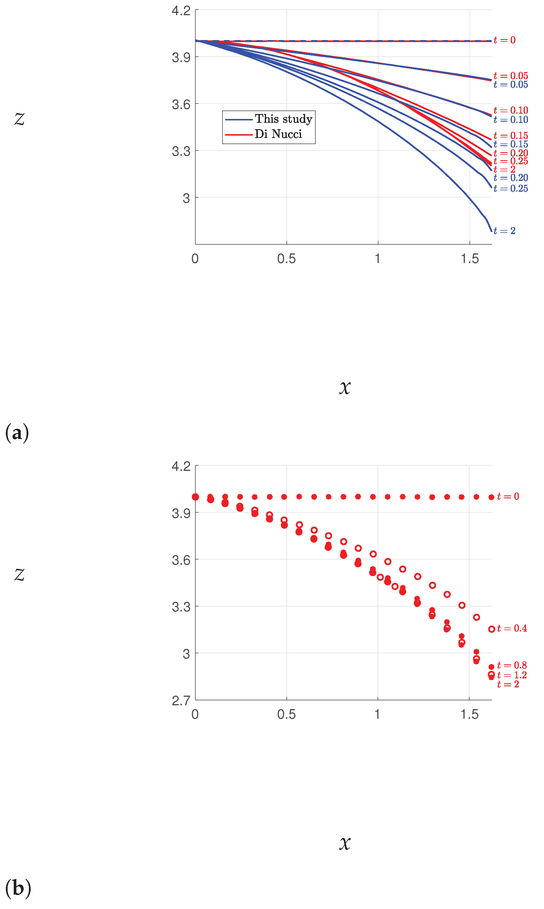
The results of Case 1 are presented in Figure 3, where the free surface elevations obtained with our method are compared with those obtained by Di Nucci [13], who employed an approximate method to solve the same problem. A slight discrepancy between the free surface elevations is observed, with Di Nucci’s results yielding higher elevations than ours. However, such a difference is not surprising given that the two methods solve slightly different problems. Conversely, the results of Chakib and Nachaoui [12], depicted in Figure 4, exhibit discrepancies with our outcomes, as shown in Figure 3. Nonetheless, our results match closely with those of Di Nucci, as previously mentioned. We also note that our final free surface elevations align with those of Chakib and Nachaou, as depicted in Figure 5. We thus infer that the errors in Chakib and Nachaou’s outcomes stem from their time steps, while the consistency of our results with Di Nucci’s supports the accuracy of our method.
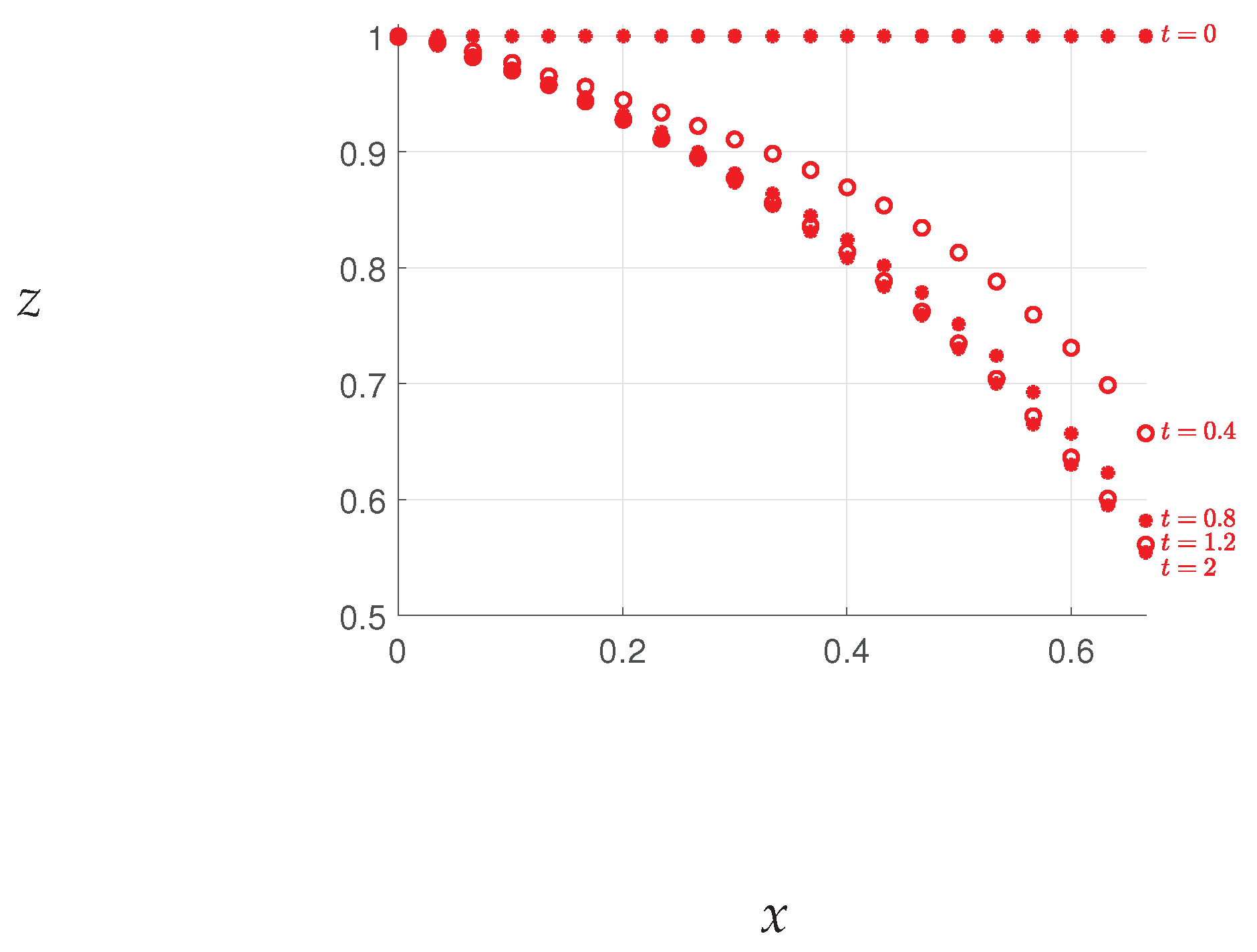
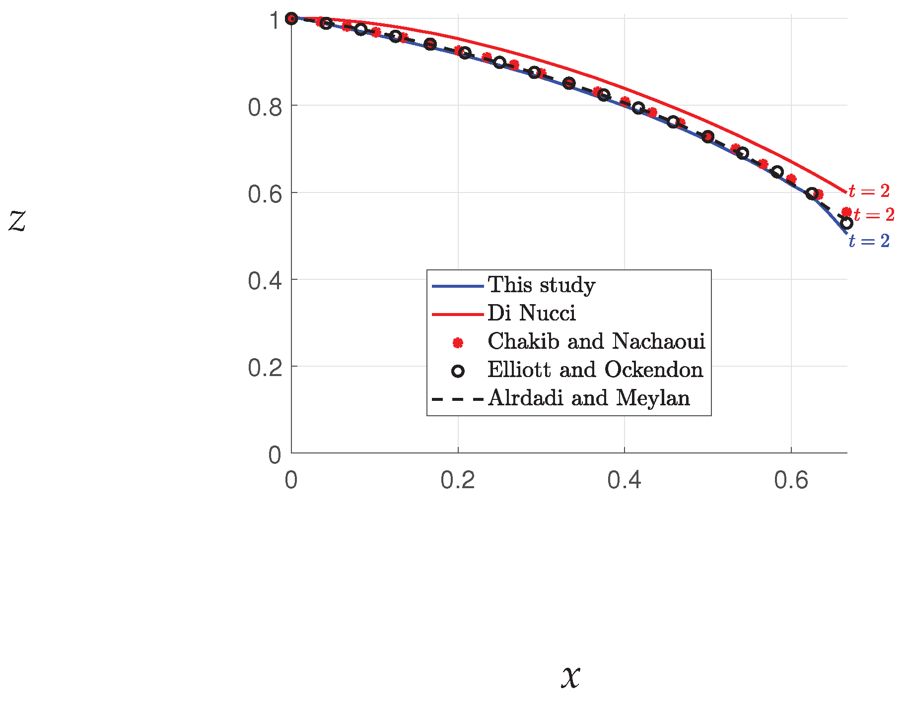
The results obtained for Case 1 enable a comparison of the free surface evolution, as shown in Figure 5. The figure includes the free surface results from this study, as well as those from previous investigations, including the steady-state results reported in [16,19]. Figure 6 displays the free surface convergences at over the time interval , as well as the steady-state free surface. The variation in is relatively constant for in both this study and Di Nucci’s study, while Chakib and Nachaoui’s study shows a slightly different pattern, with the variation in being constant for , as evident from Figure 6. The solution converges to the desired accuracy when , as illustrated in Figure 5 and Figure 6.
The free surface elevations for Cases 2 and 3 are presented in Figure 7 and Figure 8, respectively. The steady-state free surface solutions for these cases are computed through the iterative algorithm proposed in [9]. Our findings indicate that the results and conclusions for Cases 2 and 3 are comparable to those of Case 1.
3.1. Unsteady-State Flow through a Rectangular Dam
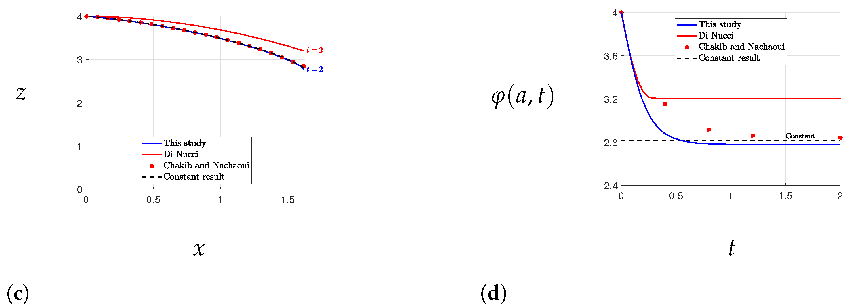
In this study, we compare our results with the findings reported in [15] concerning the flow of water through a homogeneous rectangular dam with a hydraulic conductivity of 1 m/s. The dam dimensions are 500 m in width and 12 m in height. In this scenario, the inflow water level rises abruptly from an equilibrium value of 7 m to 12 m at the first time step. The time steps used in this case are half an hour. This case simulates a sudden flow through saturated railway ballast.
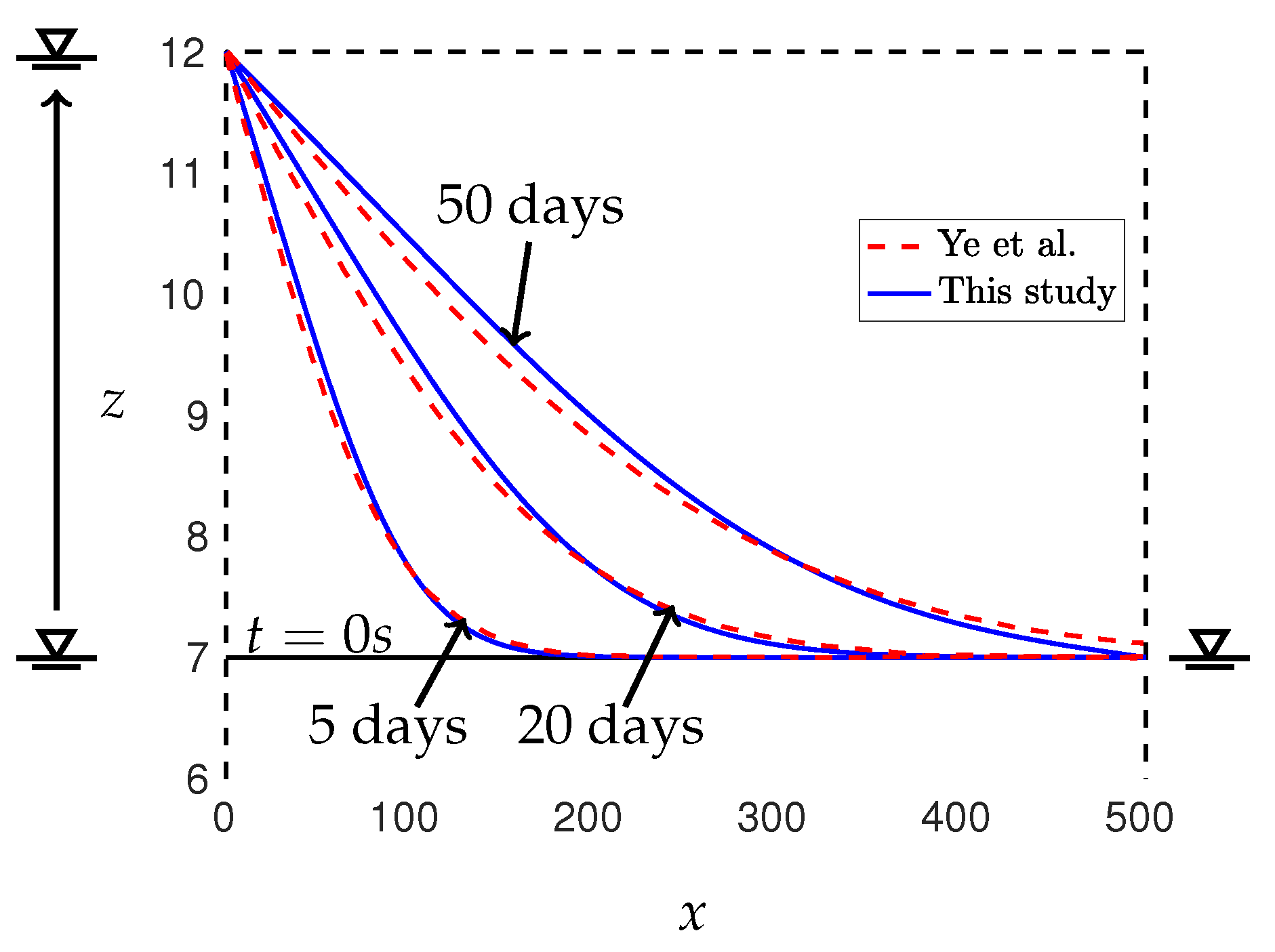
Figure 9 displays the solutions for the free surface of a rectangular dam with a specific yield of 0.1 at different times. The dam has a width of 500 m and a height of 12 m, with a hydraulic conductivity equal to 1 m/s. Additionally, we included the analytical solutions of Ye et al. [15] to compare them with the solutions from our method. The free-surface elevations were computed at , days, days, and days using a time step of half an hour. Our results exhibit excellent agreement with those of Zuyang et al. [15]. The calculations for various time steps are presented in Figure 10. This figure demonstrates that both time step values yield the same outcomes for the free-surface position. Selecting a higher value for during the calculation may cause a numerical instability error. Therefore, it is essential to choose an appropriate time step value to ensure good convergence. This issue is comprehensively discussed in Appendix A.
3.2. Unsteady-State Flow through a Trapezoidal Dam
The porous medium of railway ballast can be accurately modeled as trapezoidal in shape. In this study, we aim to analyze the unsteady-state flow through such a trapezoidal porous region. To achieve this, we apply the same boundary conditions as presented in Equation (2) but adapted to the trapezoidal shape, as depicted in Figure 11. The scenario under investigation involves a linear increase in the upstream variation, and the goal is to determine the free-surface position at different times. The obtained results will be carefully compared with previous studies in the field.
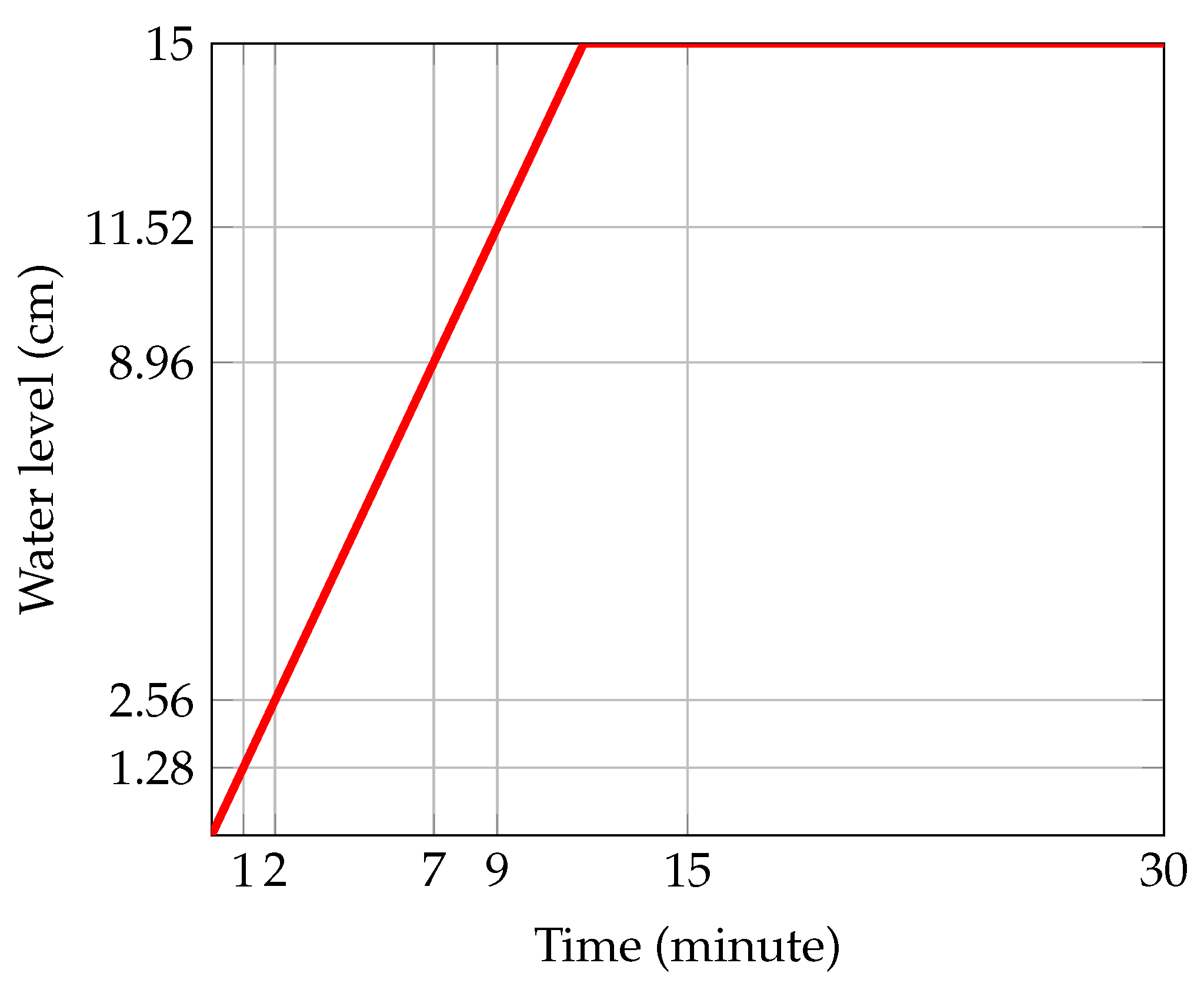
Desai et al. [14] conducted a comprehensive investigation of unsteady-state flow through various types of dams with differing hydraulic conductivities. Their study provides an opportunity to verify the validity of Equation (4) using diverse scenarios for the upstream variation. In one of their experiments, a trapezoidal dam was subjected to a linear increase in upstream head from 0 to 15 cm, as depicted in Figure 12. Analysis of the resulting increase in water level indicates a rate of increase of approximately cm/min, according to [15]. Thus, the water levels at 7 and 9 min were approximately cm and cm, respectively. This type of upstream variation mimics the flow of water through unsaturated railway ballast.
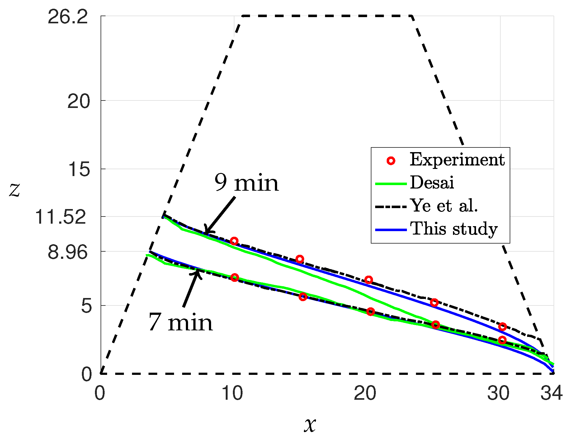
The experiment conducted by Desai et al. [14] involved a trapezoidal dam of 34 cm in length and 26.2 cm in height, with a hydraulic conductivity of 0.1 cm/s and a specific yield of 0.4. They recorded the free-surface elevations at 7 and 9 min. In this study, we aim to compare our predictions for the free-surface elevation of the saturated region of the dam with their experimental observations. Initially, we assume a straight line at a height of 3.84 cm, representing the water level at 3, and minimizing Equation (4) with , we determine the free surface. Our results, along with those of Desai et al. and Zuyang et al., are shown in Figure 13. The calculation of the free surface for this case is presented in Appendix B.
The results obtained from our analysis closely correspond with the experimental observations and the solutions proposed by Zuyang et al., as illustrated in Figure 13. While Desai et al.’s solution exhibited limitations after 9 min due to various factors that are discussed in [14], our method used a time step of , and we assumed a downstream height of cm as the boundary condition . It should be noted that the free-surface positions in our study are marginally lower downstream because of the maintenance of a downstream height of 0.05 cm. Consequently, we have established that our code is operational, and we have successfully completed the validation process.
4. Water Flow through Realistic Railway Ballast
4.1. Steady-State Flow for Realistic Railway Ballast
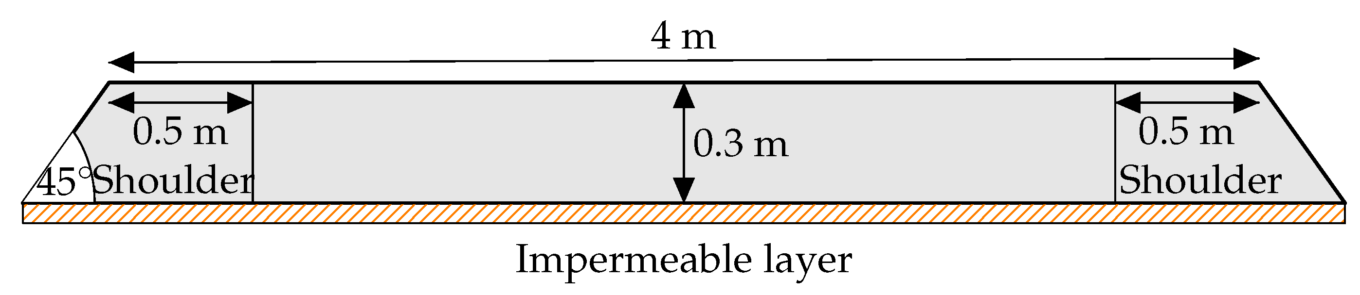
Here, we investigate the time-dependent water flow through railway ballast, taking into account the realistic dimensions of railway ballast, as depicted in Figure 14. Initially, we solve the steady-state flow problem and compare our results with the findings of [9]. We consider the porosity of the ballast to be affected by fouling, as illustrated in Figure 15, following the work of [9,20]. Subsequently, we analyze the free surface positions for various models, including clean ballast, Model 1, Model 2, and Model 3 (refer to Figure 15), as they evolve over time. The results are presented in Figure 17.
The red dashed lines presented in Figure 17 depict the free surface positions calculated using the iterative algorithm, as proposed in [9]. The time step, , used in all models was set to 0.05 s. Interestingly, each model resulted in different times for the final position of the free surface. For instance, the free surface of the clean ballast was achieved after 86.4 s, while for Models 1 and 2, it was achieved after 7 min. Our findings indicated that the free-surface positions for the first three models closely corresponded to those reported in [9]. However, in the last model, convergence was slower, and the iterative algorithm did not converge, even after 22 min.
The convergence rate of the time-dependent free surface in comparison to the steady-state free surface is significantly influenced by the hydraulic conductivity value, as demonstrated in Figure 17. The free surface of the clean ballast model converged at due to its homogeneous material with high conductivity. In contrast, Model 3 is nonhomogeneous and complex, with regions of low conductivity, resulting in a much slower convergence rate. Therefore, we suggest utilizing the iterative algorithm proposed in [9] for nonhomogeneous hydraulic conductivity, but only if the steady-state solution is required.
4.2. Unsteady-State Flow for Realistic Railway Ballast
In this section, we model a sudden flood in railway ballast by considering a sudden rise in water level upstream. We incorporate the specific yield to compute the free surface at various times. The specific yield represents the capacity of railway ballast to drain water. For realistic railway ballast, we assume a specific yield of 0.2, as coarse sand and gravel typically have specific yields of up to 0.2 [11]. We acknowledge that specific yield may vary with contamination, but we keep it constant at 0.2 for all models. We investigate the sudden flow for clean ballast and Model 1 in Figure 15, where the effect of the fouling ratio is similar to that depicted in Figure 16 for Model 1. We employ Equation (4) to determine the position of the free surface with respect to time. The hydraulic conductivity of the clean ballast is 0.3 m/s [9].
Figure 18 shows the results of our investigation on sudden flood scenarios for clean ballast and Model 1, where the sudden upstream change occurs from a stable water level height of 0.005 m to the height of the railway ballast of 0.3 m at the first time step of , while the downstream height is held constant at 0.005 m. We compared the free surface of both cases at specific time intervals of 0.1, 1, 5, 10, and 90 s. The impact of fouling in Model 1 greatly affected the free surface compared to the clean ballast case, in which the fouling ratio was considered. This effect is supported by previous studies on railway ballast scouring, which primarily occurs when the upstream height exceeds the height of the ballast [6,7]. We also observed that the ballast fouling in Model 1 led to a slower flow of water for a significant time compared to clean ballast, which may cause overflow in a continuous flooding situation.
5. Conclusions
The solution of time-dependent flow with a variable free surface in fluid flow through porous media is a powerful technique that enables the calculation of steady- and unsteady-state flows. In this study, we have investigated both flow these conditions and compared the results with experimental data. The steady-state flow results showed good agreement with the iterative algorithm proposed in [9], except in regions with highly variable hydraulic conductivity. For unsteady-state flow, we examined two inflow situations: linear and sudden increases. Specifically, we analyzed the latter case as it pertains to sudden floods that can occur in railway ballast. We demonstrated how fouling impacts the rate of water flow through ballast, as illustrated in Figure 18. Furthermore, we observed that the convergence of the free surface over time depends on the value of the specific yield, , for the unsteady state and that the time steps, , need to be chosen with care to obtain smooth curves for the free surface.
Author Contributions
Conceptualization, R.A. and M.H.M.; Methodology, M.H.M.; Investigation, R.A.; Writing—original draft, R.A.; Writing—review & editing, M.H.M.; Supervision, M.H.M.; Funding acquisition, M.H.M. All authors have read and agreed to the published version of the manuscript.
Funding
This research was funded by Australian Research Council’s Industrial Transformation Training Centres Scheme (ARC Training Centre for Advanced Technologies in Rail Track Infrastructure; IC170100006).
Data Availability Statement
Data is available by request.
Acknowledgments
This research was supported under Australian Research Council’s Industrial Transformation Training Centres Scheme (ARC Training Centre for Advanced Technologies in Rail Track Infrastructure; IC170100006).
Conflicts of Interest
The authors declare no conflict of interest.
Appendix A. Convergence Study of the Rectangular Dam for Steady-State Flow
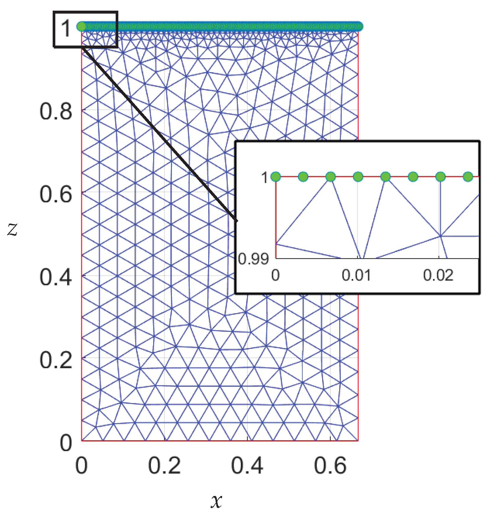
This section examines the computations employed in this study and outlines challenges encountered during the computation of the free surface. The finite element method requires the discretization of the domain into triangular sections, as depicted in Figure A1. Given that the flow near the free surface is highly variable, this section necessitates a higher number of elements. However, an excessive number of nodes may impede the iterative technique employed in updating the free surface.
Figure A1.
Mesh of case 1.

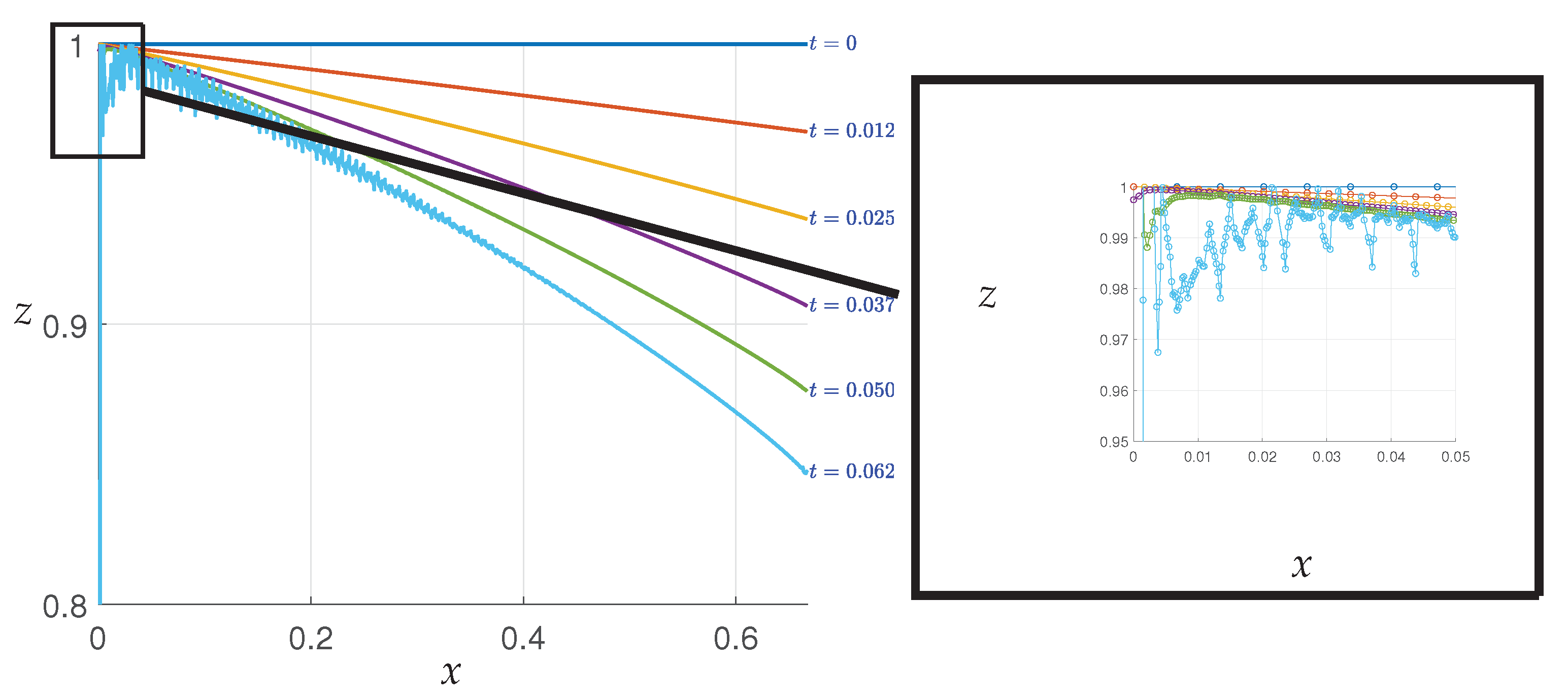
In Figure A2, it is observed that a high number of nodes made it difficult to converge the free boundary to the correct positions of the free surface. At s, variations in the free surface were detected, as shown in the figure. To facilitate the next convergence, it may be necessary to perturb the free surface at this point. One possible solution to this problem is to reduce the mesh density or the number of nodes on the free boundary (indicated by green nodes in Figure A1) to obtain the next free surface. However, a low mesh density can lead to inaccurate solutions. This issue was resolved in Figure A3, where the free surface became smooth.
Figure A2.
Errors caused by numerical instability, which appear as the time steps increase.

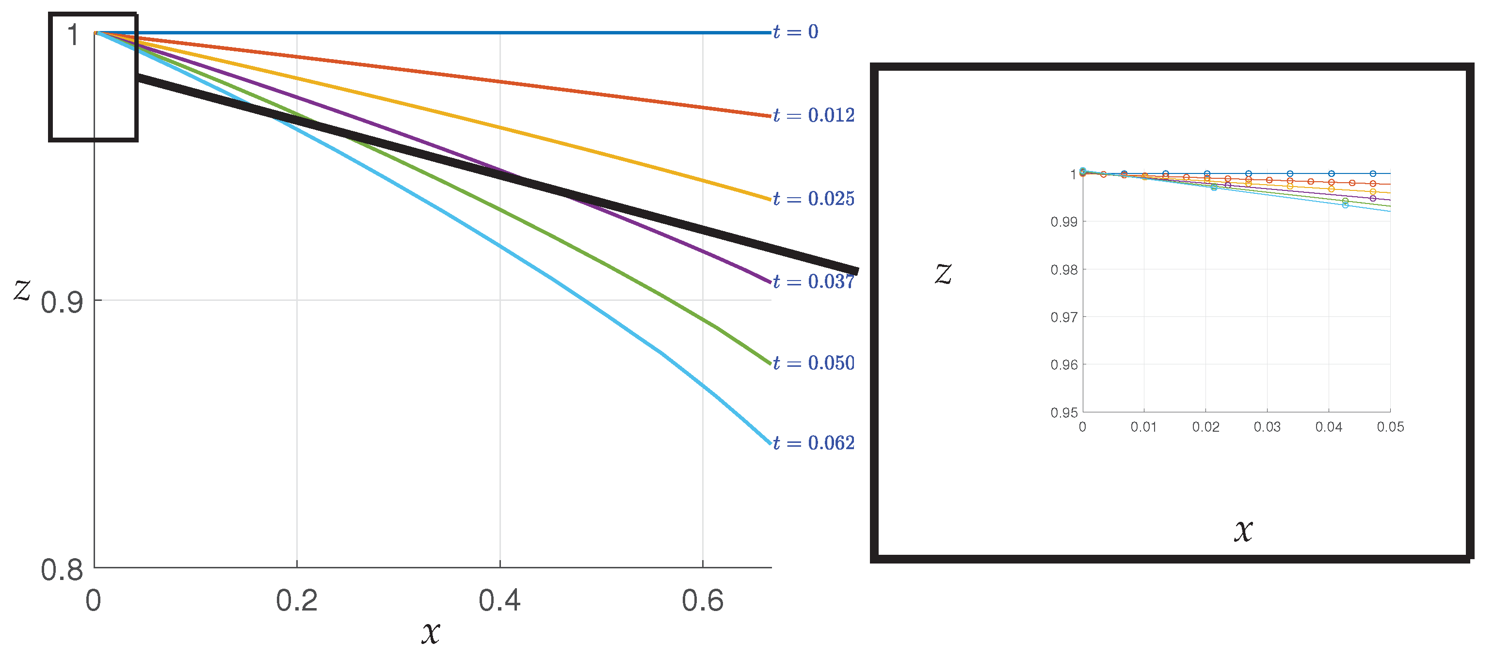
Figure A3.
The new free surface calculation after the convergence errors have been fixed using mesh reduction on the free surface.
Figure A3.
The new free surface calculation after the convergence errors have been fixed using mesh reduction on the free surface.

Convergence of the free surface in this study is dependent on the time steps, . When the time steps are set too high, similar errors to those seen in Figure A2 may occur, but potentially in a different region of the free surface. To obtain a smooth curve and avoid such errors, it is necessary to adjust the value of until convergence is achieved, as demonstrated in Figure A3. It should be noted that altering the time steps will not affect the real-time results of the free surface, as all values of yield the same result at a given moment, as seen in Figure 10, where each value of at both 1 h and 2 h produced identical results.
Appendix B. Calculating the Trapezoidal Dam for Unsteady-State Flow
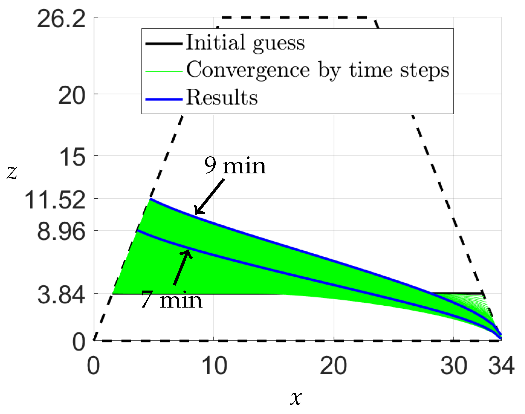
In order to obtain a solution for the unsteady-state flow, an initial guess is required. In this study, for the experiment conducted by Desai et al. [14], a straight line representing the inflow height at 3 min is used as the initial guess, as shown in Figure A4. The boundary conditions for this case are presented in Equation (2), where is held constant at 0.05 cm throughout the calculation. , on the other hand, increases by 1.28 cm/m and is initially set to 3.84 cm.
Initially, the downstream decrease in the free surface was followed by an increase. Our calculated downstream flow results agreed with the experiment, but they were lower than those reported by Zuyang et al. [15]. This discrepancy may be attributed to the constant value of that was held at 0.05 cm throughout our calculations. To accurately model the water flow through the trapezoidal dam, we imposed the requirement that the edges of the free-surface curve fit the shape of the dam, as depicted by the green lines in Figure A4. Additional solutions for this problem are displayed in Figure 13.
Figure A4.
Convergence of the free surface of the unsteady-state flow.

References
- Aksoy, C.O. Chemical injection application at tunnel service shaft to prevent ground settlement induced by groundwater drainage: A case study. Int. J. Rock Mech. Min. Sci. 2008, 45, 376–383. [Google Scholar] [CrossRef]
- Chen, Y.F.; Hong, J.M.; Zheng, H.K.; Li, Y.; Hu, R.; Zhou, C.B. Evaluation of groundwater leakage into a drainage tunnel in Jinping-I arch dam foundation in southwestern China: A case study. Rock Mech. Rock Eng. 2016, 49, 961–979. [Google Scholar] [CrossRef]
- Akai, K.; Ohnishi, Y.; Nishigaki, M. Finite element analysis of saturated-unsaturated seepage in soil. Proc. Jpn. Soc. Civ. Eng. 1977, 1977, 87–96. [Google Scholar] [CrossRef] [PubMed]
- Xia, C.; Lv, Z.; Li, Q.; Huang, J.; Bai, X. Transversely isotropic frost heave of saturated rock under unidirectional freezing condition and induced frost heaving force in cold region tunnels. Cold Reg. Sci. Technol. 2018, 152, 48–58. [Google Scholar] [CrossRef]
- Dai, Y.; Zhou, Z. Steady seepage simulation of underground oil storage caverns based on Signorini type variational inequality formulation. Geosci. J. 2015, 19, 341–355. [Google Scholar] [CrossRef]
- Tsubaki, R.; Kawah, Y.; Ueda, Y. Railway Embankment Failure due to Ballast Layer Breach Caused by Inundation Flows. Nat. Hazards 2017, 87, 717–738. [Google Scholar] [CrossRef]
- Atmojo, P.S.; Sachro, S.S.; Edhisono, S.; Hadihardaja, I.K. Simulation of the Effectiveness of the Scouring Prevention Structure at the External Rail Ballast using Physical Model. Int. J. Geomate 2018, 15, 178–185. [Google Scholar] [CrossRef]
- Polemio, M.; Lollino, P. Failure of infrastructure embankments induced by flooding and seepage: A neglected source of hazard. Nat. Hazards Earth Syst. Sci. 2011, 11, 3383–3396. [Google Scholar] [CrossRef]
- Alrdadi, R.; Meylan, M.H. Modelling Water Flow through Railway Ballast with Random Permeability and a Free Boundary. Appl. Math. Model. 2021, 103, 36–50. [Google Scholar] [CrossRef]
- Isaacs, L.T. Adjustment of Phreatic Line in Seepage Analysis by Finite Element Method; University of Queensland: St Lucia, Australia, 1979. [Google Scholar]
- Ghataora, G.S.; Rushton, K. Movement of water through ballast and subballast for dual-line railway track. Transp. Res. Rec. 2012, 2289, 78–86. [Google Scholar] [CrossRef]
- Chakib, A.; Nachaoui, A. Nonlinear programming approach for a transient free boundary flow problem. Appl. Math. Comput. 2005, 160, 317–328. [Google Scholar] [CrossRef]
- Di Nucci, C. Unsteady free surface flow in porous media: One-dimensional model equations including vertical effects and seepage face. Comptes Rendus Mécanique 2018, 346, 366–383. [Google Scholar] [CrossRef]
- Desai, C.S.; Lightner, J.G.; Somasundaram, S. A numerical procedure for three-dimensional transient free surface seepage. Adv. Water Resour. 1983, 6, 175–181. [Google Scholar] [CrossRef]
- Ye, Z.; Fan, Q.; Huang, S.; Cheng, A. A one-dimensional line element model for transient free surface flow in porous media. Appl. Math. Comput. 2021, 392, 125747. [Google Scholar] [CrossRef]
- Alrdadi, R.; Meylan, M.H. Modelling Experimental Measurements of Fluid Flow through Railway Ballast. Fluids 2022, 7, 118. [Google Scholar] [CrossRef]
- France, P.W.; Parekh, C.; Peters, J.C.; Taylor, C. Numerical analysis of free surface seepage problems. J. Irrig. Drain. Div. 1971, 97, 165–179. [Google Scholar] [CrossRef]
- Mills, K.G. Computation of Post-Drawdown Seepage in Earth Dams by Finite Elements; University of Queensland: St Lucia, Australia, 1970. [Google Scholar]
- Elliott, C.M.; Ockendon, J.R. Weak and Variational Methods for Moving Boundary Problems; Pitman Publishing: Boston, MA, USA, 1982; Volume 59. [Google Scholar]
- Tennakoon, N.; Indraratna, B.; Rujikiatkamjorn, C.; Nimbalkar, S.; Neville, T. The Role of Ballast-Fouling Characteristics on the Drainage Cpacity of Rail Substructure. Geotech. Test. J. 2012, 35, 629–640. [Google Scholar] [CrossRef]
Figure 1.
Schematic diagram of the problem with a free boundary.

Figure 2.
Schematic showing the evolution of the free boundary position with respect to time.

Figure 3.
The free surface elevations for Case 1 of this study and Di Nucci [13].
Figure 3.
The free surface elevations for Case 1 of this study and Di Nucci [13].

Figure 4.
The free surface elevations for Case 1 for Chakib and Nachaou [12].
Figure 4.
The free surface elevations for Case 1 for Chakib and Nachaou [12].

Figure 5.
The converged free surface for Case 1 for the studies listed (Di Nucci [13], Chakib and Nachaou [12], Elliott and Ockendon [19] and Alrdadi and Meylan [9]).

Figure 6.
The free surface elevation at when (Di Nucci [13], Chakib and Nachaou [12], Elliott and Ockendon [19] and Alrdadi and Meylan [9]).

Figure 7.
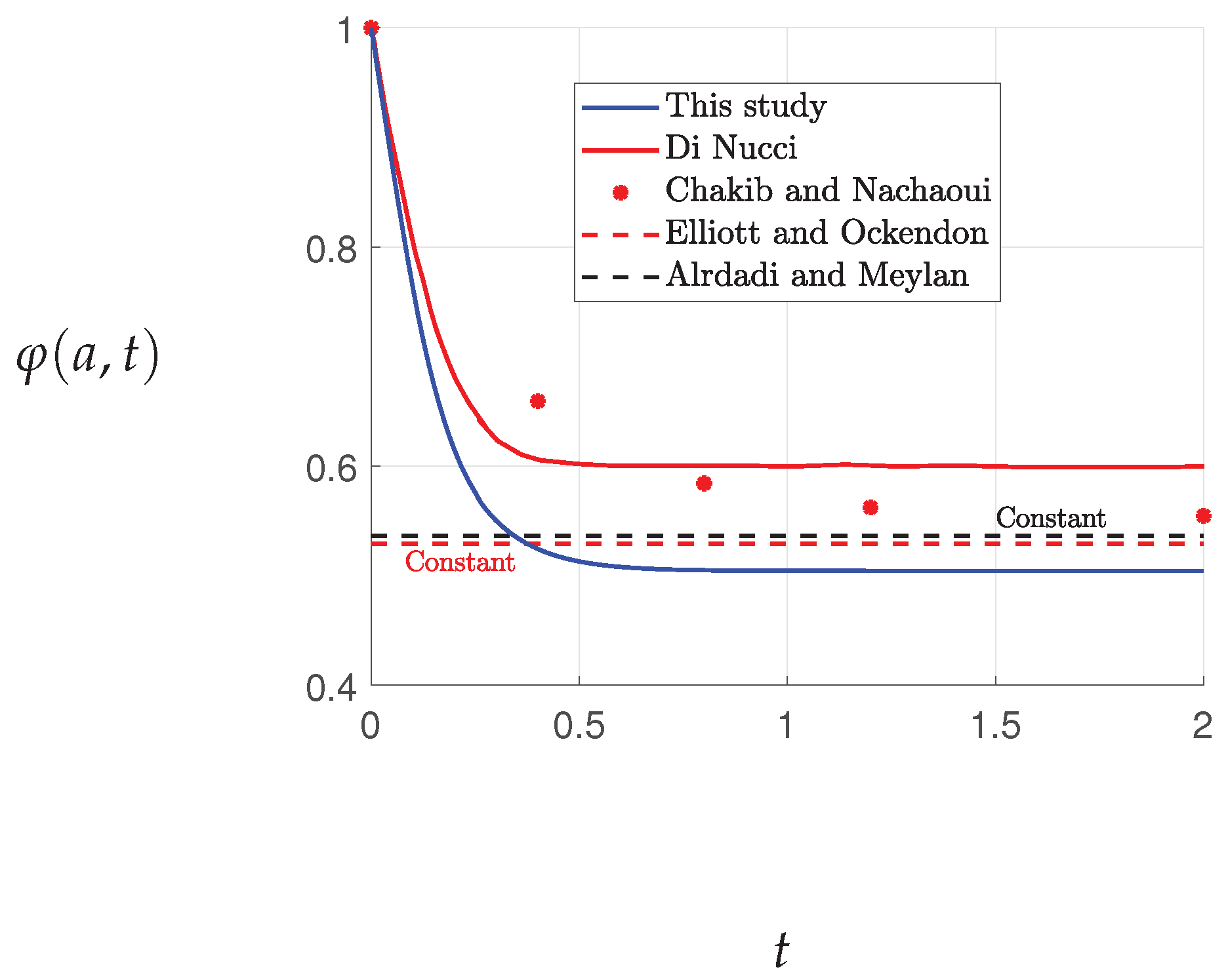
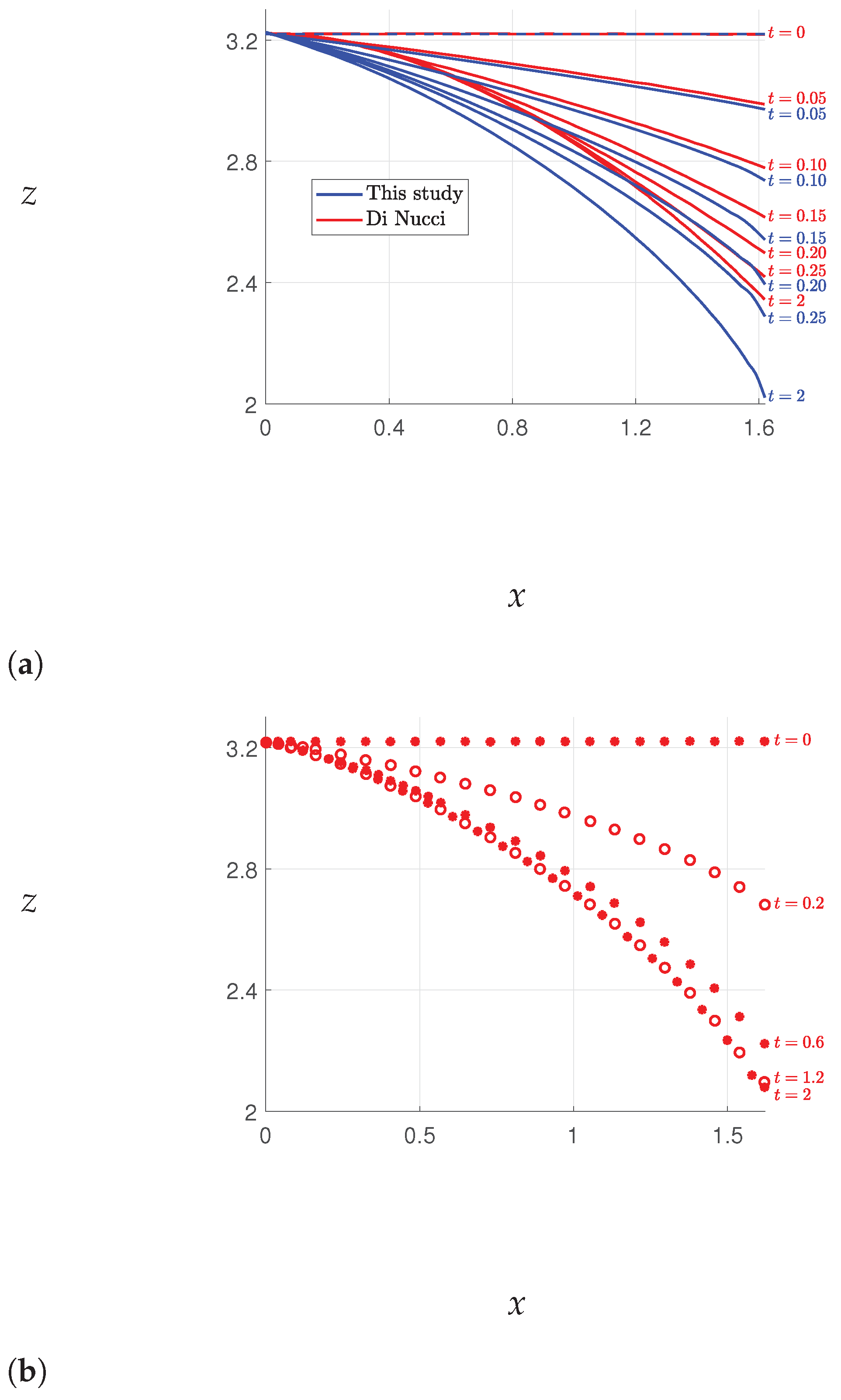
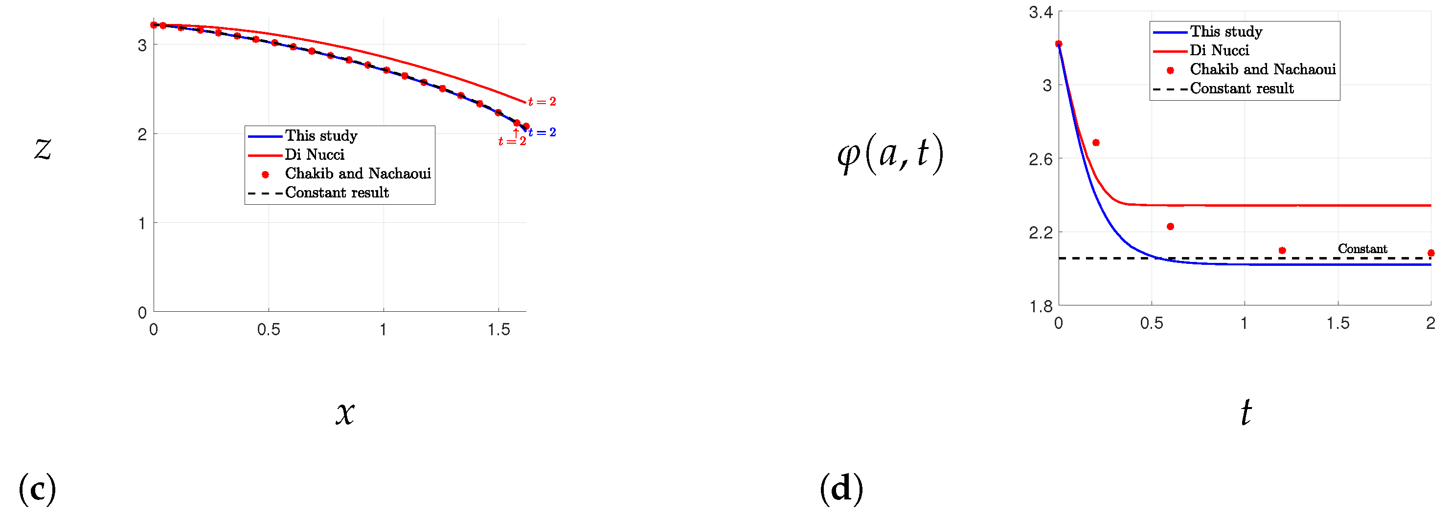
The free surface convergence of Case 2. (a) The free surface elevations of this study and Di Nucci [13]. (b) The free surface elevations of Chakib and Nachaou [12]. (c) The converged free surface for the studies listed. (d) The free surface elevation at when .


Figure 8.
The free surface convergence of Case 3. (a) The free surface elevations of this study and Di Nucci [13]. (b) The free surface elevations of Chakib and Nachaou [12]. (c) The converged free surface for the studies listed. (d) The free surface elevation at when .


Figure 9.
Free-surface positions of the rectangular dam, comparing our results with Ye et al. [15].
Figure 9.
Free-surface positions of the rectangular dam, comparing our results with Ye et al. [15].

Figure 10.
Free surface positions for different values of .

Figure 11.
Schematic diagram of the trapezoidal model.

Figure 12.
The variation in the water level for inflow with respect to time [14].
Figure 12.
The variation in the water level for inflow with respect to time [14].

Figure 13.
Free surface positions of Desai et al.’s experiment [14] and the calculations of Ye et al. [15] compared with our results.

Figure 14.
The railway ballast geometry following the Australian track dimensions [20].
Figure 14.
The railway ballast geometry following the Australian track dimensions [20].

Figure 15.
Models of realistic railway ballast include fouling following the ratio in [20]. The colours correspond to the different fouling ratios shown in Figure 16.

Figure 16.
Fouling ratio or Void Contaminant Index (VCI) and the equivalent hydraulic conductivity : (a) m/s; (b) m/s; (c) m/s; (d) m/s [9].
Figure 16.
Fouling ratio or Void Contaminant Index (VCI) and the equivalent hydraulic conductivity : (a) m/s; (b) m/s; (c) m/s; (d) m/s [9].

Figure 17.
Free surface of steady-state flow with respect to time for different models.

Figure 18.
Sudden upstream flow for Clean ballast and Model 1.


Disclaimer/Publisher’s Note: The statements, opinions and data contained in all publications are solely those of the individual author(s) and contributor(s) and not of MDPI and/or the editor(s). MDPI and/or the editor(s) disclaim responsibility for any injury to people or property resulting from any ideas, methods, instructions or products referred to in the content. |
© 2023 by the authors. Licensee MDPI, Basel, Switzerland. This article is an open access article distributed under the terms and conditions of the Creative Commons Attribution (CC BY) license (https://creativecommons.org/licenses/by/4.0/).
Share and Cite
MDPI and ACS Style
Alrdadi, R.; Meylan, M.H. Modelling Time-Dependent Flow through Railway Ballast. Fluids 2023, 8, 170. https://doi.org/10.3390/fluids8060170
AMA Style
Alrdadi R, Meylan MH. Modelling Time-Dependent Flow through Railway Ballast. Fluids. 2023; 8(6):170. https://doi.org/10.3390/fluids8060170
Chicago/Turabian StyleAlrdadi, Raed, and Michael H. Meylan. 2023. "Modelling Time-Dependent Flow through Railway Ballast" Fluids 8, no. 6: 170. https://doi.org/10.3390/fluids8060170