Vortex Model of Plane Couette Flow

Abstract

We present the theoretical description of plane Couette flow based on the previously proposed equations of vortex fluid, which take into account both the longitudinal flow and the vortex tubes rotation. It is shown that the considered equations have several stationary solutions describing different types of laminar flow. We also discuss the simple model of turbulent flow consisting of vortex tubes, which are moving chaotically and simultaneously rotating with different phases. Using the Boussinesq approximation, we obtain an analytical expression for the stationary profile of mean velocity in turbulent Couette flow, which is in good agreement with experimental data and results of direct numerical simulations. Our model demonstrates that near-wall turbulence can be described by a coordinates-independent coefficient of eddy viscosity. In contrast to the viscosity of the fluid itself, this parameter characterizes the turbulent flow and depends on Reynolds number and roughness of the channel walls. Potentially, the proposed model can be considered as a theoretical basis for the experimental measurement of the eddy viscosity coefficient.

1. Introduction

To describe vortex flows, many authors construct Maxwell-type symmetric equations for the local velocity and vorticity vectors [1,2,3,4,5,6]. In particular, these equations are used for the description of turbulent flows [4] and electron–ion plasma in the framework of a hydrodynamic two-fluid model [7,8,9,10,11,12,13,14,15]. However, in all mentioned papers, the additional equation for vortex motion is obtained by taking the “curl” operator from the Euler equation, hence the resulting equation is not independent. Recently, we have developed an alternative approach based on the droplet model of a liquid, which was first introduced by Helmholtz [16]. In particular, we have obtained a closed system of Maxwell-type equations for vortex flow, taking into account the rotation and twisting of vortex tubes [17]. We applied this approach to derive self-consistent hydrodynamic equations for electron–ion plasma [18] and electron fluids in solids [19].

In the present paper, we apply the proposed equations for the description of the plane Couette flow between two moving plates [20,21]. This is a relatively simple canonical type of a walls-bounded shear flow, which is actively studied both theoretically and experimentally. At present, extensive experimental material has accumulated on studies of laminar and turbulent Couette flows [22,23,24,25,26].

The conventional theoretical description of laminar Couette flow is based on the solution of the Navier–Stokes equation for a viscous fluid. The stationary solution of this equation corresponds to a steady flow with a linear velocity distribution in the channel between the plates [20]. The description of turbulent flow is a more difficult task. The turbulent flow is characterized by unsteady eddy movements with a wide range of spatial scales, which are superimposed on a slowly varying mean flow. Vortices mix fluid and are responsible for the higher rates of momentum, mass, and heat transfer from large to small scales. In accordance with the concept of Reynolds decomposition, in this case, all quantities in a liquid can be represented as a composition of mean and fluctuating values, and the averaged turbulent flow is described by the Reynolds-averaged Navier–Stokes (RANS) equation for mean values [27,28]. The main problem related to this description is finding the Reynolds stress tensor, which takes into account the effect of velocity fluctuations on the average flow characteristics [28]. There are several approaches for calculation of the Reynolds tensor and closing the system of equations [29,30,31,32,33,34,35,36,37,38,39]. Boussinesq proposed the concept of turbulent viscosity [29], establishing a relationship between stress tensor and mean flow velocity. However, in order to obtain a satisfactory match with the experimental data within the framework of the RANS equation, it is commonly assumed that the eddy viscosity coefficient depends on the coordinates in the turbulent flow, which requires the development of complex models of the boundary layer using additional equations [31,32,33,34,35,36,37]. With the development of computer technology, different methods for the direct numerical simulations (DNS) based on the solution of the non-stationary RANS equation have become widespread. These methods allow one to simulate the evolution of unsteady flows and calculate the average values of different physical characteristics [35,36,37,38,39]. In particular, the DNS are in demand in engineering calculations of complex flows. However, the requirement for a fine grid for calculations significantly limits the possibilities of these methods, especially at high Reynolds numbers.

Although the existing analytical models of turbulence provide adequate descriptions of experimental data, they contain many fitting parameters and are difficult to analyze. The advantages and disadvantages of various models are considered in [40,41]. A relatively simple analytical model of the turbulent Couette flow was proposed in [31]. It satisfactorily describes the experimental distributions of mean velocity in the central region of the flow, however, the matching of the velocity profiles near the walls requires additional assumptions related to the properties of the eddy viscosity in this region. Therefore, there is still a need for a simple analytical model suitable for the estimation calculations and simple explanation of experimental results.

In the model proposed in this article, vortex tubes are directly involved in the formation of walls-bounded flow, which is especially important in the case of turbulent motion. The theoretical description of turbulent flow, in addition to the RANS equation, includes an equation describing the motion of vortex tubes. This makes it possible to obtain simple analytical solutions for the profiles of the mean velocity in Couette flow. Our model contains only two fitting parameters, as well as the calculated mean velocity profiles in a good agreement with the experimental data and DNS in the entire cross section of the turbulent flow and for various Reynolds numbers (Re).

2. Model of Vortex Plane Couette Flow

We consider a flow of viscous vortex fluid formed between two infinite, parallel plates moving relative to each other in opposite directions (Figure 1).

As we previously showed in [17], a vortex isentropic flow of viscous fluid is described by the following symmetric system of equations:

$$\begin{array}{l}\frac{1}{c}\left(\frac{\partial }{\partial t}+\left(\overrightarrow{v}\cdot \overrightarrow{\nabla }\right)-\nu \mathsf{\Delta }\right)\overrightarrow{v}+\overrightarrow{\nabla }\times \overrightarrow{w}+\overrightarrow{\nabla }u=0,\\ \frac{1}{c}\left(\frac{\partial }{\partial t}+\left(\overrightarrow{v}\cdot \overrightarrow{\nabla }\right)-\nu \mathsf{\Delta }\right)u+\overrightarrow{\nabla }\cdot \overrightarrow{v}=0,\\ \frac{1}{c}\left(\frac{\partial }{\partial t}+\left(\overrightarrow{v}\cdot \overrightarrow{\nabla }\right)-\nu \mathsf{\Delta }\right)\overrightarrow{w}-\overrightarrow{\nabla }\times \overrightarrow{v}+\overrightarrow{\nabla }\xi =0,\\ \frac{1}{c}\left(\frac{\partial }{\partial t}+\left(\overrightarrow{v}\cdot \overrightarrow{\nabla }\right)-\nu \mathsf{\Delta }\right)\xi +\overrightarrow{\nabla }\cdot \overrightarrow{w}=0.\end{array}$$

(1)

Here, $c$ is a speed of sound, $\overrightarrow{v}$ is a local velocity, $\nu$ is the kinematic viscosity, $\overrightarrow{\nabla }$ is the Hamilton operator, and $\mathsf{\Delta }$ is the Laplace operator. The value $u$ is proportional to the enthalpy.

$$\begin{array}{l}u=\frac{1}{c}\epsilon ,\\ d\epsilon =\frac{c^2}{\rho }d \rho ,\end{array}$$

(2)

where $\epsilon$ is an enthalpy per unit mass and $\rho$ is a fluid density. The vector $\overrightarrow{w}$ characterizes the rotation of the vortex tube around its axis.

$$\begin{array}{l}\overrightarrow{w}=2c \overrightarrow{\theta },\\ \overrightarrow{\omega }=\frac{d\overrightarrow{\theta }}{dt},\end{array}$$

(3)

where $\overrightarrow{\theta }$ is the angular vector of rotation of the vortex tube and $\overrightarrow{\omega }$ is the angular velocity of the vortex tube rotation. The value $\xi$ characterizes the twisting of the vortex tube.

$$|\xi |=c \gamma ,$$

(4)

where $\gamma$ is the twisting angle of the vortex tube [17]. To simplify the model, we assume that the liquid is incompressible ($\rho =const,\hspace{0.33em} u=const$) and neglect the twisting of the vortex tubes ($\xi =0$). Then, the system of equations describing the motion of the fluid takes the following form:

$$\begin{array}{l}\frac{1}{c}\left(\frac{\partial }{\partial t}+\left(\overrightarrow{v}\cdot \overrightarrow{\nabla }\right)-\nu \mathsf{\Delta }\right)\overrightarrow{v}+\overrightarrow{\nabla }\times \overrightarrow{w}=0,\\ \frac{1}{c}\left(\frac{\partial }{\partial t}+\left(\overrightarrow{v}\cdot \overrightarrow{\nabla }\right)-\nu \mathsf{\Delta }\right)\overrightarrow{w}-\overrightarrow{\nabla }\times \overrightarrow{v}=0,\\ \overrightarrow{\nabla }\cdot \overrightarrow{v}=0,\\ \overrightarrow{\nabla }\cdot \overrightarrow{w}=0.\end{array}$$

(5)

In plane flow, we assume that for the one-dimensional motion along the X axis, the velocity $\overrightarrow{v}$ has only an X component and depends only on the Y coordinate $v_x=v_x(y,t)$. Similarly, in plane flow, the vector of rotation angle $\overrightarrow{w}$ has only a Z component and depends only on the Y coordinate $w_z=w_z(y,t)$. Thus, the system of equations for the plane flow of vortex fluid takes the following form:

$$\begin{array}{l}\frac{1}{c}\frac{\partial v_x}{\partial t}-\frac{\nu }{c}\frac{{\partial }^2{v}_x}{\partial y^2}+\frac{\partial w_z}{\partial y}=0,\\ \frac{1}{c}\frac{\partial w_z}{\partial t}-\frac{\nu }{c}\frac{{\partial }^2{w}_z}{\partial y^2}+\frac{\partial v_x}{\partial y}=0.\end{array}$$

(6)

These equations make it possible to describe the plane Couette flow taking into account the effects associated with the rotation of vortex tubes.

3. Laminar Plane Couette Flow of Vortex Fluid

3.1. Stationary Flow without Rotation of Vortex Tubes

First, we consider a stationary flow when the angular velocity of the vortex tubes rotation is equal to zero (${\omega }_z=0$). We assume that the functions $v_x(y)$ and $w_z(y)$ are time independent. Then, the system of Equation (6) takes the following form:

$$\begin{array}{l}-\lambda \frac{{\partial }^2{v}_x}{\partial y^2}+\frac{\partial w_z}{\partial y}=0,\\ -\lambda \frac{{\partial }^2{w}_z}{\partial y^2}+\frac{\partial v_x}{\partial y}=0.\end{array}$$

(7)

Here, we introduce the parameter $\lambda =\nu /c$. In addition, we assume that for the liquid at the plate surfaces, the conditions of complete no-slip are realized. This means that the near-wall liquid layer moves at the same speed as the plate and the vortex tubes are rigidly attached to the wall without the possibility of rotation around their axis. This brings us to the following boundary conditions:

$$\begin{array}{l}{v}_x (h)=\mathrm{v},\\ v_x (-h)=-\mathrm{v},\\ w_z (h)=w_z (-h)=0.\end{array}$$

(8)

The solutions of system (7) satisfying the boundary conditions (8) are

$$v_x=\mathrm{v}\frac{\sinh (y/\lambda )}{\sinh (h/\lambda )},$$

(9)

$$w_z=\mathrm{v}\frac{\cosh (y/\lambda )-\cosh (h/\lambda )}{\sinh (h/\lambda )}.$$

(10)

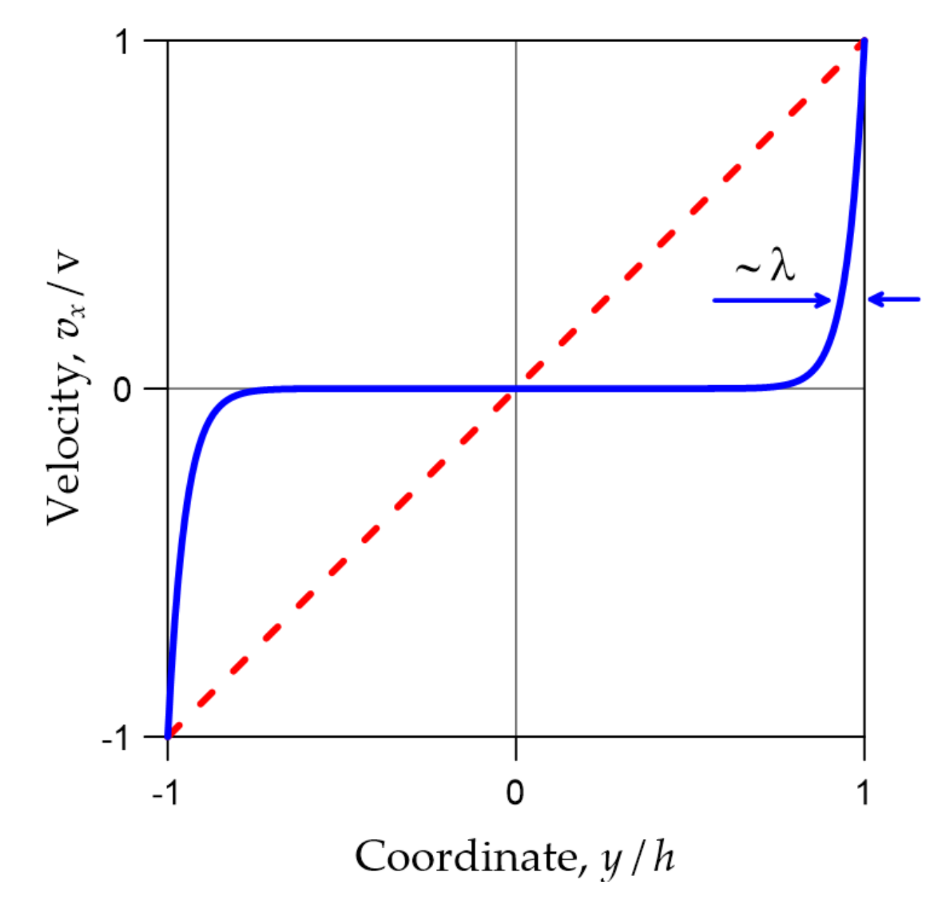
The velocity distribution in the channel between the plates is shown schematically in Figure 2.

Since for the majority of experimentally realized channels (except very thin capillary channels), $h/\lambda \gg 1$, such laminar flow is realized only near the plate’s surface.

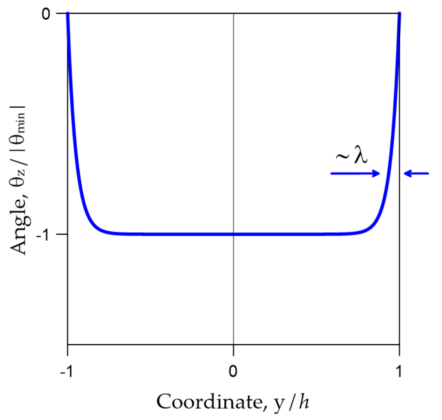
Schematically, the distribution of the angle of the vortex tubes rotation (10) is shown in Figure 3.

According to (9), the vortex of velocity (vorticity, $\overrightarrow{\mathsf{\Omega }}=\overrightarrow{\nabla }\times \overrightarrow{v}$) has only a Z component, which is equal to

$${\mathsf{\Omega }}_z= -\frac{v}{\lambda }\frac{\cosh (y/\lambda )}{\sinh (h/\lambda )}.$$

(11)

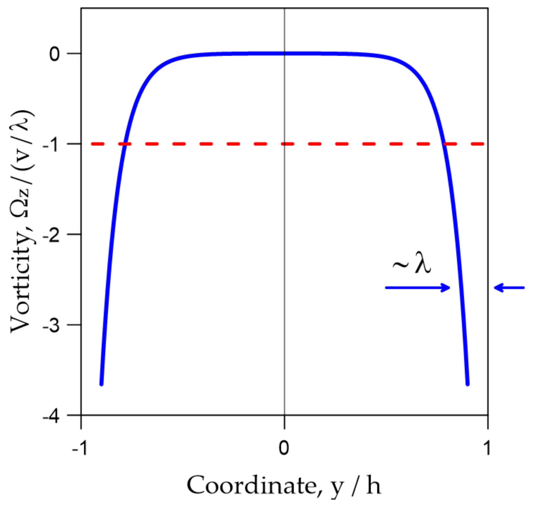
The distribution of the vorticity in the channel between the plates is shown schematically in Figure 4.

3.2. Flow with in-Phase Rotation of Vortex Tubes

Another stationary flow satisfying Equation (6) is characterized by a uniform field of vortex tubes rotating at constant angular velocity ${\omega }_z=const$ and having the same phases. We find a solution for the angle of vortex tubes rotation as

$$w_z(t)= 2c {\omega }_{z}t.$$

(12)

In this case, system (6) takes the following form

$$\begin{array}{l}\frac{{\partial }^2{v}_x}{\partial y^2}=0,\\ 2{\omega }_z+\frac{\partial v_x}{\partial y}=0,\end{array}$$

(13)

with boundary conditions

$$\begin{array}{l}{v}_x(h)=\mathrm{v},\\ v_x(-h)=-\mathrm{v}.\end{array}$$

(14)

From the first equation of system (13), we obtain

$$v_x=\frac{\mathrm{v}}{h}y.$$

(15)

From expression (12), we obtain

$${\theta }_z(t)={\omega }_{z}t.$$

(16)

From the second equation of system (13), we obtain the relationship between the angular velocity of tubes rotation and the velocity of the plates:

$${\omega }_z=-\frac{\mathrm{v}}{2h}.$$

(17)

Expression (17) shows that in this case, the vortex tubes rotate with the maximum angular velocity determined by the speed of the plates. The vorticity is constant over the channel cross section and is equal to

$${\mathsf{\Omega }}_z=-\frac{\mathrm{v}}{h}=2{\omega }_z.$$

(18)

The distributions of velocity (15) and vorticity (18) are shown in Figure 2 and Figure 4 by dotted lines. Stationary distributions (15) and (18) coincide with the known classical solutions for the Couette flow.

3.3. Case of Vortex Tubes Rotating with Different Phases

Let us consider a stationary flow consisting of vortex tubes oriented along the Z axis and rotating with a constant angular velocity ${\omega }_z=const$ but with different phases ${\phi }_z(y)$ depending on the Y coordinate. We will look for a solution in the form

$$w_z(y,t)=2c {\omega }_{z}t+{\phi }_z(y).$$

(19)

In this case, Equation (6) take the following form:

$$\begin{array}{l}-\lambda \frac{{\partial }^2{v}_x}{\partial y^2}+\frac{\partial {\phi }_z}{\partial y}=0,\\ -\lambda \frac{{\partial }^2{\phi }_z}{\partial y^2}+\frac{\partial v_x}{\partial y}+2{\omega }_z=0.\end{array}$$

(20)

In addition, we take the following boundary conditions:

$$\begin{array}{l}{v}_x(h)=\mathrm{v},\\ v_x(-h)=-\mathrm{v},\\ {\phi }_z(h)={\phi }_z(-h)= 0.\end{array}$$

(21)

The solution of system (20) can be represented in the following form:

$$v_x=\alpha v\frac{y}{h}+(1-\alpha ) \mathrm{v}\frac{\sinh (y/\lambda )}{\sinh (h/\lambda )},$$

(22)

$${\phi }_z=(1-\alpha ) \mathrm{v}\frac{\cosh (y/\lambda )-\cosh (h/\lambda )}{\sinh (h/\lambda )},$$

(23)

where the dimensionless parameter $\alpha$ is

$$\alpha =-\frac{2{\omega }_{z}h}{v}.$$

(24)

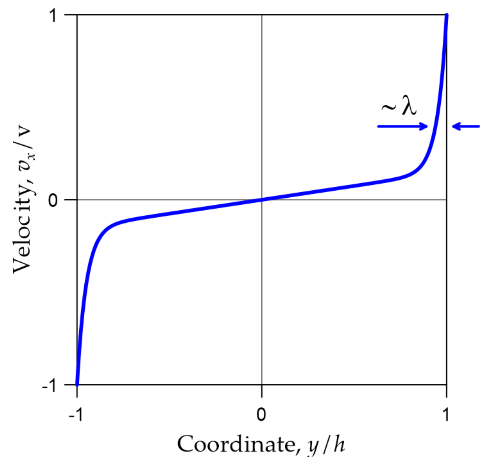
The schematic distribution of velocity over the channel cross section is shown in Figure 5. Note that in the case of $\alpha =0$, the solutions (22)–(24) are reduced to (9)–(10), and in the case of $\alpha =1$, these solutions are reduced to (15)–(17).

4. Turbulent Plane Couette Flow

To describe a turbulent flow, we introduce the time-averaged values of the flow velocities, denoting them as ${\overline{v}}_x,\hspace{0.33em}{\overline{v}}_y,\hspace{0.33em}{\overline{v}}_z$, and corresponding fluctuations, ${v^{\prime }}_x,\hspace{0.33em}{v^{\prime }}_y,\hspace{0.33em}{v^{\prime }}_z$. Then, the local velocities of the turbulent flow are written in the following form:

$$\begin{array}{l}{v}_x={\overline{v}}_x+{v^{\prime }}_x,\\ v_y={\overline{v}}_y+{v^{\prime }}_y,\\ v_z={\overline{v}}_z+{v^{\prime }}_z.\end{array}$$

(25)

Similarly, for the vector of rotation $\overrightarrow{w}$, we have

$$\begin{array}{l}{w}_x={\overline{w}}_x+{w^{\prime }}_x,\\ w_y={\overline{w}}_y+{w^{\prime }}_y,\\ w_z={\overline{w}}_z+{w^{\prime }}_z.\end{array}$$

(26)

Let us consider a plane turbulent flow along the X axis. We take into account that ${\overline{v}}_y=0,\hspace{0.33em}{\overline{v}}_z=0$ and the mean velocity ${\overline{v}}_x(y,t)$ depends only on the Y coordinate. In addition, we assume that vortex tubes are oriented along the Z axis ${\overline{w}}_x=0$, ${\overline{w}}_y=0$, ${\overline{w}}_z={\overline{w}}_z(y,t)$. Substituting (25) and (26) into Equation (6), we account that fluctuations ${v^{\prime }}_x$, ${v^{\prime }}_y$, ${v^{\prime }}_y$ and ${w^{\prime }}_x$, ${w^{\prime }}_y$, ${w^{\prime }}_z$ depend only on the Y coordinate. Then, averaging over time (Reynolds averaging), we obtain:

$$\begin{array}{l}\frac{1}{c}\frac{\partial {\overline{v}}_x}{\partial t}-\frac{\nu }{c}\frac{{\partial }^2{\overline{v}}_x}{\partial y^2}+\frac{1}{c}\frac{\partial }{\partial y}\overline{{v^{\prime }}_x{v^{\prime }}_y}+\frac{\partial {\overline{w}}_z}{\partial y}=0,\\ \frac{1}{c}\frac{\partial {\overline{w}}_z}{\partial t}-\frac{\nu }{c}\frac{{\partial }^2{\overline{w}}_z}{\partial y^2}+\frac{1}{c}\frac{\partial }{\partial y}\overline{{w^{\prime }}_z{v^{\prime }}_y}+\frac{\partial {\overline{v}}_x}{\partial y}=0.\end{array}$$

(27)

Here, $\overline{{v^{\prime }}_x{v^{\prime }}_y}$ and $\overline{{w^{\prime }}_z{v^{\prime }}_y{}_y}$ are the components of the corresponding Reynolds tensors [27,28]. In the framework of Boussinesq approximation [29,30], we can write

$$-\overline{{v^{\prime }}_x{v^{\prime }}_y}={\nu }_T\frac{\partial {\overline{v}}_x}{\partial y},$$

(28)

$$-\overline{{w^{\prime }}_z{v^{\prime }}_y}={\nu }_T\frac{\partial {\overline{w}}_z}{\partial y},$$

(29)

where ${\nu }_T$ is the turbulent (eddy) kinematic viscosity. Let us assume ${\nu }_T=const$, then Equation (27) take the form

$$\begin{array}{l}\frac{1}{c}\frac{\partial {\overline{v}}_x}{\partial t}-\frac{\nu +{\nu }_T}{c}\frac{{\partial }^2{\overline{v}}_x}{\partial y^2}+\frac{\partial {\overline{w}}_z}{\partial y}=0,\\ \frac{1}{c}\frac{\partial {\overline{w}}_z}{\partial t}-\frac{\nu +{\nu }_T}{c}\frac{{\partial }^2{\overline{w}}_z}{\partial y^2}+\frac{\partial {\overline{v}}_x}{\partial y}=0.\end{array}$$

(30)

Let us consider a fully developed stationary flow ${\overline{v}}_x={\overline{v}}_x(y)$, in which the vortex tubes on average rotate with a constant angular velocity ${\overline{\omega }}_z=const$ but with different phases ${\overline{\phi }}_z(y)$. Therefore, we will look for a solution in the following form:

$$\begin{array}{l}{\overline{v}}_x={\overline{v}}_x(y),\\ {\overline{w}}_z(y,t)=2c {\overline{\omega }}_{z}t+{\overline{\phi }}_z(y).\end{array}$$

(31)

Then, Equation (30) take the final form

$$\begin{array}{l}-{\lambda }_T\frac{{\partial }^2{\overline{v}}_x}{\partial y^2}+\frac{\partial {\overline{\phi }}_z}{\partial y}=0,\\ -{\lambda }_T\frac{{\partial }^2{\overline{\phi }}_z}{\partial y^2}+\frac{\partial {\overline{v}}_x}{\partial y}+2{\overline{\omega }}_z=0.\end{array}$$

(32)

Here, we introduced a characteristic scale of the turbulent length ${\lambda }_T=(\nu +{\nu }_T)/c$. As the boundary conditions, we choose

$$\begin{array}{l}{\overline{v}}_x (h)=\mathrm{v},\\ {\overline{v}}_x (-h)=-\mathrm{v},\\ {\overline{\phi }}_z (h)={\overline{\phi }}_z (-h)=0.\end{array}$$

(33)

Then, the solutions of Equation (32) are written as

$${\overline{\mathrm{v}}}_x=\alpha \mathrm{v}\frac{y}{h}+(1-\alpha ) \mathrm{v}\frac{\sinh (y/{\lambda }_{\mathrm{T}})}{\sinh (h/{\lambda }_{\mathrm{T}})},$$

(34)

$${\overline{\phi }}_z=(1-\alpha ) \mathrm{v}\frac{\cosh (y/{\lambda }_{\mathrm{T}})-\cosh (h/{\lambda }_{\mathrm{T}})}{\sinh (h/{\lambda }_{\mathrm{T}})},$$

(35)

$$\alpha =-\frac{2{\overline{\omega }}_{z}h}{\mathrm{v}}.$$

(36)

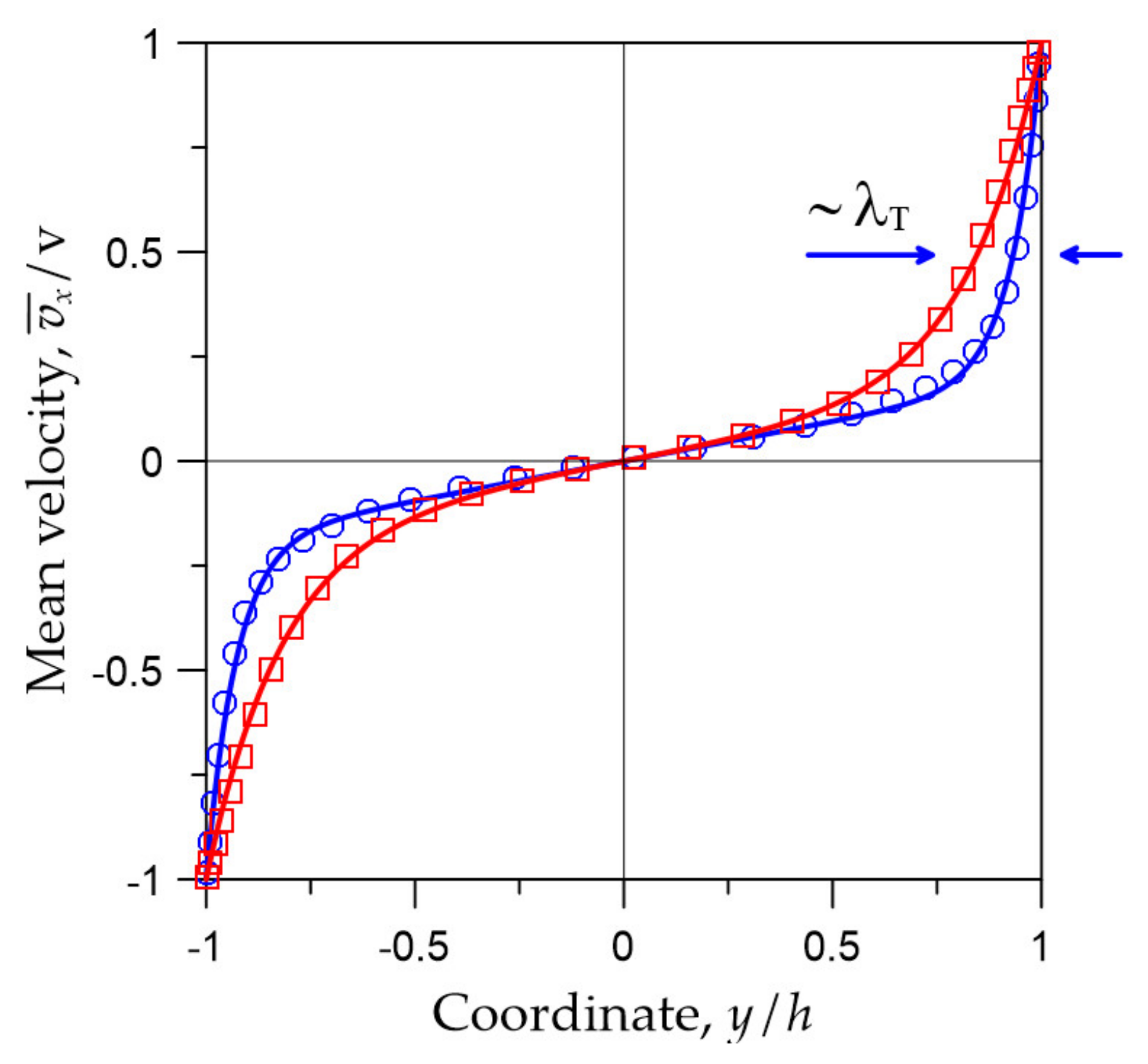
In form, the solutions (34)–(36) coincide with (22)–(24), but they have a different characteristic spatial scale ${\lambda }_{\mathrm{T}}\gg \lambda$, defined by eddy viscosity. As an example, in Figure 6, we demonstrate the comparison of solution (34) with the DNS results for Couette flow with Re = 3000 [42] and Re = 12800 [43].

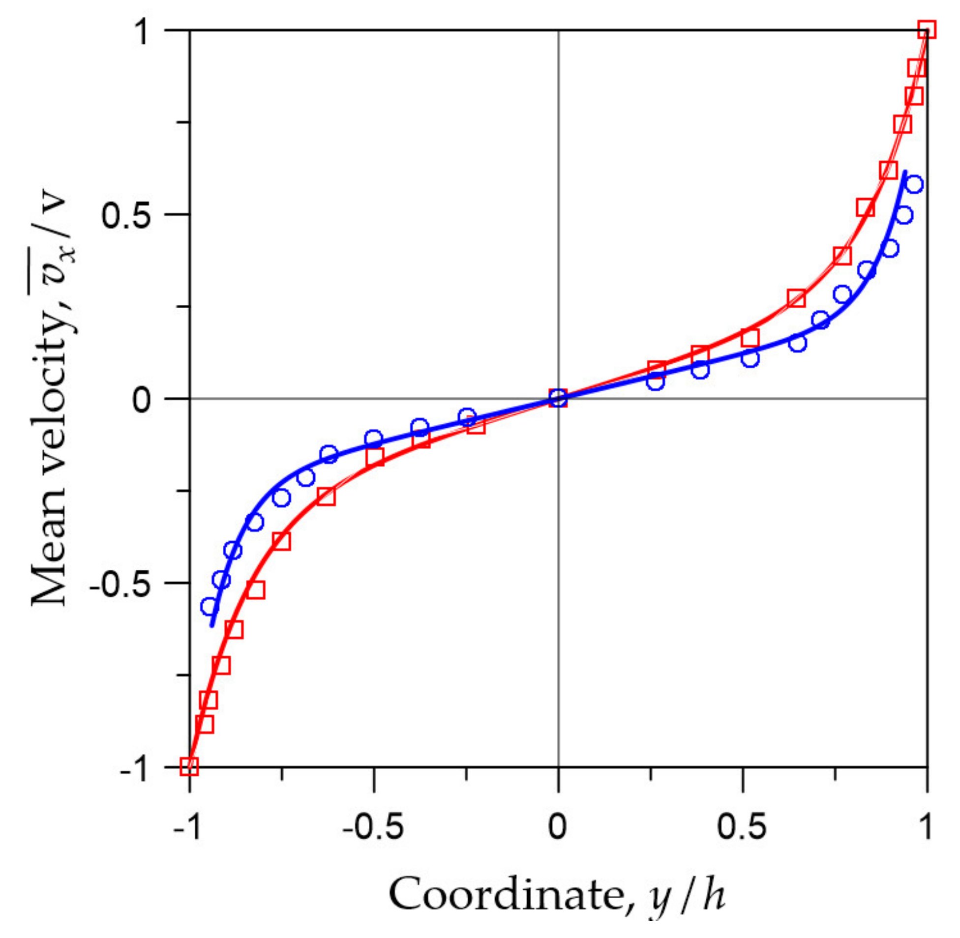
In Figure 7, we show the comparison of mean velocity distribution (34) with experimental results for Re 2900 and 18,000 [44]. In Figure 8, we represent the results of velocity profiles fitting for the flows in channels with smooth and rough walls at close Re [24]. As can be seen, the velocity profiles calculated within the framework of the proposed model are in good agreement with the experimental data and the results of the DNS. We believe that it is possible to reproduce the mean velocity profile for the Couette flow with any Reynolds number by choosing corresponding combinations of the parameters λ_T and α.

5. Discussion

The considered model predicts several types of stationary laminar Couette flow. As can be seen from solutions (9)–(10), the laminar motion without vortex tubes rotation is realized only in a narrow region near the plates. This regime can be important in tribology at low Re, in case of supersmooth plates sliding relative to each other, when a narrow gap between them is filled with a viscous lubricant. However, in the case of macroscopic channels, the plates have rough surfaces and the microvortices in the near-wall region can destroy this flow regime [45,46]. The linear distribution of velocity is obtained in the case when the vortex tubes rotate in-phase with the same angular velocity. On the other hand, taking into account the non-uniform phases of the tubes rotation, we obtained solutions (22)–(24), which describe the combination of the previous two flows.

The proposed model of a vortex fluid allowed us to describe the stationary profile of the mean velocity in turbulent Couette flow. For this purpose, we used the Boussinesq approximation for the Reynolds shear stress tensor. In this simple case, we have obtained a closed system of equations for the time-averaged values ${\overline{v}}_x$ and ${\overline{w}}_z$, which correctly describes turbulent flow. In particular, we have shown that by optimizing the parameters λ_T and $\alpha$ in (34), it is possible to describe both experimental and DNS-produced profiles of mean velocity for turbulent Couette flow.

The experimental data and the results of the DNS (Figure 6 and Figure 7) show that an increase in Re leads to a decrease in the slope of the velocity profile in the central region of the channel and a faster decay in the near-wall region. In the proposed model, the scale of the profile change in the near-wall region is unambiguously determined by the parameter λ_T, which is proportional to the eddy viscosity coefficient (see Figure 6 and Figure 7). The parameter $\alpha$ (which is determined by the speed of walls $\mathrm{v}$ and the velocity of the vortex tubes rotation ${\overline{\omega }}_z$) mainly adjusts the slope of the profile in the central region of the channel. Thus, an important achievement of this model is that, within the framework of the equations for a vortex fluid, the developed turbulence in the near-wall region is described by a constant eddy viscosity coefficient that essentially simplifies the transition layer model. In addition, the comparisons of calculated velocity profiles and experimental data for the Couette flows in channels with smooth and rough walls (Figure 8) show that the shape of the velocity profile for rough wall channels remains the same, only the slope and the rate of near-wall decay are changed. This shows that the model with constant eddy viscosity also works in the case of channels with rough walls. An increase in wall roughness is simply described by an increase in the eddy viscosity coefficient.

Therefore, we emphasize that within the framework of the proposed model, the constant coefficient of eddy viscosity unambiguously characterizes the turbulent motion of the fluid and is determined by the maximum flow velocity (Reynolds number) and the boundary conditions (surface roughness) on the channel walls.

6. Conclusions

Thus, we considered various types of steady state flow in the channel between two plates moving relative to each other based on the equations describing the vortex motion of viscous fluid. We obtained several solutions corresponding to different stationary laminar flows.

It is especially important that the considered model of a vortex fluid made it possible to describe the turbulent Couette flow in the Boussinesq approximation. The calculated average velocity profiles are in good agreement with the experimental data and the results of the DNS. This shows that within the framework of these equations, near-wall turbulence is described by a constant coefficient of eddy viscosity. This model allows a fairly simple interpretation of the average velocity profiles and simple estimates of the eddy viscosity coefficient based on experimental measurements.

In the future, the model of vortex viscous fluid is planned to be applied to describe the plane Poiseuille flow and mixed Poiseuille–Couette flow.

References

- Kambe, T. A new formulation of equation of compressible fluids by analogy with Maxwell’s equations. Fluid Dyn. Res. 2010, 42, 055502. [Google Scholar] [CrossRef]
- Thompson, R.J.; Moeller, T.M. Numerical and closed-form solutions for the Maxwell equations of incompressible flow. Phys. Fluids 2018, 30, 083606. [Google Scholar] [CrossRef]
- Mendes, C.R.; Takakura, F.I.; Abreu, E.M.C.; Neto, J.A.; Silva, P.P.; Frossad, J.V. Helicity and vortex generation. Ann. Phys. 2018, 398, 146–158. [Google Scholar] [CrossRef]
- Marmanis, H. Analogy between the Navier-Stokes equations and Maxwell’s equations: Application to turbulence. Phys. Fluids 1998, 10, 1428–1437. [Google Scholar] [CrossRef]
- Demir, S.; Tanişli, M. Spacetime algebra for the reformulation of fluid field equations. Int. J. Geom. Methods Mod. Phys. 2017, 14, 1750075. [Google Scholar] [CrossRef]
- Tanişli, M.; Demir, S.; Sahin, N. Octonic formulations of Maxwell type fluid equations. J. Math. Phys. 2015, 56, 091701. [Google Scholar] [CrossRef]
- Demir, S.; Uymaz, A.; Tanışlı, M. A new model for the reformulation of compressible fluid equations. Chin. J. Phys. 2017, 55, 115–126. [Google Scholar] [CrossRef]
- Thompson, R.J.; Moeller, T.M. A Maxwell formulation for the equations of a plasma. Phys. Plasmas 2012, 19, 010702. [Google Scholar] [CrossRef]
- Thompson, R.J.; Moeller, T.M. Classical field isomorphisms in two-fluid plasmas. Phys. Plasmas 2012, 19, 082116. [Google Scholar] [CrossRef]
- Jamil, M.; Ahmed, A. New traveling wave solutions of MHD micropolar fluid in porous medium. J. Egypt Math. Soc. 2020, 28, 23. [Google Scholar] [CrossRef]
- Eshraghi, H.; Gibbon, J.D. Quaternions and ideal flows. J. Phys. A Math. Theor. 2008, 41, 344004. [Google Scholar] [CrossRef]
- Demir, S.; Tanişli, M.; Sahin, N.; Kansu, M.E. Biquaternionic reformulation of multifluid plasma equations. Chin. J. Phys. 2017, 55, 1329. [Google Scholar] [CrossRef]
- Demir, S.; Zeren, E. Multifluid plasma equations in terms of hyperbolic octonions. Int. J. Geom. Methods Mod. Phys. 2018, 15, 1850053. [Google Scholar] [CrossRef]
- Chanyal, B.C.; Pathak, M. Quaternionic approach to dual magneto-hydrodynamics of dyonic cold plasma. Adv. High Ener. Phys. 2018, 13, 7843730. [Google Scholar]
- Chanyal, B.C. Quaternionic approach on the Dirac–Maxwell, Bernoulli and Navier– Stokes equations for dyonic fluid plasma. Int. J. Mod. Phys. A 2019, 34, 1950202. [Google Scholar] [CrossRef]
- Helmholtz, H. Über Integrale der hydrodynamischen Gleichungen, welche den Wirbelbewegungen entsprechen. J. Die Reine Angew. Math. 1858, 55, 25–55. [Google Scholar]
- Mironov, V.L.; Mironov, S.V. Generalized sedeonic equations of hydrodynamics. Eur. Phys. J. Plus 2020, 135, 708. [Google Scholar] [CrossRef]
- Mironov, V.L. Self-consistent hydrodynamic two-fluid model of vortex plasma. Phys. Fluids 2021, 33, 037116. [Google Scholar] [CrossRef]
- Mironov, V.L. Self-consistent hydrodynamic model of electron vortex fluid in solids. Fluids 2022, 7, 330. [Google Scholar] [CrossRef]
- Kochin, N.K.; Kibel, I.A.; Roze, N.V. Theoretical Hydrodynamics; John Wiley & Sons: New York, NY, USA, 1964. [Google Scholar]
- Batchelor, G.K. An Introduction to Fluid Dynamics; Cambridge University Press: Cambridge, UK, 1970. [Google Scholar]
- Tillmark, N.; Alfredsson, P.H. Experiments on transition in plane Couette flow. J. Fluid Mech. 1992, 235, 89–102. [Google Scholar] [CrossRef]
- Bech, K.H.; Tillmark, N.; Alfredsson, P.H.; Andersson, H.I. An investigation of turbulent plane Couette flow at low Reynolds numbers. J. Fluid Mech. 1995, 286, 291–325. [Google Scholar] [CrossRef]
- Aydin, E.M.; Leuthersser, H.J. Plane-Couette flow between smooth and rough walls. Experim. Fluids 1991, 11, 302–312. [Google Scholar] [CrossRef]
- Bottin, S.; Chate, H. Statistical analysis of the transition to turbulence in plane Couette flow. Eur. Phys. J. B 1998, 6, 143–155. [Google Scholar] [CrossRef]
- Kitoh, O.; Nakabyashi, K.; Nishimura, F. Experimental study on mean velocity and turbulence characteristics of plane Couette flow: Low-Reynolds-number effects and large longitudinal vortical structure. J. Fluid Mech. 2005, 539, 199–227. [Google Scholar] [CrossRef]
- Reynolds, O. On the dynamical theory of incompressible viscous fluids and the determination of the criterion. Phil. Trans. Royal Soc. London A 1895, 186, 123–164. [Google Scholar]
- McComb, W.D. Theory of turbulence. Rep. Prog. Phys. 1995, 58, 1117–1206. [Google Scholar] [CrossRef]
- Boussinesq, J. Essai sur la Theorie des Eaux Courantes. Memoires Presentes par Divers Savants a l’Academie des Sciences de l’Institut National de France; Tome XXIII, No 1.; Imprimerie Nationale: Paris, France, 1877. [Google Scholar]
- Schmitt, F.G. About Boussinesq’s turbulent viscosity hypothesis: Historical remarks and a direct evaluation of its validity. Comptes Rendus Méc. 2007, 335, 617–627. [Google Scholar] [CrossRef]
- Henry, F.S.; Reynolds, A.J. Analytical solution of two gradient-diffusion models applied to turbulent Couette flow. ASME J. Fluids Eng. 1984, 106, 211–216. [Google Scholar] [CrossRef]
- Nimura, T.; Tsukahara, T. Viscoelasticity-induced instability in plane Couette flow at very low Reynolds number. Fluids 2022, 7, 241. [Google Scholar] [CrossRef]
- Ribau, A.M.; Ferrás, L.L.; Morgado, M.L.; Rebelo, M.; Afonso, A.M. Semi-analytical solutions for the Poiseuille–Couette flow of a generalised Phan-Thien-Tanner fluid. Fluids 2019, 4, 129. [Google Scholar] [CrossRef]
- Baranovskii, E.S.; Burmasheva, N.V.; Prosviryakov, E.Y. Exact solutions to the Navier–Stokes equations with couple stresses. Symmetry 2021, 13, 1355. [Google Scholar] [CrossRef]
- Andersson, H.I.; Pettersson, B.A. Modeling plane turbulent Couette flow. Int. J. Heat Fluid Flow 1994, 15, 447–455. [Google Scholar] [CrossRef]
- Abe, H.; Kawamura, H.; Matsuo, Y. Direct numerical simulation of a fully developed turbulent channel flow with respect to the Reynolds number dependence. ASME J. Fluids Eng. 2001, 123, 382–393. [Google Scholar] [CrossRef]
- Pirozzoli, S.; Bernardini, M.; Orlandi, P. Turbulence statistics in Couette flow at high Reynolds number. J. Fluid Mech. 2014, 758, 327–343. [Google Scholar] [CrossRef]
- Tsukahara, T.; Kawamura, H.; Shingai, K. DNS of turbulent Couette flow with emphasis on the large-scale structure in the core region. J. Turbul. 2006, 7, N19. [Google Scholar] [CrossRef]
- Sherikar, A.; Disimile, P.J. Parametric study of turbulent Couette flow over wavy surfaces using RANS simulation: Effects of aspect-ratio, wave-slope and Reynolds number. Fluids 2020, 5, 138. [Google Scholar] [CrossRef]
- Sarkar, A.; So, R.M.C. A critical evaluation of near-wall two-equation models against direct numerical simulation data. Int. J. Heat Fluid Flow 1997, 18, 197–208. [Google Scholar] [CrossRef]
- Gerodimos, G.; So, R.M.C. Near-wall modeling of plane turbulent wall jets. ASME J. Fluids Eng. 1997, 119, 304–313. [Google Scholar] [CrossRef]
- Tsukahara, T.; Kawamura, H.; Shingai, K. DNS Database of Wall Turbulence and Heat Transfer, Cou3000_A.dat. Available online: https://www.rs.tus.ac.jp/t2lab/db/cou/cou.html#cou3000 (accessed on 4 April 2023).
- Kawamura, H.; Shingai, K.; Matsuo, Y. DNS Database of Wall Turbulence and Heat Transfer, Cou12800_A.dat. Available online: https://www.rs.tus.ac.jp/t2lab/db/cou/cou.html#cou3000 (accessed on 4 April 2023).
- Reichardt, H. Über die Geschwindigkeitsverteilung in einer geradigen turbulenten Couetteströmung. Z. Angew. Math. Mech. 1956, 36, 26–29. [Google Scholar] [CrossRef]
- Stanislas, M.; Perret, L.; Foucaut, J.M. Vortical structures in the turbulent boundary layer: A possible route to a universal representation. J. Fluid Mech. 2008, 602, 327–382. [Google Scholar] [CrossRef]
- Wang, C.; Gao, Q.; Wang, J.; Wang, B.; Pan, C. Experimental study on dominant vortex structures in near-wall region of turbulent boundary layer based on tomographic particle image velocimetry. J. Fluid Mech. 2019, 874, 426–454. [Google Scholar] [CrossRef]
Figure 1.
Sketch of a system consisting of fluid placed between two infinite plates, which move along the X axis with speed v in opposite directions.
Figure 2.
The steady profiles of flow velocity in the channel between two moving plates. The solid blue line corresponds to the distribution (9). The dotted red line corresponds to the distribution (15).
Figure 3.
Schematic normalized distribution (10) of the angle of the vortex tubes rotation () across the channel .
Figure 4.
Distributions of vorticity in the channel between two moving plates. The solid blue line corresponds to the distribution (11). The dotted red line corresponds to the normalized distribution (18).
Figure 5.
The profile of the fluid velocity in the channel between two moving plates corresponding to the distribution (22).
Figure 6.
Distributions of the mean velocity in a turbulent Couette flow between two moving plates. Squares () are the results of DNS with Re = 3000 [42]; the solid red line corresponds to (34) at λT/h = 0.18, α = 0.165. Circles () are the DNS results with Re = 12800 [43]; the solid blue line corresponds to (34) at λT/h = 0.072, α = 0.189. The characteristic scale of the velocity profiles is .
Figure 7.
Distributions of the mean velocity in a turbulent Couette flow. Squares () are the experimental results for Re = 2900 [44]; the solid red line corresponds to (34) at λT/h = 0.16, α = 0.3. Circles () are the experimental results for Re = 18,000 [44]; the solid blue line corresponds to (34) at λT/h = 0.09, α = 0.24.
Figure 8.
Profiles of the mean velocity in a turbulent Couette flow. Squares () are the experimental data for rough wall channels, Re = 10,850 [24]; the solid red line corresponds to (34) at λT/h = 0.14, α = 0.34. Circles () are the experimental results for smooth wall channels, Re = 9524 [24]; the solid blue line corresponds to (34) at λT/h = 0.065, α = 0.21.
Disclaimer/Publisher’s Note: The statements, opinions and data contained in all publications are solely those of the individual author(s) and contributor(s) and not of MDPI and/or the editor(s). MDPI and/or the editor(s) disclaim responsibility for any injury to people or property resulting from any ideas, methods, instructions or products referred to in the content. |
© 2023 by the authors. Licensee MDPI, Basel, Switzerland. This article is an open access article distributed under the terms and conditions of the Creative Commons Attribution (CC BY) license (https://creativecommons.org/licenses/by/4.0/).
Share and Cite
MDPI and ACS Style
Mironov, V.L.; Mironov, S.V. Vortex Model of Plane Couette Flow. Fluids 2023, 8, 165. https://doi.org/10.3390/fluids8060165
AMA Style
Mironov VL, Mironov SV. Vortex Model of Plane Couette Flow. Fluids. 2023; 8(6):165. https://doi.org/10.3390/fluids8060165
Chicago/Turabian StyleMironov, Victor L., and Sergey V. Mironov. 2023. "Vortex Model of Plane Couette Flow" Fluids 8, no. 6: 165. https://doi.org/10.3390/fluids8060165