
Effect of Horizontal Quasi-Periodic Oscillation on the Interfacial Instability of Two Superimposed Viscous Fluid Layers in a Vertical Hele-Shaw Cell
 , , ,
, , , 
Abstract
:1. Introduction
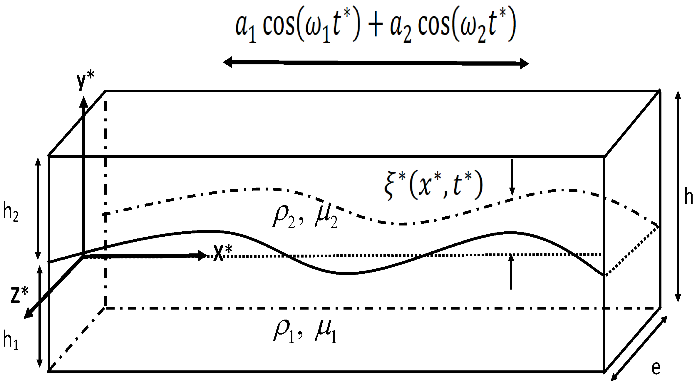
2. Formulation
2.1. Governing Equations
2.2. Base Flows
2.3. Linear Stability
3. Numerical Procedure
4. Results and Discussion
4.1. Validation of the Numerical Procedure
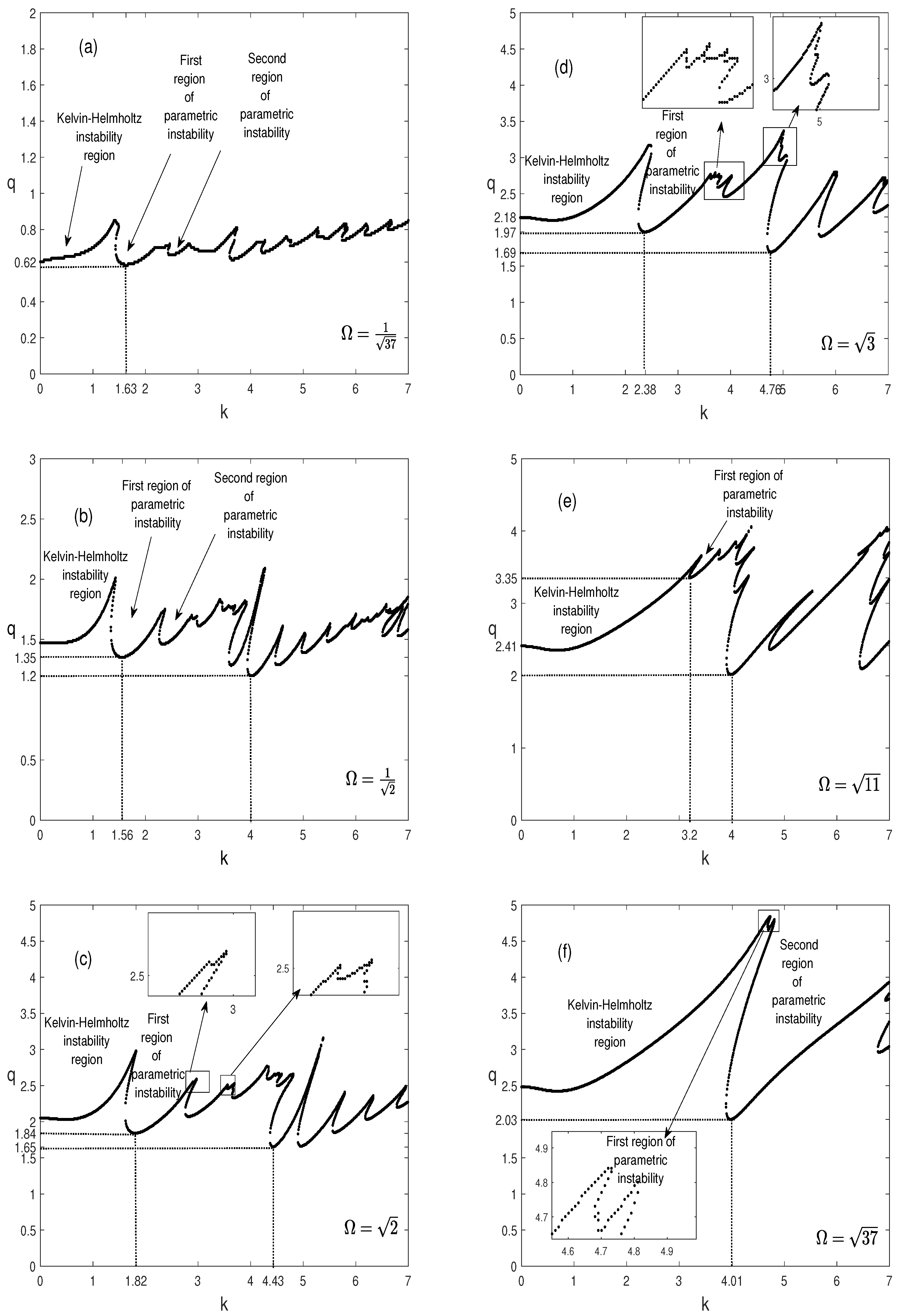
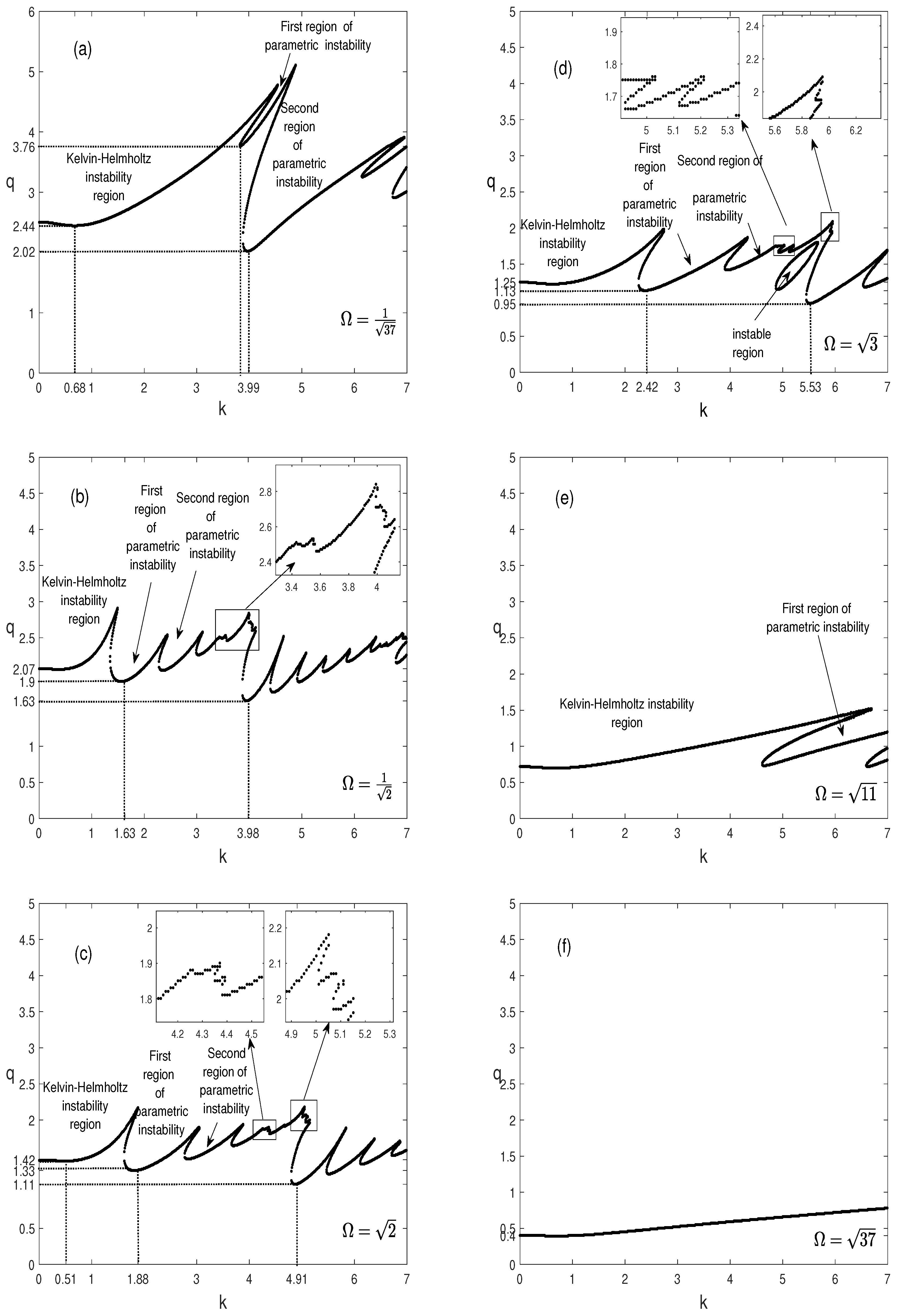
4.2. Effect of the Irrational Frequency Ratio in the Case of Equal Amplitudes of Superimposed Accelerations:
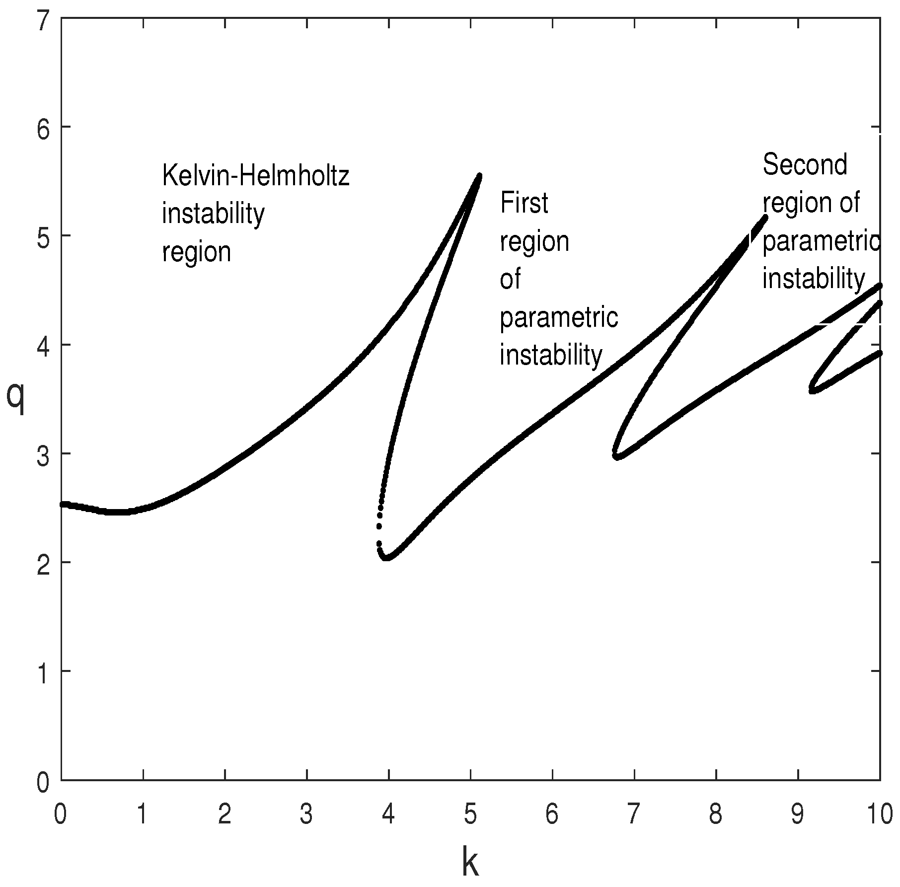
4.2.1. Kelvin-Helmholtz Instability
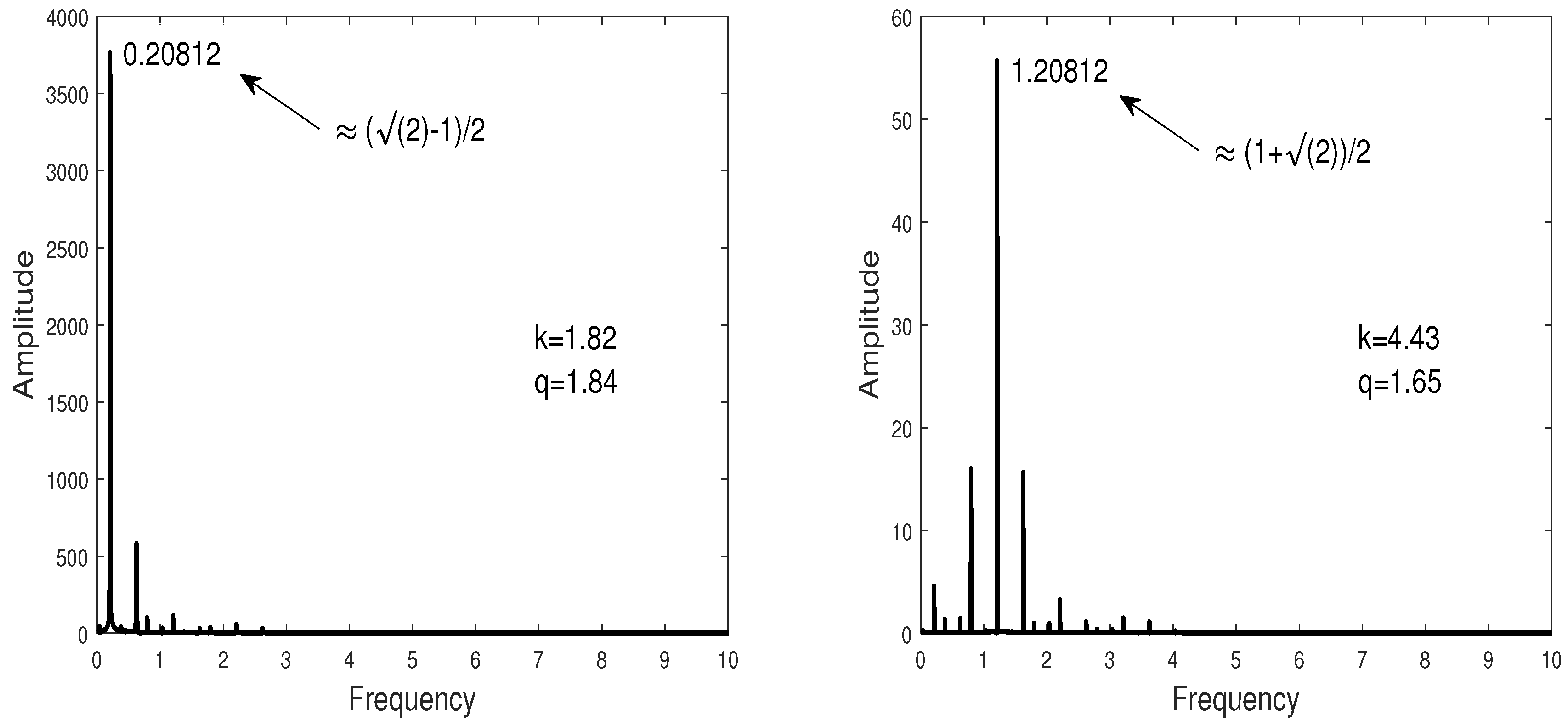
4.2.2. Parametric Resonances
4.3. Effect of the Irrational Frequency Ratio in the Case of Equal Amplitudes of Superimposed Displacements,
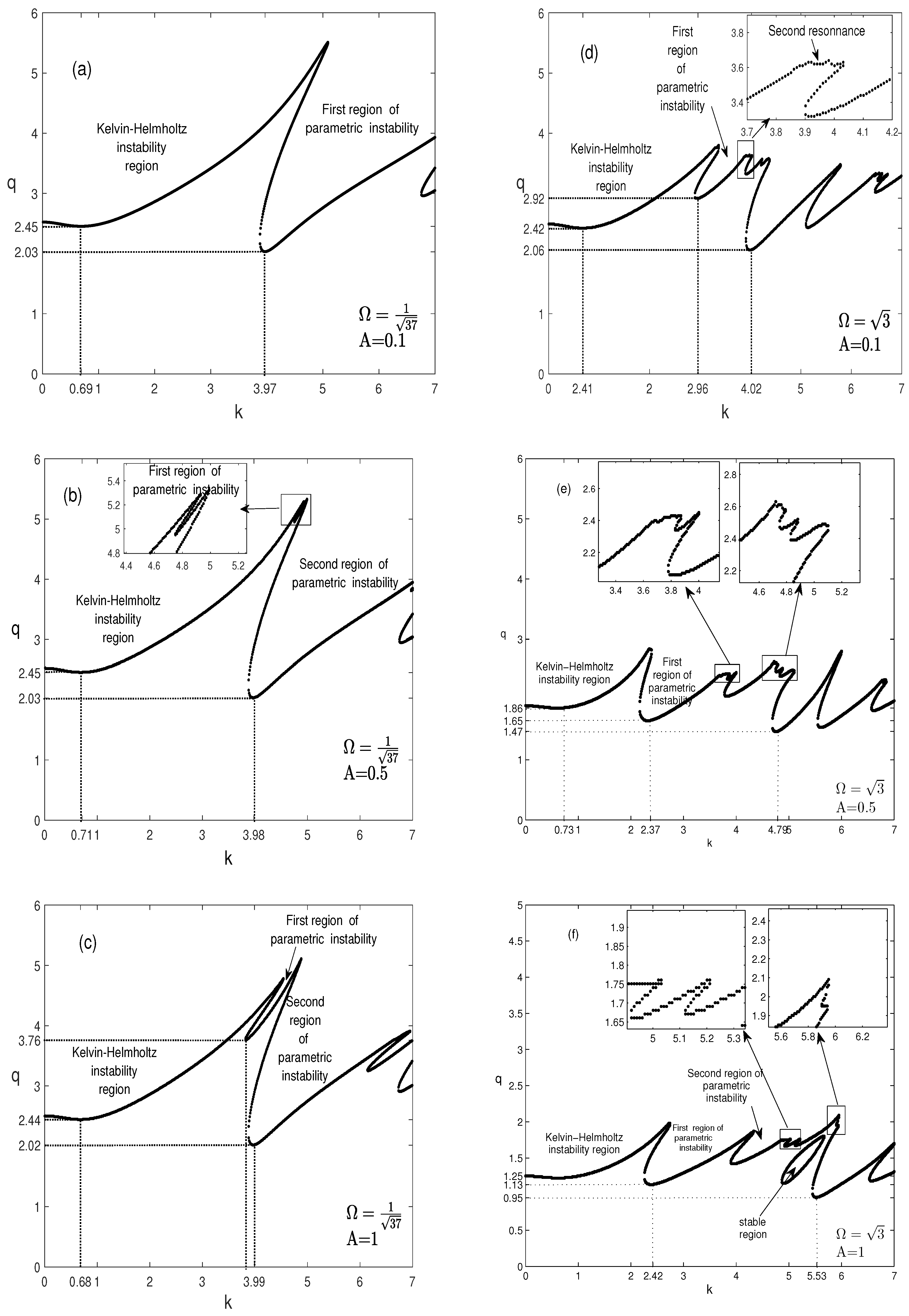
4.4. Effect of the Dimensionless Amplitude of Oscillation A for Different Irrational Ratio of Frequencies
4.5. Effect of the Damping Coefficient F
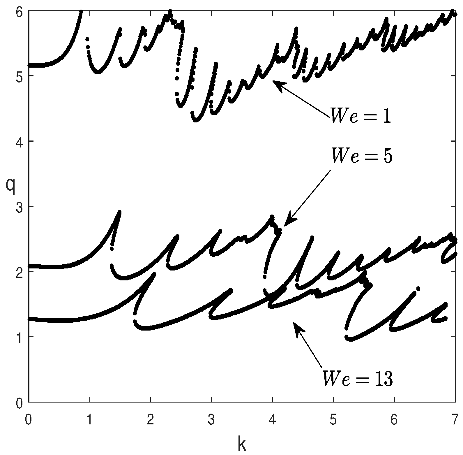
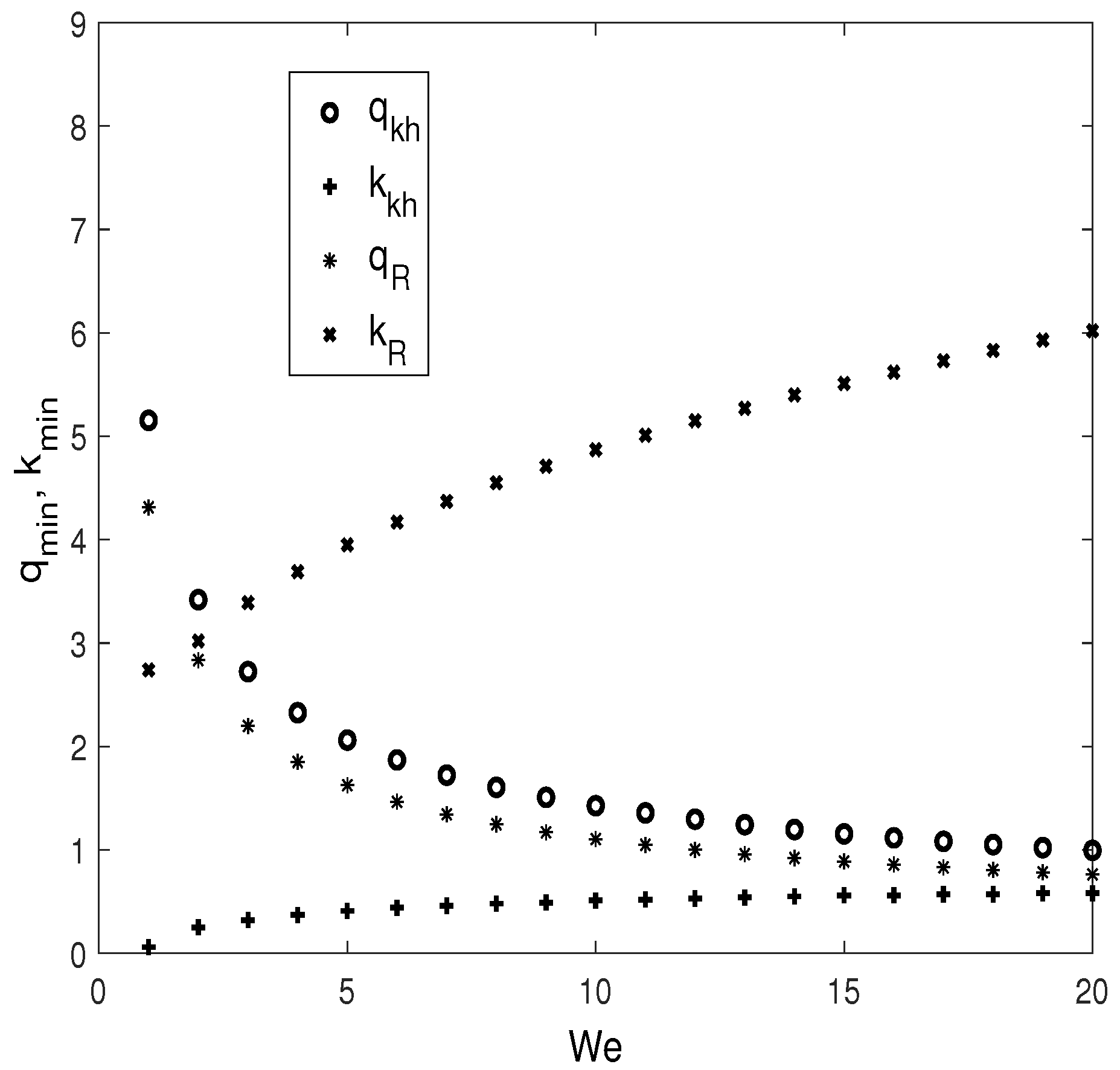
4.6. Effect of the Weber Number, , on the Stability Threshold
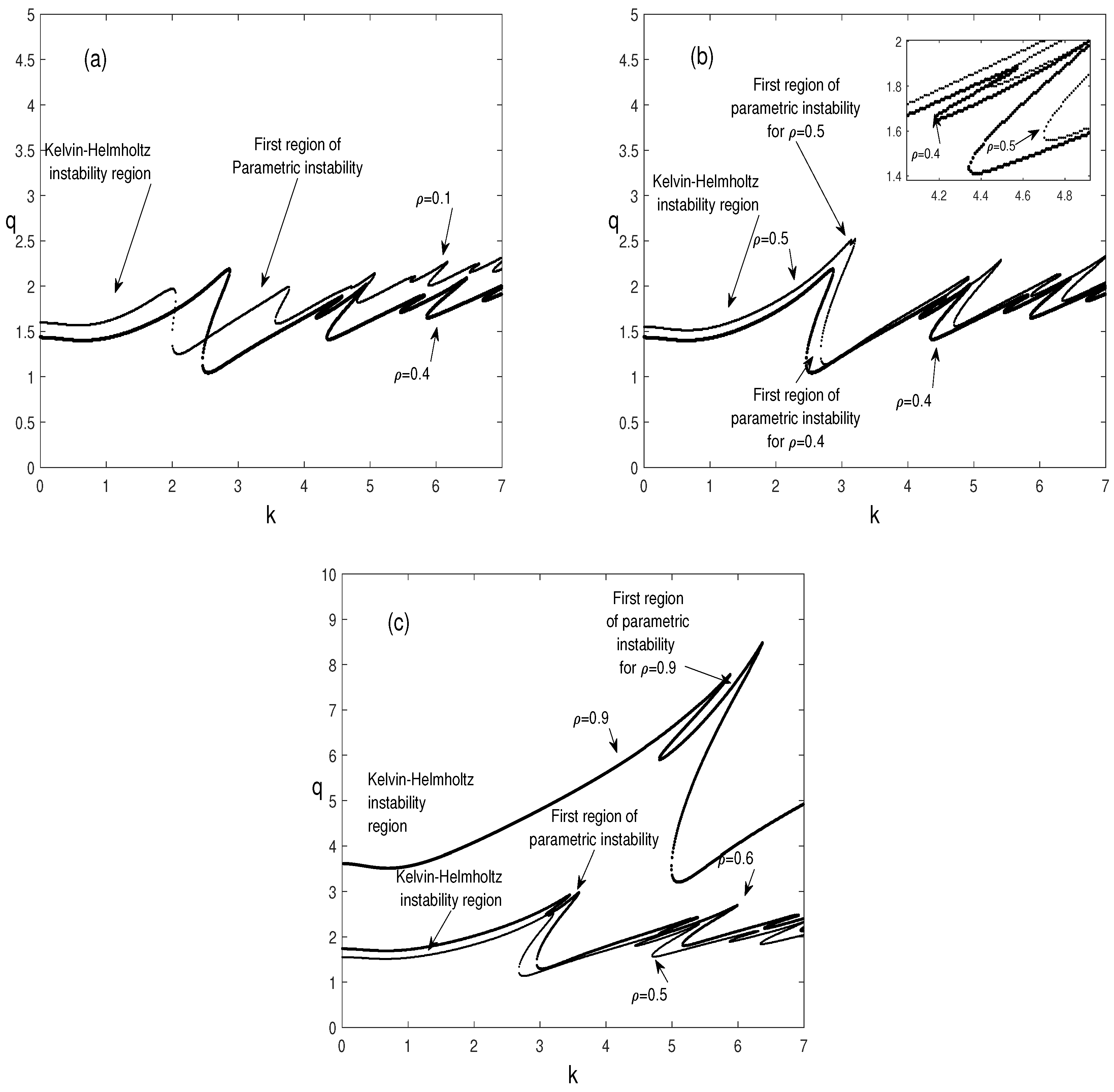
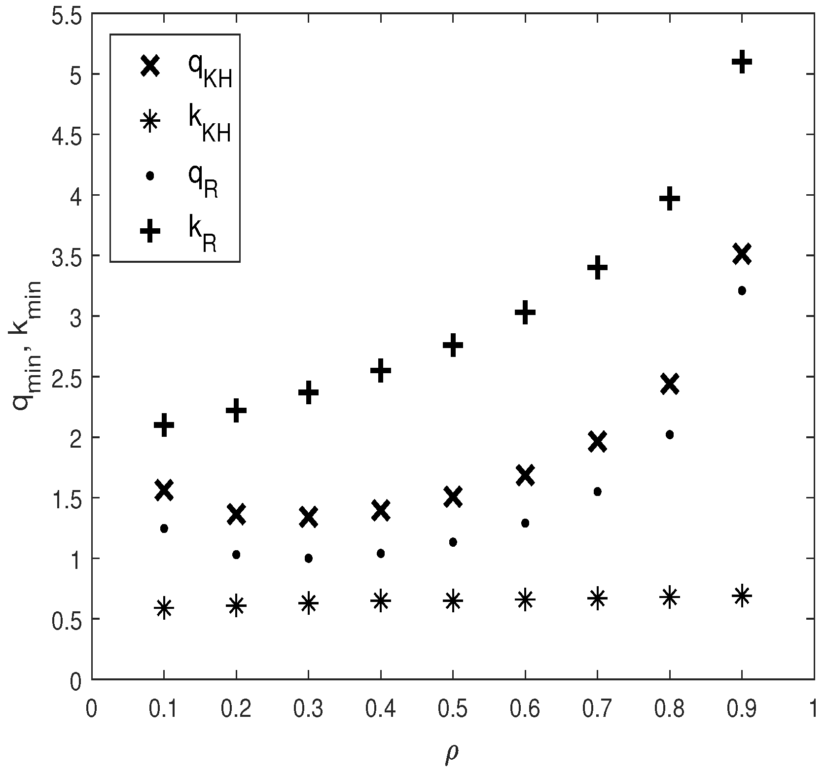
4.7. Effect of the Density Ratio
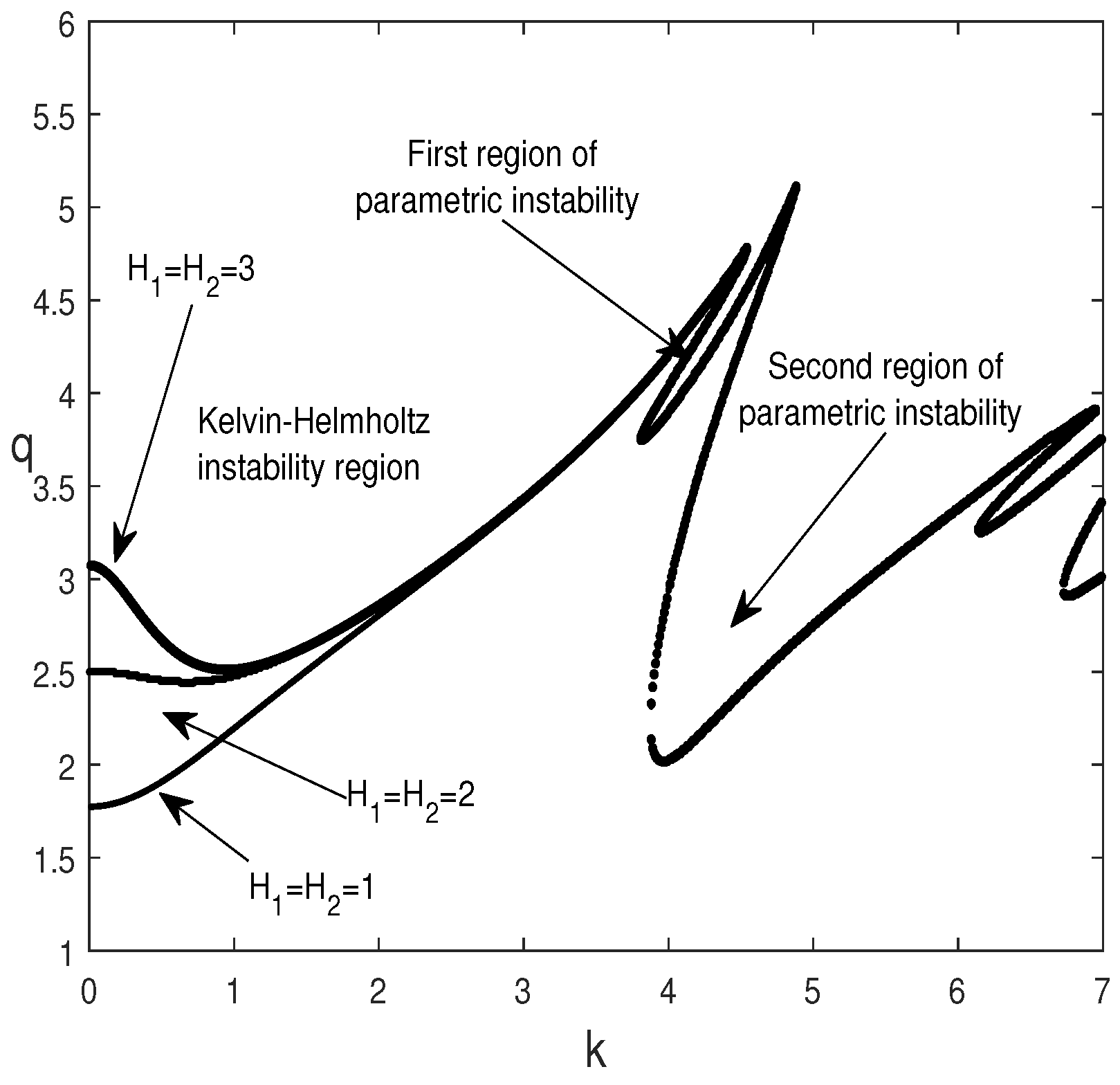
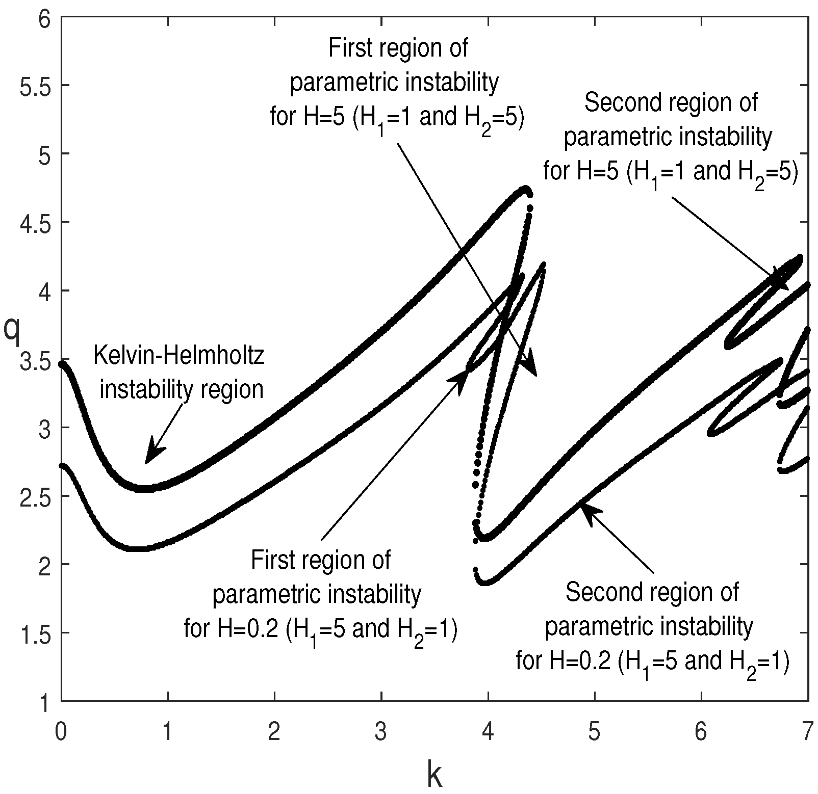
4.8. Effect of the Heights of the Two Fluid Layers and
5. Conclusions
Author Contributions
Funding
Conflicts of Interest
References
- Kelly, R.E. The stability of an unsteady Kelvin–Helmholtz flow. J. Fluid Mech. 1965, 22, 547–560. [Google Scholar] [CrossRef]
- Wolf, G.H. The dynamic stabilization of the Rayleigh-Taylor instability and the corresponding dynamic equilibrium. Z. Phys. A Hadron. Nucl. 1969, 227, 291–300. [Google Scholar] [CrossRef]
- Wolf, G.H. Dynamic Stabilization of the Interchange Instability of a Liquid-Gas Interface. Phys. Rev. Lett. 1970, 24, 444–446. [Google Scholar] [CrossRef]
- Lyubimov, D.V.; Khenner, M.V.; Shotz, M.M. Stability of a fluid interface under tangential vibrations. Fluid Dyn. 1998, 33, 318–323. [Google Scholar] [CrossRef]
- Khenner, M.V.; Lyubimov, D.V.; Belozerova, T.S.; Roux, B. Stability of plane-parallel vibrational flow in a two-layer system. Eur. J. Mech.—B Fluids 1999, 18, 1085–1101. [Google Scholar] [CrossRef]
- Ivanova, A.A.; Kozlov, V.G.; Tashkinov, S.I. Interface dynamics of immiscible fluids under circularly polarized vibration (experiment). Fluid Dyn. 2001, 36, 871–879. [Google Scholar] [CrossRef]
- Talib, E.; Jalikop, S.V. The influence of viscosity on the frozen wave instability: Theory and experiment. J. Fluid Mech. 2007, 584, 45–68. [Google Scholar] [CrossRef]
- Talib, E.; Juel, A. Instability of a viscous interface under horizontal oscillation. Phys. Fluids 2007, 19, 092102. [Google Scholar] [CrossRef]
- Yoshikaway, H.N.; Wesfreid, J.E. Oscillatory Kelvin–Helmholtz instability. Part 1. A viscous theory. J. Fluid Mech. 2011, 675, 223–248. [Google Scholar] [CrossRef]
- Yoshikaway, H.N.; Wesfreid, J.E. Oscillatory Kelvin–Helmholtz instability. Part 2. An experiment in fluids with a large viscosity contrast. J. Fluid Mech. 2011, 675, 249–267. [Google Scholar] [CrossRef]
- Jalikop, S.V.; Juel, A. Oscillatory transverse instability of interfacial waves in horizontally oscillating flows. Phys. Fluids 2012, 24, 044104. [Google Scholar] [CrossRef]
- Bouchgl, J.; Aniss, S.; Souhar, M. Interfacial instability of two superimposed immiscible viscous fluids in a vertical Hele-Shaw cell under horizontal periodic oscillations. Phys. Rev. E 2013, 88, 023027. [Google Scholar] [CrossRef] [PubMed]
- Lyubimova, T.P.; Lyubimov, D.V.; Sadilov, E.S.; Popov, D.M. Stability of the fluid interface in a Hele-Shaw cell subjected to horizontal vibrations. Phys. Rev. E 2017, 96, 013108. [Google Scholar] [CrossRef] [PubMed]
- Li, X.; Li, X.; Liao, S. Observation of two coupled Faraday waves in a vertically vibrating Hele-Shaw cell with one of them oscillating horizontally. Phys. Fluids 2018, 30, 012108. [Google Scholar] [CrossRef]
- Bouchgl, J.; Aniss, S. Effect of Periodic Oscillation on the Interfacial Instability of Two Superposed Fluid Layers in a Fully Saturated Porous Media. Int. J. Appl. Mech. 2021, 13, 2150088. [Google Scholar] [CrossRef]
- Rand, R.; Zounes, R.R.; Hastings, R. Dynamics of a Quasiperiodically Forced Mathieu Oscillator. In Nonlinear Dynamics: The Richard Rand 50th Anniversary Volume; Guran, A., Ed.; World Scientific: Hackensack, NJ, USA, 1997; Chapter 9. [Google Scholar]
- Boulal, T.; Aniss, S.; Belhaq, M.; Rand, R. Effect of quasiperiodic gravitational modulation on the stability of a heated fluid layer. Phys. Rev. E 2007, 76, 056320. [Google Scholar] [CrossRef] [PubMed]
- Boulal, T.; Aniss, S.; Belhaq, M.; Azouani, A. Effect of quasi-periodic gravitational modulation on the convective instability in Hele-Shaw cell. Int. J.-Non-Linear Mech. 2008, 43, 852–857. [Google Scholar] [CrossRef]
- Yagoubi, M.; Aniss, S. Effect of vertical quasi-periodic vibrations on the stability of the free surface of a fluid layer. Eur. Phys. J. Plus 2017, 132, 1–13. [Google Scholar] [CrossRef]
- El Jaouahiry, A.; Aniss, S. Linear stability analysis of a liquid film down on an inclined plane under oscillation with normal and lateral components in the presence and absence of surfactant. Phys. Fluids 2020, 32. [Google Scholar] [CrossRef]
- Gondret, P.; Rabaud, M. Shear instability of two-fluid parallel flow in a Hele-Shaw cell. Phys. Fluids 1997, 9, 3267–3274. [Google Scholar] [CrossRef]
- Nayfeh, H.; Mook, D. Nonlinear Oscillation; WILEY-VCH Verlag GmbH and Co. KGaA: Weinheim, Germany, 2004; pp. 276–296. [Google Scholar] [CrossRef]


Disclaimer/Publisher’s Note: The statements, opinions and data contained in all publications are solely those of the individual author(s) and contributor(s) and not of MDPI and/or the editor(s). MDPI and/or the editor(s) disclaim responsibility for any injury to people or property resulting from any ideas, methods, instructions or products referred to in the content. |
© 2023 by the authors. Licensee MDPI, Basel, Switzerland. This article is an open access article distributed under the terms and conditions of the Creative Commons Attribution (CC BY) license (https://creativecommons.org/licenses/by/4.0/).
Share and Cite
Assoul, M.; El jaouahiry, A.; Bouchgl, J.; Echchadli, M.; Aniss, S. Effect of Horizontal Quasi-Periodic Oscillation on the Interfacial Instability of Two Superimposed Viscous Fluid Layers in a Vertical Hele-Shaw Cell. Fluids 2023, 8, 164. https://doi.org/10.3390/fluids8060164
Assoul M, El jaouahiry A, Bouchgl J, Echchadli M, Aniss S. Effect of Horizontal Quasi-Periodic Oscillation on the Interfacial Instability of Two Superimposed Viscous Fluid Layers in a Vertical Hele-Shaw Cell. Fluids. 2023; 8(6):164. https://doi.org/10.3390/fluids8060164
Chicago/Turabian StyleAssoul, Mouh, Abdelouahab El jaouahiry, Jamila Bouchgl, Mourad Echchadli, and Saïd Aniss. 2023. "Effect of Horizontal Quasi-Periodic Oscillation on the Interfacial Instability of Two Superimposed Viscous Fluid Layers in a Vertical Hele-Shaw Cell" Fluids 8, no. 6: 164. https://doi.org/10.3390/fluids8060164