Article

Stream and Potential Functions for Transient Flow Simulations in Porous Media with Pressure-Controlled Well Systems

1
Department of Mathematics, College of Computing and Mathematics, King Fahd University of Petroleum & Minerals (KFUPM), Dhahran 31261, Saudi Arabia
2
Center for Integrative Petroleum Research (CIPR), King Fahd University of Petroleum & Minerals (KFUPM), Dhahran 31261, Saudi Arabia
3
Department of Petroleum Engineering, College of Petroleum Engineering and Geosciences (CPG), King Fahd University of Petroleum & Minerals (KFUPM), Dhahran 31261, Saudi Arabia
*
Authors to whom correspondence should be addressed.
Fluids 2023, 8(5), 160; https://doi.org/10.3390/fluids8050160
Submission received: 20 March 2023 / Revised: 14 May 2023 / Accepted: 15 May 2023 / Published: 17 May 2023

Abstract

:
Gaussian solutions of the diffusion equation can be applied to visualize the flow paths in subsurface reservoirs due to the spatial advance of the pressure gradient caused by engineering interventions (vertical wells, horizontal wells) in subsurface reservoirs for the extraction of natural resources (e.g., water, oil, gas, and geothermal fluids). Having solved the temporal and spatial changes in the pressure field caused by the lowered pressure of a well’s production system, the Gaussian method is extended and applied to compute and visualize velocity magnitude contours, streamlines, and other relevant flow attributes in the vicinity of well systems that are depleting the pressure in a reservoir. We derive stream function and potential function solutions that allow instantaneous modeling of flow paths and pressure contour solutions for transient flows. Such analytical solutions for transient flows have not been derived before without time-stepping. The new closed-form solutions avoid the computational complexity of time-stepping, required when time-dependent flows are modeled by superposing steady-state solutions using complex analysis methods.

1. Introduction

Streamline and flow path simulations are routinely used to study fluid migration in a variety of subsurface reservoirs containing water, geothermal, or hydrocarbon resources. Advanced tools exist to model the migration of fluids in subsurface reservoirs, ranging from analytical [1,2,3] to numerical methods such as finite difference and finite element methods [4,5,6]. In addition to modeling fluid migration in the reservoir, finite difference methods are used to numerically solve the transient flow in complex pipe networks [7]. Changjun et al. [8] built a model for both steady-state and transient flow in condensate gas pipelines and solved the problem using a fourth-order Runge-Kutta method and the Gaussian elimination method. Tong et al. [9] studied the behavior of the wellhead pressure for transient non-isothermal wellbore flow. Agaie et al. [10] considered the variation of pressure, velocity, density, and temperature with respect to time in the simulation of transient gas flow. In [11], a mathematical model was developed for nonisothermal inflow and lifting of the recovered geothermal fluid, which was solved numerically using a fourth-order Runge-Kutta method.
Although numerical methods are widely used and provide efficient solutions for simulating transient flow in the studies cited [4,5,6,7,8,9,10,11] (and many others), analytical solutions for transient flow [1,2,3] aim to avoid the complexity and resolution issues of gridding that are associated with the numerical methods. Numerical tools require gridding and meshing, which makes them relatively complex to use (involving the translation of partial differential equations into numerical solution scheme format). In addition, computation times for sensitivity studies and well-placement optimization using numerical solution methods are relatively time-consuming (and therefore costly) as compared to closed-form solution methods.
Numerous analytical solutions (both approximations and exact solutions) for transient flow have been proposed in earlier studies. For example, Wu and Pan [12,13] presented a set of analytical solutions for transient flow in unsaturated porous media. Lu et al. [14] presented approximate analytical solutions for transient gas flow from a vertically fractured well, which can be efficiently used to evaluate the fractured reservoir properties. Amadei et al. [15] considered the effects of non-Newtonian Bingham viscoplastic fluids and provided analytical solutions for the non-transient flow of Bingham viscoplastic materials in rock fractures. Analytical methods based on complex analysis methods (CAMs) combined with time-stepping provide fast alternatives to visualize the streamlines and time-of-flight contours [1]. The basic solution method assumes flow in unbounded domains, but conformal mapping allows for flow path construction of flood displacement fronts in the presence of reservoir boundaries [2].
The present study further explores the potential of a fast-analytical method to model transient fluid flow in porous media that computes the local pressure gradient using Gaussian pressure transients (GPT) [16,17]. The GPT method is briefly explained and illustrated in Section 2. Although the GPT solution was presented first by Weijermars [16] for the pressure diffusion equation, the diffusion-convection equation is at the basis of the GPT solutions. One of the findings in [16] was that not only the diffusive mass transport due to molecular (self) diffusion can be modeled with the Gaussian solution, but also the advective (or convective) mass transport due to pressure gradients can be modeled with such Gaussian solutions. This unified solution was further elaborated in [18], introducing a Peclet number defined as the ratio of the advective mass transport and diffusive mass transport. For Pe > 1, the advection advanced faster than the molecular diffusion; for P < 1, the reverse holds: molecular diffusion dominates the mass transfer process.
After solving the scalar pressure field in the reservoir space, Darcy’s Law is applied in the present study to directly compute the fluid flux from the reservoir into the well system. The method can also be used to compute vector-field-based flow paths as the fluid moves from the porous reservoir rock into hydraulically fractured well systems.
The ultimate aim of flow path simulations is commonly two-fold: (1) to predict the fluid extraction rate (well productivity) based on the flux of fluid through stream tubes toward the producer well, and (2) to study where in the reservoir that fluid originated from. While many studies focus on the fluid extraction from reservoirs (e.g., water, oil, gas, and geothermal fluids), additional applications include fluid injection for either disposal or storage of certain fluids (such as waste fluids, carbon dioxide, hydrogen, natural gas, etc.). For such cases, the solution methods presented here are equally valid; a sign conversion can be applied to model the well injectivity using a certain pressure required to maintain a certain flux in the injection wells.
The results for pressure transients propagating from the selected well constellations, generated with Gaussian pressure transients (GPT), are validated in the present study against known solutions computed with a suitable separate solution method. For example, the gridless and meshless complex analysis method (CAM) used in prior studies of flow in subsurface reservoirs [1,2,3,19,20,21,22] can model flow paths under steady-state conditions, augmented with time-stepping to account for wells of variable strength (the CAM pressure field is static at each time step, without a true time-dependent pressure transient as its basis).
In contrast to CAMs, GPT solutions can show the flow paths for both the transient period and a subsequent steady-state flow period; the steady-state will only occur when injection and production volumes are balanced. The comparison between CAMs and GPT solutions is evaluated by constructing the flow paths for vertical well arrangements with regular spacing between them using 2-, 5-, and 7-spot well pattern arrangements (Figure 1), essentially benchmarking GPT solutions for these well constellations. Next, GPT solutions are used to derive new explicit, analytical solutions for the stream function and potential function describing the time-dependent flow paths, which will shift spatially during the transient flow period (Section 4).
Analytical stream and potential function solutions in the domain of complex analysis and complex potentials are limited to steady-state flow and can only account for time-dependency by superposing steady-state solutions with small incremental time-steps. The accuracy of such solutions is determined by the product of the local velocity and the duration of the finite time-step, which may lead to inaccuracy in spite of using the closed-form CAM solution [19,20,21]. In the present work, new GPT solutions allow us to visualize the solutions of the stream and potential functions for both the steady-state and transient stages of flow development. Furthermore, deriving stream and potential functions from only the imposed bottomhole pressures of the well system used for the extraction of natural resources, including oil, gas, and water, from subsurface reservoirs provides a very powerful new tool because it can be used to optimize the well positioning, adjust pressures if well rates become sub-economic, and find the optimum solution, all of which will contribute to more efficient and sustainable utilization of natural resources.
The present study proceeds as follows: Section 2 lists the basic assumptions used in the Gaussian pressure field solution for reservoirs with either isotropic or anisotropic diffusivity. For a reservoir with a single well (producer or injector), the depletion of the reservoir pressure evolves as the pressure transient advances and will continue indefinitely. For reservoirs with multiple sources of pressure change, the pressure gradient in the reservoir region between the wells will reach a steady state. Section 3 benchmarks the flow path solutions against known solutions obtained with independent analytical CAM solutions, using the same initial conditions and a variety of well systems. Section 4 presents new solutions for the stream function and potential function for transient flow, which can then be used to visualize the streamlines and equipotential lines at different times. A discussion follows in Section 5, and conclusions are given in Section 6.

2. Methodology

This section introduces the key elements used in our models. First, we explain the basic assumptions (Section 2.1), the equation of motion governing the flow in porous media (Section 2.2), the Gaussian pressure transient (GPT) equations, and examples of GPT solutions (Section 2.3). Next, it is detailed how pressure transients evolve (Section 2.4) after injection and production wells are started with an instantaneous change in the bottomhole pressure (PBH) after such wells are switched on in either a production or injection mode, or when multiple wells operate in combinations thereof.

2.1. Basic Assumptions

In the Gaussian solution of the pressure-diffusivity equation, the hydraulic diffusivity is the key controlling parameter for all fluid transfer [16,17]. This approach turns out to greatly simplify the computation of pressure transient solutions for a wide range of practical applications. In this study, the fluid transfer in hypothetical reservoirs will be modeled based on the following initial assumptions:
  • The porous medium hosting the reservoir is considered homogeneous and possesses either isotropic or anisotropic diffusivity.
  • The fluid flow in the reservoir is solely due to pressure gradients caused by engineering interventions (such as the drilling of injection and production wells), where a lowered bottomhole pressure is maintained by the production system at the reservoir inflow level.
  • The fluid in the reservoir is assumed to be single-phase, incompressible (variations in density are negligible), isotropic (the properties are not dependent on the direction along which they are measured), and of Newtonian viscosity (the viscosity does not change when we apply a stress and its magnitude is insensitive to pressure changes).

2.2. The Fluid Motion Model in a Porous Medium

The motion of the fluid can be described by the Navier-Stokes equation (see [23]), which assumes the fluid is practically incompressible:
ρ ( u t + ( u ) u ) = P + ρ g + μ 2 u ( Balance   of   momentum ) ,
u = 0 ( Incompressibility   condition ) .
In Equation (1a,b):
  • u = u ( x , y ,   t )   is the fluid velocity, where ( x , y )   in two dimensions is the spatial coordinate and t is the time variable.
  • ρ   is the fluid density, and μ   is the fluid viscosity, and they are assumed constants as stated in Section 2.1.
  • P = P ( x , y ,   t ) is a scalar function representing the pressure of the fluid in every spatial location (x, y), and at any time t; g is gravity’s acceleration, which is needed when the gravity forces are included in the analysis, such as in buoyancy-driven flows due to thermal gradients.
  • The gradient operator in 2D is = ( x , y ) , and the Laplace operator is 2 = 2 x 2 + 2 y 2 .
  • The term ( u ) u is called the convection term, and the term μ 2 u is the diffusion term. Therefore, Equation (1a) belongs to the class of convection–diffusion equations.
  • Equation (1b) is the mass conservation equation, also called the continuity equation in the case of incompressible flow (i.e., with a constant density ρ ). Note that in practice, the equation of motion for incompressible fluids is still found to be applicable to slightly compressible fluids (such as oil and gas-saturated oils).
The right-hand side of Equation (1a) represents the various forces acting on the fluid body: (1) the pressure force, which drives the motion; (2) the body force, which is due to gravity; and (3) the viscous force, which resists the fluid motion. The left-hand side of Equation (1a) represents the time-dependent changes in velocity (in the first term) and convective acceleration (in the second term). The convection term makes Equation (1a) nonlinear, and hence a closed-form solution is applicable only under special conditions. For example, if we assume the convection acceleration is small enough to be neglected (i.e., ( u ) u   0 ), ignoring the body force, only the pressure-driven flow term of Equation (1a) remains, which then simplifies as follows:
μ 2 u P = 0 .
For a porous medium, Equation (2) is solved at a macroscopic scale, considering the properties of the porous medium, such as the porosity, ϕ i j , and the permeability tensor, κ i j . The fluid velocity u r (in m2s−1), due to a given pressure gradient in a porous medium, is given by:
u r ( x , y , t ) = κ i j ϕ i j μ P ( x , y , t ) .
The derivation of Equation (3a) from Equation (2) is obtained by averaging over a cross section of the flow tube representing the pore space in the medium (see [23]). If we remove the porosity,   ϕ i j , from Equation (3a), we will obtain the fluid flux (also called the Darcy velocity) as it will occur at the reservoir level into the well system:
q D = κ i j μ P
The relation between the fluid velocity, u r , in the pore space of the reservoir and the Darcy velocity, q D , into the well system is then given by u r   ϕ = q D (see Section 4).
In reservoir models, Equation (3b) quantifies the inflow of fluid into the well system at the reservoir level. The volumetric rate of inflow from the reservoir requires multiplication of the flux rate by the vertical exposure of the wellbore to the reservoir space of thickness h . In addition, hydrocarbons in the reservoir have a different volume than at surface conditions, which is accounted for by the so-called formation volume factor β . The formation volume factor is defined as the ratio of the volume at reservoir conditions divided by the volume at surface conditions. Hence, with isotropic porosity and permeability, the volumetric rate q w of the outflow at the well head (surface level) from a vertical well with radius r w is given by (see [17]):
q w ( x , y , t ) = 2   π   r w h β   κ   μ   P ( x , y , t ) .
In Equation (3c), the parameter κ h represents the reservoir conductivity, which governs how fast fluid can flow from the reservoir to the wellhead. If we only study the pressures in the reservoir, we do not need to convert them to fluid volumes produced at surface conditions ( β can be conveniently dropped). Neither do we need to multiply with reservoir thickness (h can be conveniently dropped) if we confine our analysis to flow in a horizontal plane (map view) at the reservoir level. The radius of the well is only needed in the expression when we aim to compute the volumes collected at the well (so 2   π   r w can be dropped as well). We retain for our initial analysis the fluid flux (Darcy velocity) formula of Equation (3a), which describes fluid mass transfer in the reservoir space.
Another crucial simplifying step made here is that rather than modeling with the dimensional hydraulic diffusivity, the present study uses normalized quantities (see Appendix A), which speeds up the subsequent computations. However, for translation to any real well cases, properly scaled dimensional inputs should be used.
In our presented work, Equation (3a) is used to compute the fluid flux (Darcy velocity) from the reservoir into the well system and any hydraulic fractures, and then we plot the flow paths. Although well-known numerical grid-based methods can be used to solve Equation (3a), they have limited resolution compared to analytic solutions. To solve Equation (3a) analytically, we need to know what the pressure gradient is everywhere in the reservoir due to the pressure disturbance and its transient advance caused by the well system. The spatial and temporal pressure gradients can be solved by the Gaussian pressure transient method introduced in Weijermars [16].

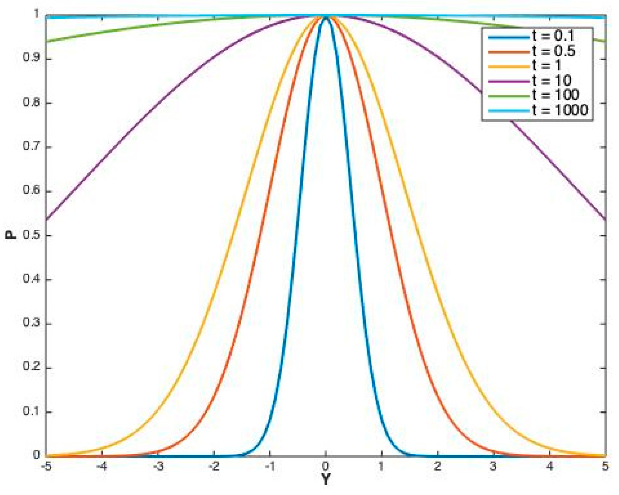
2.3. Gaussian Pressure Transient Solution

The 1D pressure diffusion equation is [16,17]:
P t = D h ( 2 P x 2 ) ,
where D h represents the hydraulic diffusivity and is assumed to be homogenous throughout this study. However, in reservoir studies, we are commonly dealing with a pre-existing pressure in the reservoir, P 0 , which is then suddenly changed by an engineering intervention (e.g., producer wells and hydraulic fractures). Thus, a local pressure change is commonly imposed. We therefore define a local pressure change as:
Δ P 0 = P 0 P B H
where P B H is the bottomhole pressure in the well system. Equation (4) can now be rewritten as:
Δ P t = D h ( 2 Δ P x 2 ) .
The Gaussian 1D-diffusion solution as presented in [16] is then given by:
Δ P ( x , t ) = Δ P 0   e x 2 4 D h t .
The boundary condition is an assumed constant P B H . Equation (7) can now be used for tracking the spatial and temporal change of the pressure due to a unidirectional 1D-pressure diffusion in a reservoir layer, which shows how the pressure front advances from a planar source (such as a hydraulic fracture) into the reservoir along the x-direction. Below, we visualize Gaussian solutions for 2D-diffusion cases (such as those applicable to reservoirs produced with vertical wells) with (1) isotropic diffusivity (Case A) and (2) anisotropic diffusivity (Case B).
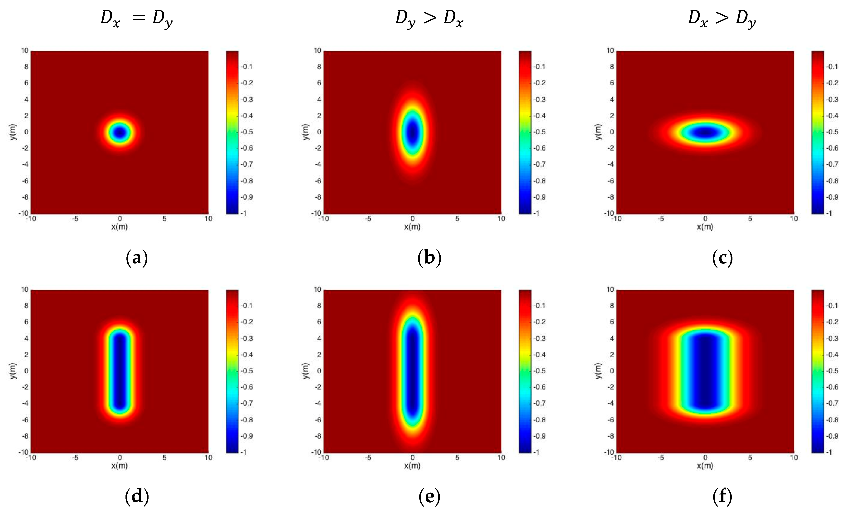
  • Case A: Isotropic diffusivity
When the reservoir diffusivity is the same in every direction (for 2D and 3D diffusion sources), the diffusivity can be represented by a scalar D h . The solutions for the spatial and temporal change of the pressure for 2D and 3D isotropic pressure diffusion are [16]:
Δ P ( x , y , t ) = Δ P 0 e ( x 2 + y 2 4 D h t )                                                       ( for   2 D difussion ) ,
Δ P ( x , y , z , t ) = Δ P 0 e ( x 2 + y 2 + z 2 4 D h t )                                       ( for   3 D difussion ) .
Figure 2b presents a Gaussian pressure transient solution for   2 D -diffusion in a horizontal reservoir produced with a single vertical well (Figure 2a) using Equation (8a). The vertical scale in Figure 2b shows the pressure transient probability profile starting from the pressure drop source. For simplicity, the isotropic pressure diffusivity D h was non-dimensionalized (see Appendix A) in such a way that D h = 1 . For the single vertical well (Figure 2a,b), the pressure transient contours will advance in the reservoir, expanding as concentric circles of radius r = x 2 + y 2 in a 2D map view (Figure 3a) and as a cone in a 3D perspective (Figure 2b). The reservoir pressure drop Δ P 0 in Equation (8a) is entered as a negative z -value. Further away from the pressure drop source, Δ P ( x , y , t ) = 0 , if the time used is relatively short as compared to the diffusion rate, which means that there is no pressure change in the region further away from the pressure drop source (red top surface in Figure 2b).
The solution for a finite-length, single hydraulic fracture (Figure 2c) was constructed by superposing 1D-diffusion (Equation (7)) with the 2D-solution of radial flow (Equation (8a)) for the fracture tips (Figure 2d). Following [16,17], when the transient propagates in all 2D directions away from the initial pressure drop source, a conditional modification is used in all presented examples of pressure diffusion initiated from hydraulic fractures:
  • For y W f , use y y W f ;
  • For W f < y < W f , use y 0 ;
  • For y   W f , use y y + W f .
The pressure change induced by a single hydraulic fracture (Figure 2c,d) of half-length W f in 2D map view is represented by elliptical pressure transient contours (see Figure 3d–f). The GPT solution used in the present study is the approximate solution of Equation (19) in Weijermars [17], while an exact solution is also given as Equation (B18) in that same study [17].
  • Case B: Anisotropic diffusivity
This case considers layered reservoirs in which the hydraulic diffusivity is not a scalar but a tensor quantity sensitive to direction in the (x, y)-plane represented by the 2D-diffusivity tensor, D i j . If we consider the case when D i j = 0 for i j , then the diffusivity in each direction will be denoted by D x and D y . The temporal pressure change in 2D-diffusion space with anisotropic diffusivity is [16]:
Δ P ( x , y , t ) = p ( x , y , t ) Δ P 0 = e 1 4 t ( x 2 D x + y 2 D y ) Δ P 0   ,
where p ( x , y , t ) is the Gaussian probability function [16,17].
Figure 3 shows map views of the pressure transient advance (for certain times) in the target zone originating from a vertical well (top row) and from a horizontal hydraulic fracture (bottom row). The first column of Figure 3 is for the base case model with isotropic diffusivity ( D x = D y ) . The second and third columns of Figure 3 are for anisotropic pressure diffusivity, where the pressure change is computed using Equation (9). For both types of well systems, the pressure contours representing the advance of the pressure transient at a certain time will show stretching in the y -direction if D y > D x (Figure 3b,e), and stretching occurs in the x -direction if D x > D y (Figure 3c,f).

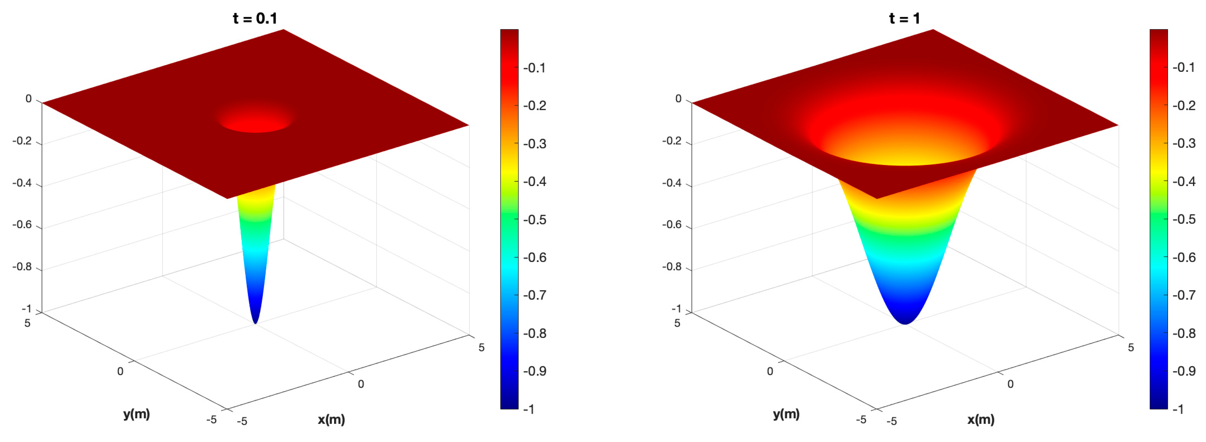
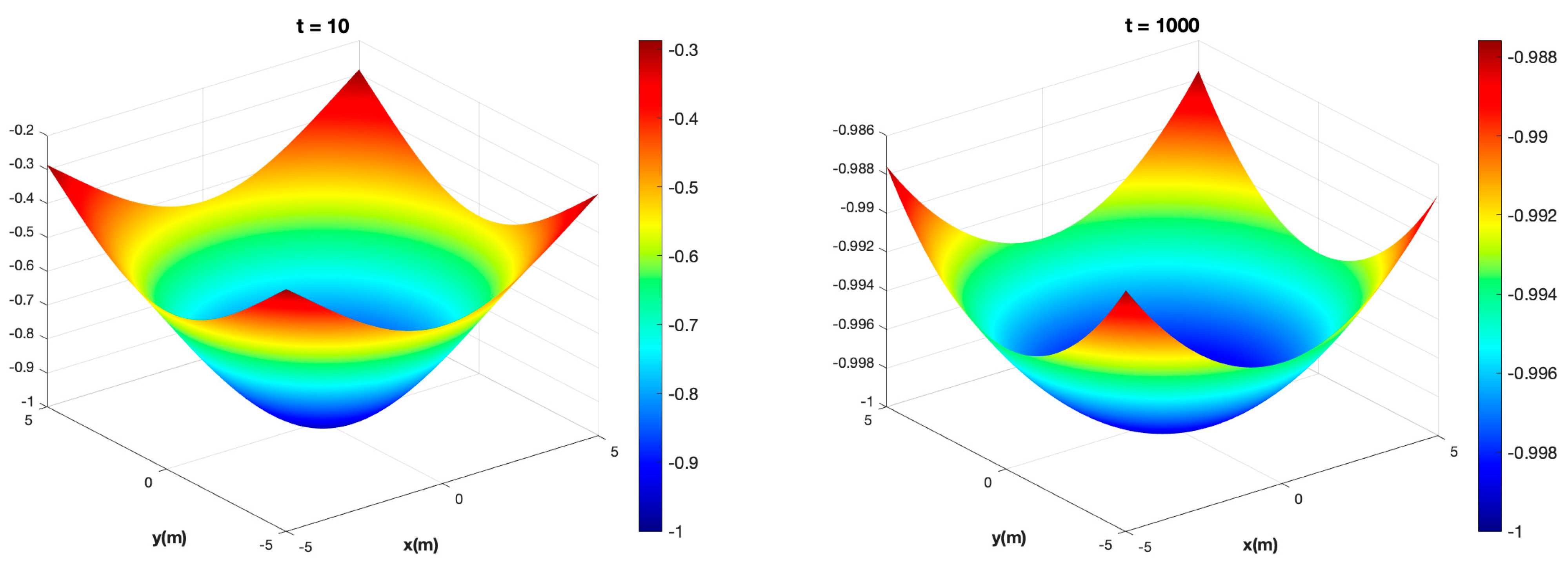
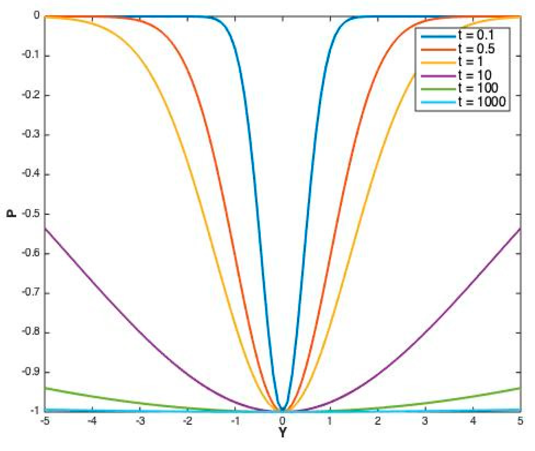
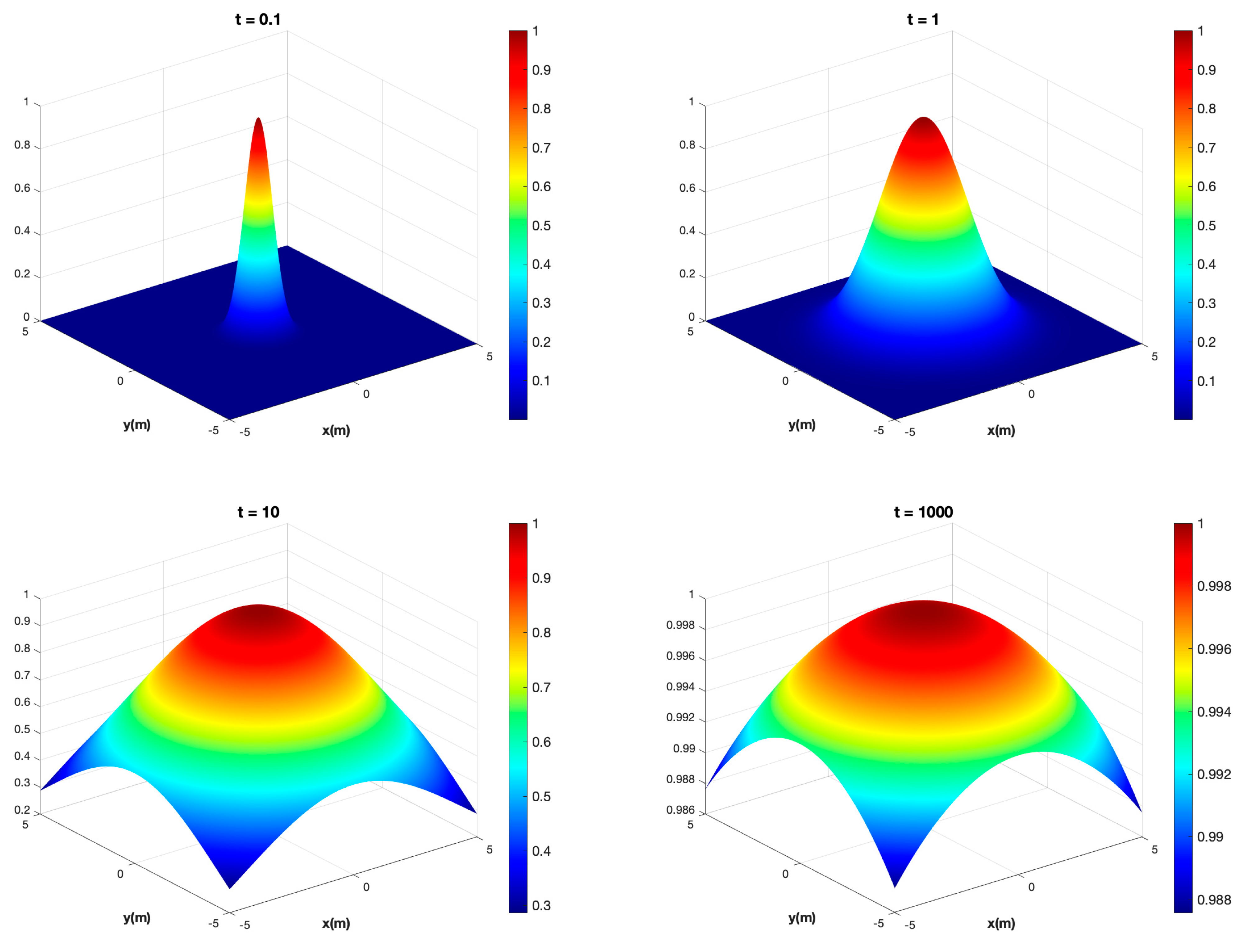
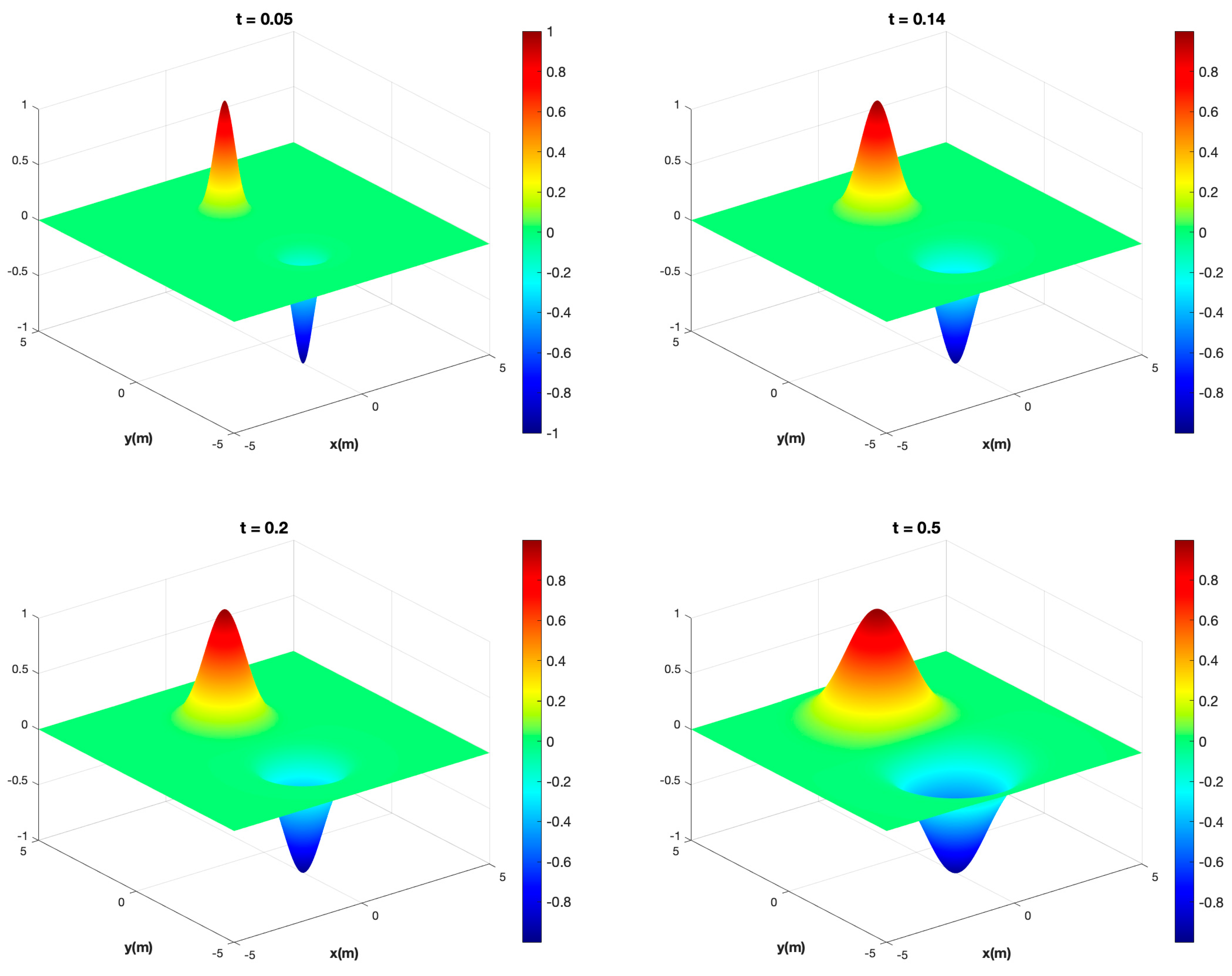
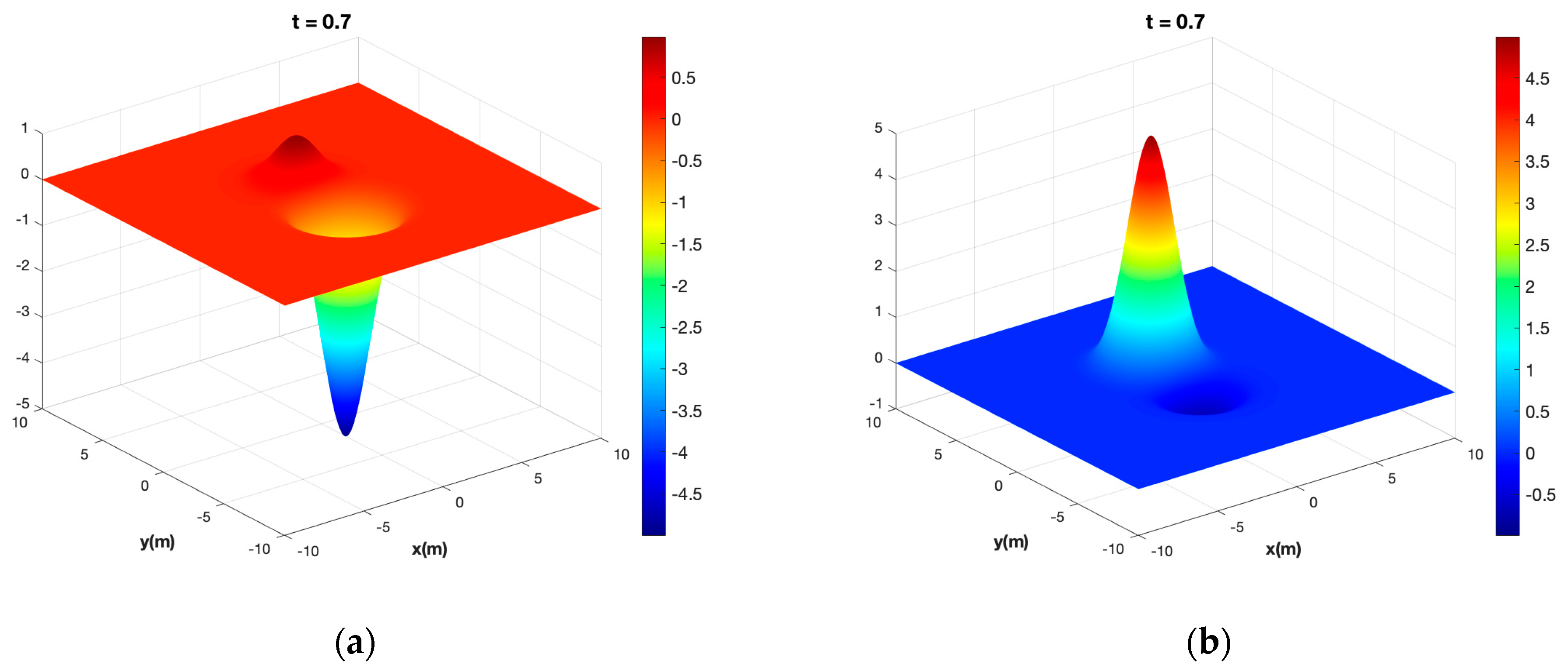
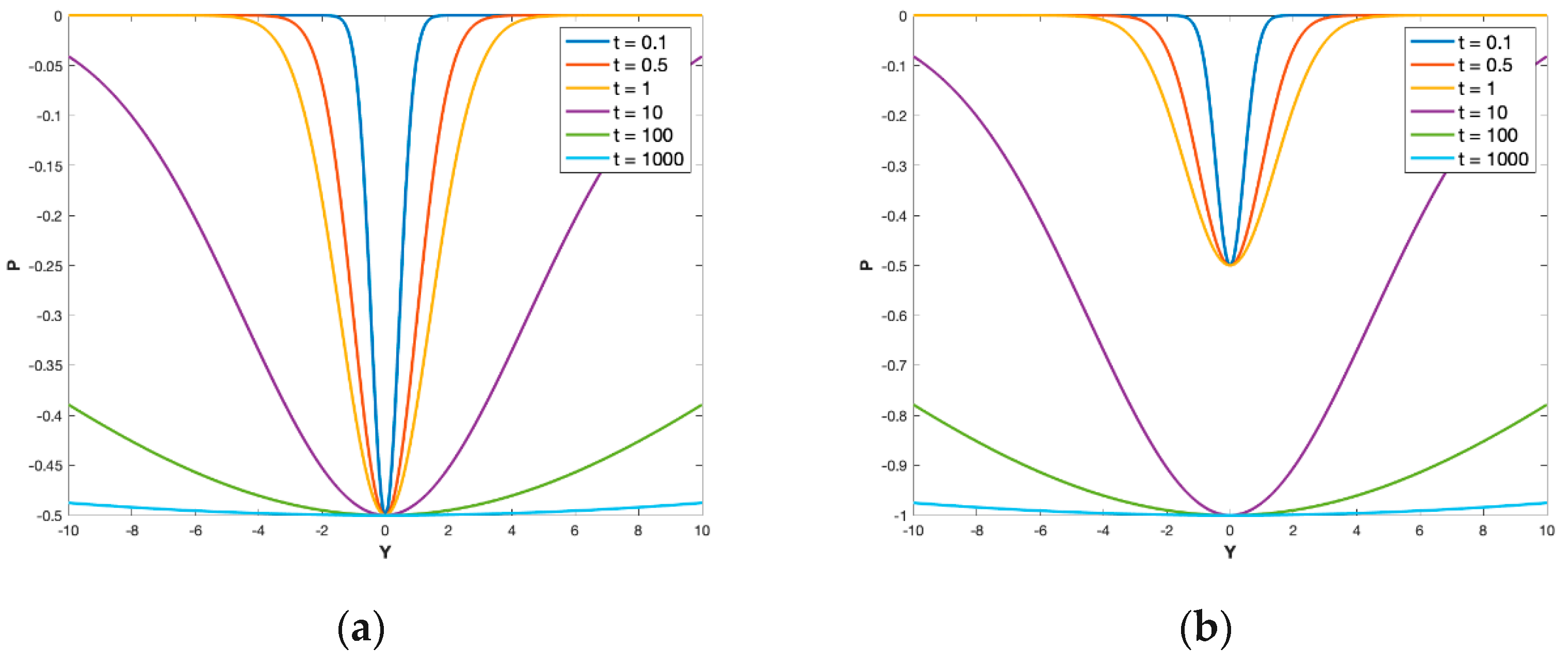
2.4. Evolution of Pressure Transients

The pressure gradient changes with respect to time, P t , and will advance in space until a steady pattern is established sometime after the onset of the pressure disturbance due to the well intervention. As long as flow is still in the transient state, the pressure rate is a function of the well geometry and time variable, P t = F ( x , y , t ) . In regions where the pressure gradient no longer changes with time, P t = 0 , the flow is classified as a steady-state flow.
In this section, we track the Gaussian pressure transient evolution over time until it either ceases altogether due to pressure depletion or reaches a steady state for three illustrative, simple well systems (Figure 4). A single producer (Figure 4a) or a single injector (Figure 4b) will never reach steady-state flow because the pressure transient will advance in the reservoir until the entire reservoir attains the bottomhole pressure (PBH). The reservoir pressure is then said to be depleted, at which point the pressure gradient P will no longer exist, the flow in the reservoir will cease, and the well will stop producing fluid from the subsurface. For cases with one producer and one injector (Figure 4c), a steady-state flow can be locally maintained in the region between the wells after the pressure gradient profile between the well pairs has been established (see below).
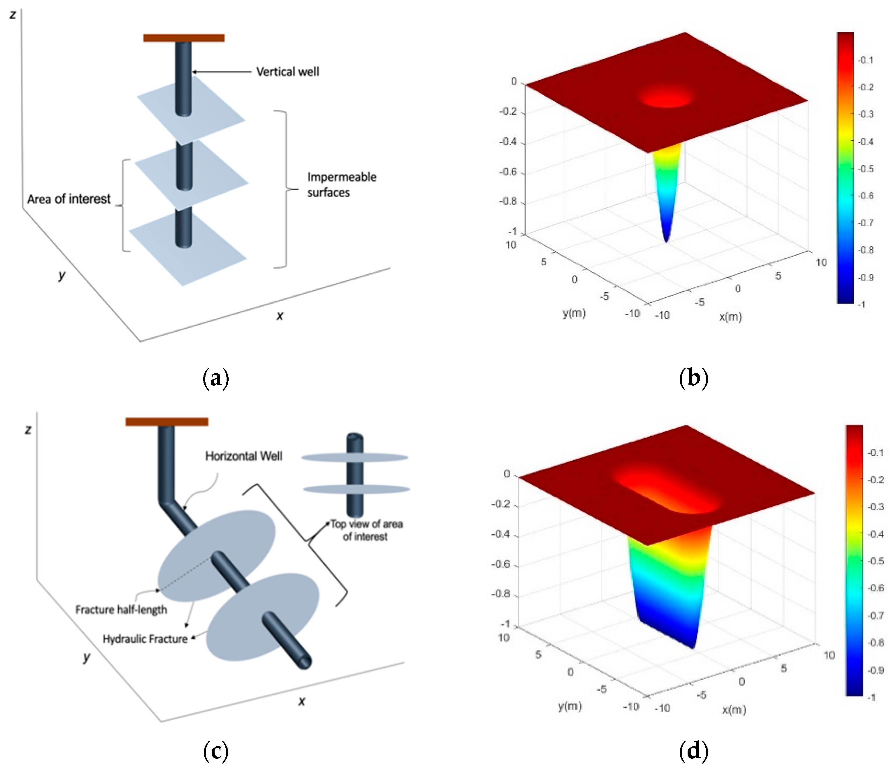
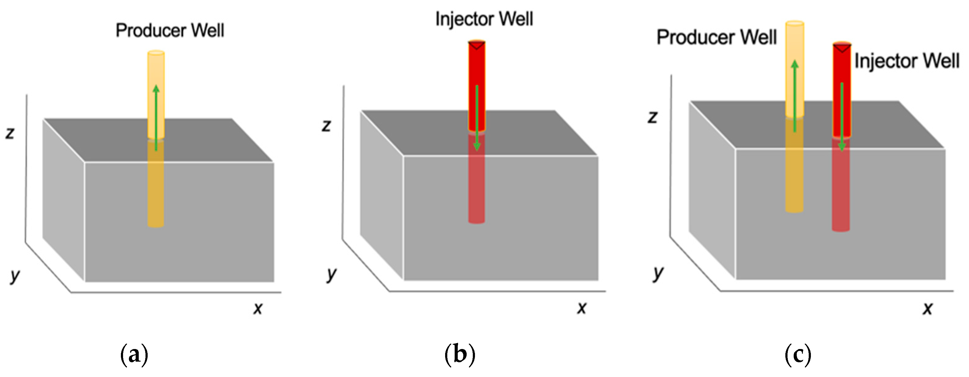
  • Case 1: Reservoir produced with a single vertical well
Gaussian pressure transient solutions are plotted in Figure 5 for a variety of times since the introduction of a pressure perturbation at the bottom of the well. Complete depletion of the reservoir pressure is an asymptotic process and will not occur until time becomes indefinite.
Figure 6 shows the evolution of the pressure depletion profiles at different times as seen in a section containing the producer well located at the origin; as time passes, the pressure in the reservoir will be progressively reduced to attain the bottomhole pressure until p t = 0 , which is when the flow ceases to exist. The pressure depletion curves converge to the horizontal y-axis of value y = PBH (the light blue line in Figure 6) for t = 1000 .
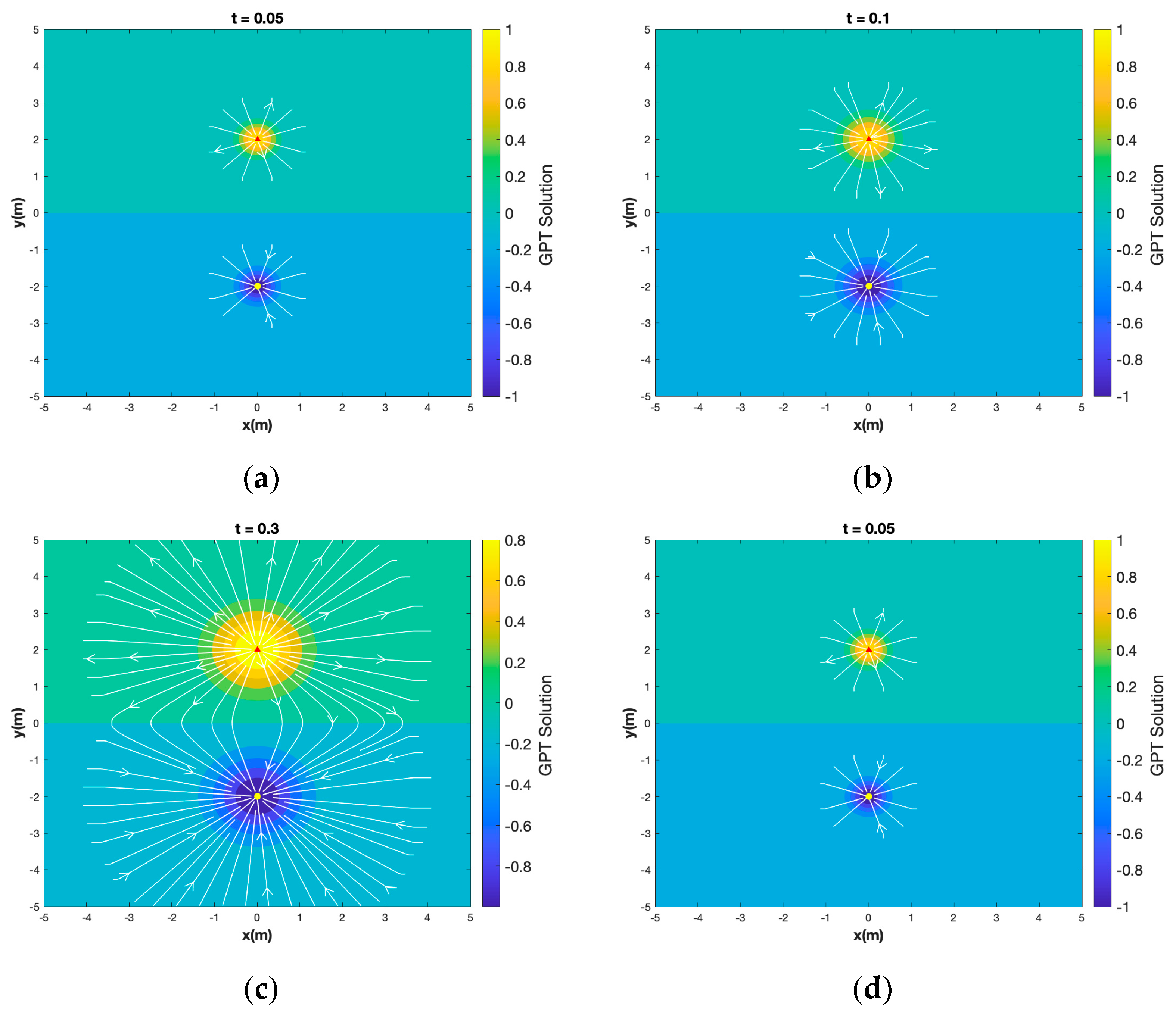
  • Case 2: Reservoir injected through a single vertical well
The Gaussian pressure transient solution is plotted in Figure 7 for a variety of times since the introduction of the pressure perturbation at the bottom of an injection well. The maximum pressure may not exceed the bottomhole pressure, which will raise the reservoir pressure in an asymptotic process and, in an infinitely large reservoir, not occur until time becomes indefinite.
Figure 8 shows the pressure saturation profiles at different times, initiated by a step change in pressure by one injector well located at the origin at x = 0 . Similar to the single producer case (Case 1), the pressure depletion curve converges to the horizontal y-axis of value y = PBH (the light blue line in Figure 8) for t = 1000 .
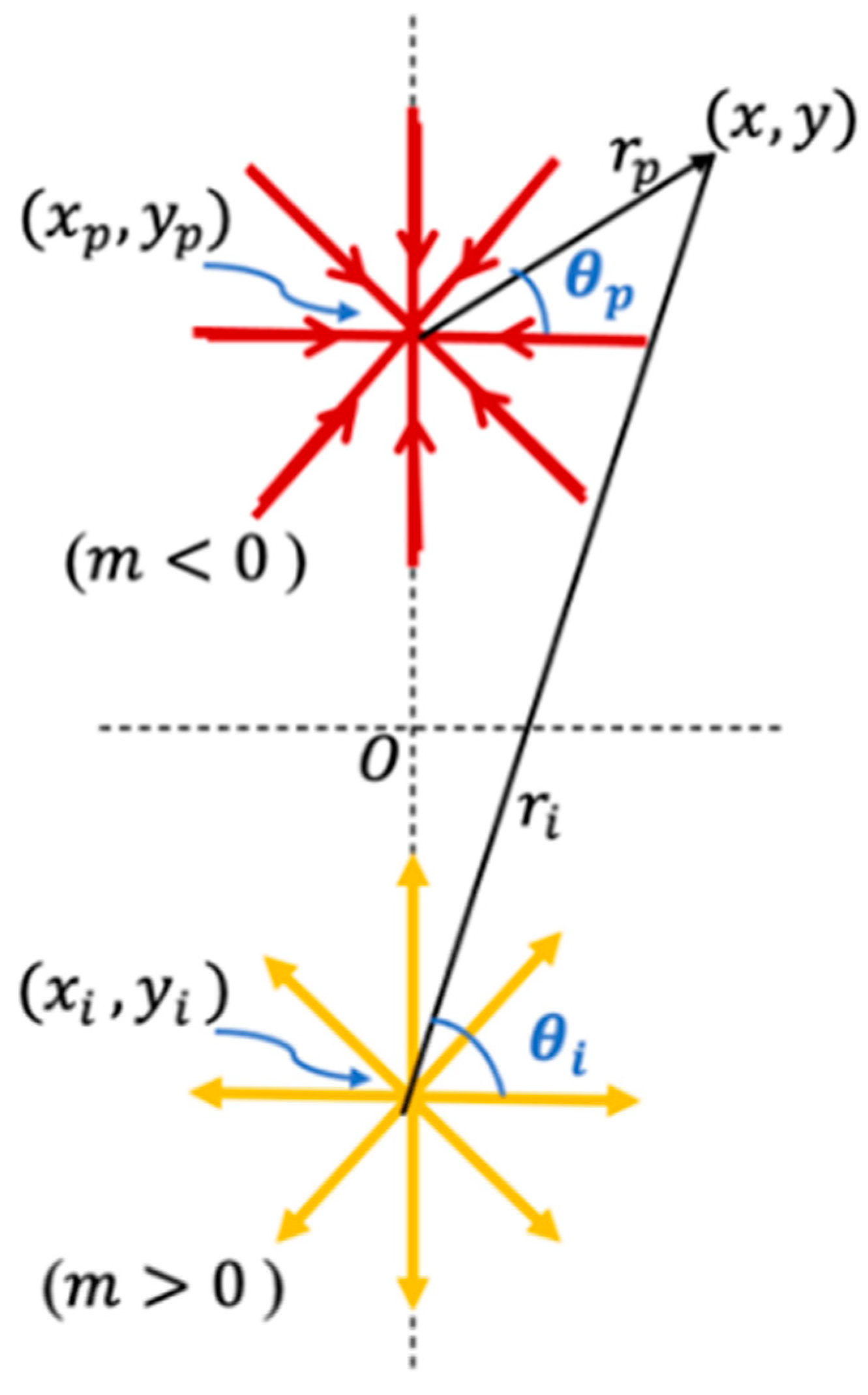
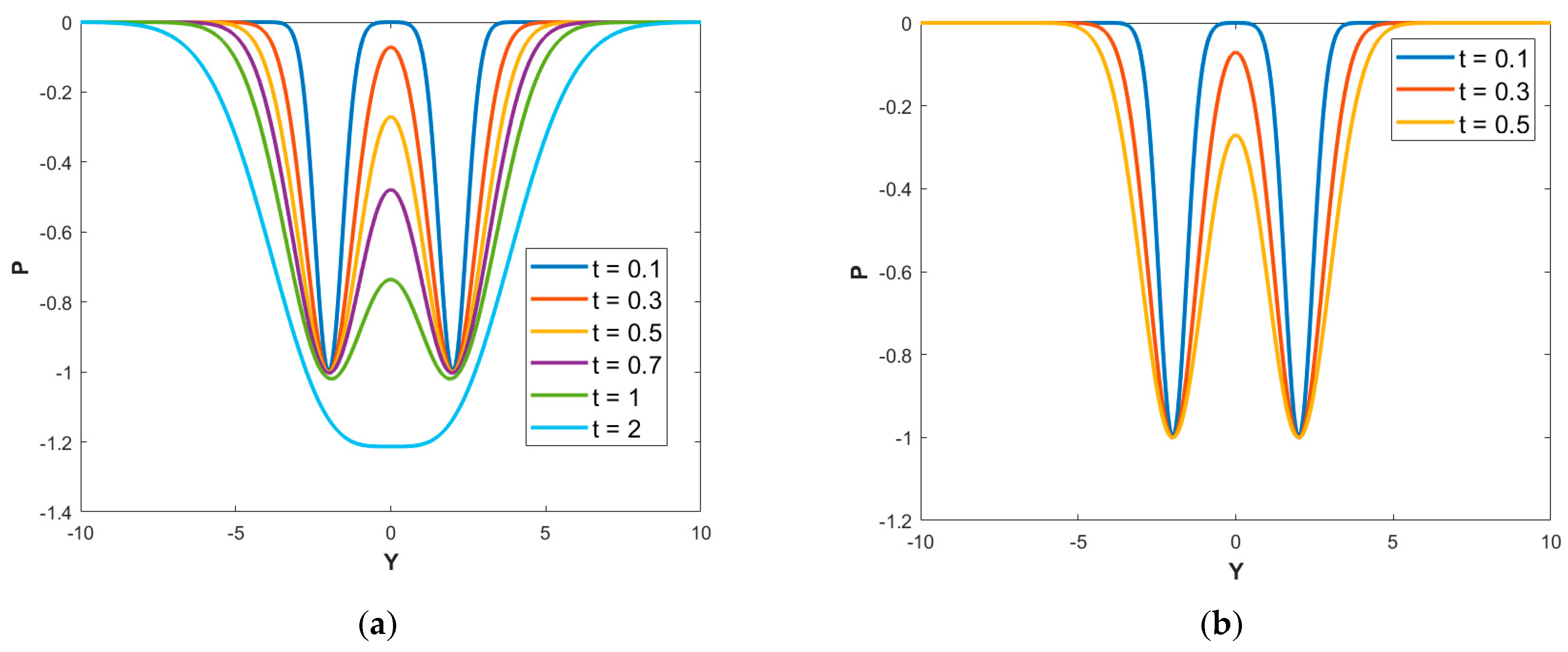
  • Case 3: Reservoir with a two-spot production system (one injector and one producer)
In case a reservoir has multiple sources of pressure change, say n vertical wells and/or n hydraulic fractures, with pre-existing reservoir pressure P 0 , the transient changes in the reservoir pressure (at any time t ), according to the classical superposition method, follow from the sum of Gaussian solutions for the pressure change due to each individual source in the system [16]:
P ( x , y , t ) = P 0 + k = 1 n Δ P ( x k , y k , t ) .
Consider a two-spot well constellation (Figure 4c), consisting of one producer located at ( x p , y p ) and one injector located at ( x i , y i ) , such that x p = x i and y p = y i . The classical 2D superposition Gaussian solution for the pressure change induced by the two wells (for the isotropic diffusivity case ( D x = D y = D h ) ) is given by:
Δ P ( x , y , t ) = Δ P 0 ,   i     e 1 4 t ( x i 2 + y i 2 D h ) + Δ P 0 ,   p   e 1 4 t ( x p 2 + y p 2 D h ) ,
where Δ P 0 ,   i   and Δ P 0 ,   p   are the bottomhole pressures for the injector well and producer well, respectively, assuming the pre-existing pressure in the reservoir is P 0 = 0 . If | Δ P 0 ,   i | = | Δ P 0 ,   p | , the system is called balanced doublet flow; otherwise, the system is called unbalanced doublet flow [24,25]. In [25], the authors used the somewhat un-English term unsymmetrical rather than asymmetrical. We are fine with both and prefer to use the dynamic term ‘unbalanced doublet’.
The pressure transient advance is graphed in Figure 9 for a balanced doublet. In this case, Δ P ( x , y , t ) may not drop below the bottomhole pressure of the producer well, i.e., Δ P ( x , y , t ) <  PBH, and a time limit stop, t l i m i t s t o p , is then triggered for the producer well; otherwise, the flow becomes non-physical. For the injector well, time t l i m i t s t o p occurs when Δ P ( x , y , t ) >  PBH; otherwise, the flow would become non-physical. The appearance of unphysical results at later times in the case of superposed pressure sources is briefly discussed in Section 5.2.
For a doublet well pair, beyond time t l i m i t s t o p , Δ P ( x , y , t ) would start to shift the pressure peaks beyond the injector location and the pressure minima beyond the producer location, which would be non-physical. New work in our research group [26] has revealed that for the superposition of pressure transients, non-physical solutions occurring at later times can be effectively remedied by modifying the classical superposition Equation (16c). In Figure 9d, the production time will continue, but the pressure gradient in the reservoir region between the two wells will have reached a steady state and will remain so as long as the producers and injectors have balanced injection and production rates. In the case of an uneven rate quota, the system is either a net producer (Figure 10a) or a net injector (Figure 10b).
Figure 11a,b show the pressure transient profiles for different times near a producer located at ( 0 , 2 ) and an injector located at ( 0 ,   2 ) . Here, x is fixed at x = 0 and y [ 10 ,   10 ] . In Figure 10a, the P B H is 5 for the producer well and 1 for the injector well. In Figure 10b, the P B H is 1 for the producer well and 5 for the injector well.
For the balanced doublet, the flow between the two wells will eventually reach a steady state when the pressure profile is represented by a straight line joining the points ( 2 ,   1 ) and ( 2 , 1 ) , i.e., when the pressure profile has become stable and no longer transient—no change occurs with respect to time (Figure 11a). The flow in the region between the two wells (i.e., at y [ 2 ,   2 ] ), reaches that steady state at t l i m i t _ s t o p 0.5 . For t > t l i m i t _ s t o p , the max and/or min values of P ( x , y , t ) would start shifting beyond the original well locations, and the flow would become non-physical.
For the unbalanced doublets, the flow (in the region between the two wells) needs longer to reach the steady state than for the balanced doublet case. Figure 11b,c show that the pressure transient period stops at t l i m i t _ s t o p 0.7 when the flow reaches the steady state in the region between the wells.

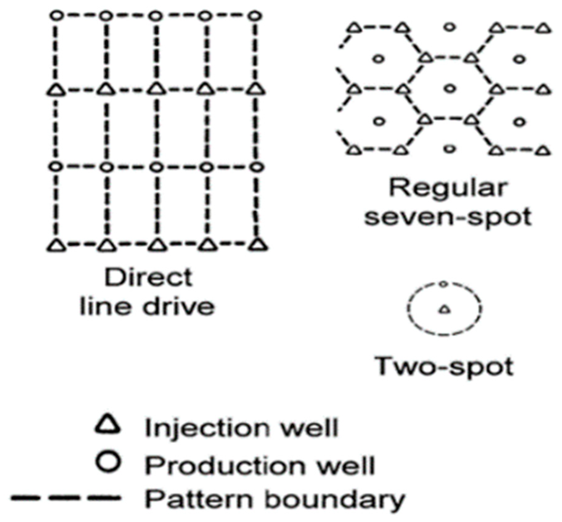
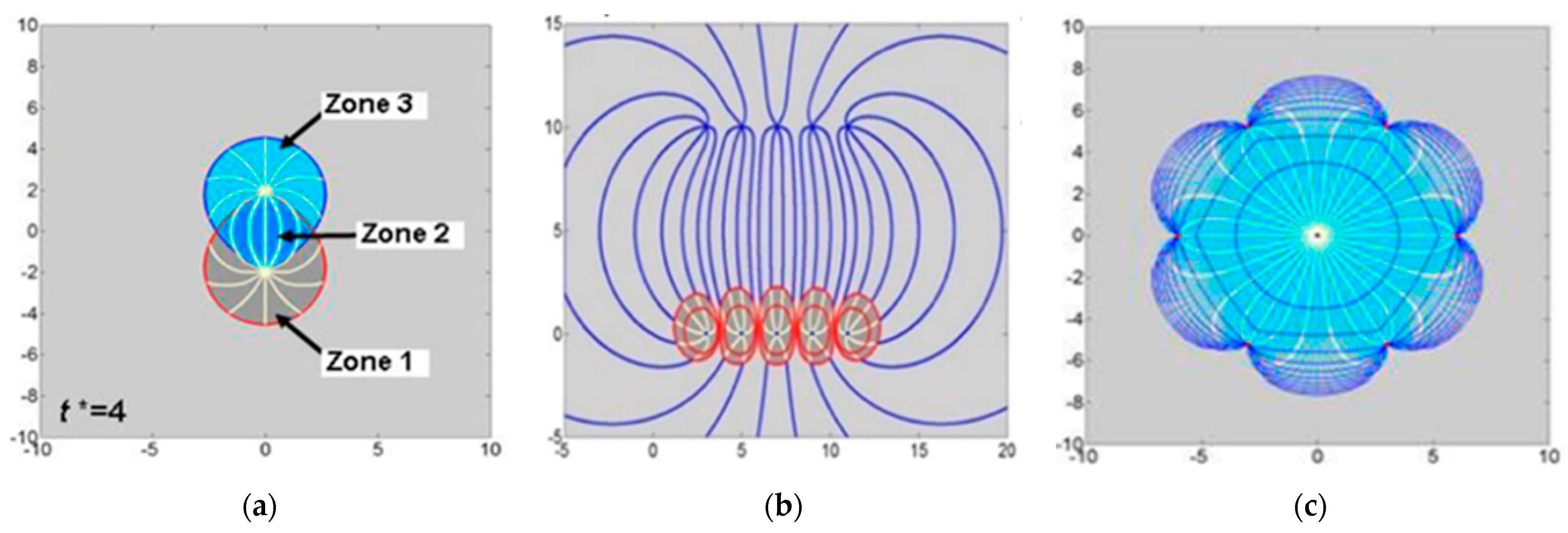
3. Fluid Flux and Flow Paths

In this section, we will use the fluid flux (see Equation (3b)) obtained from Darcy’s Law (in 2D) for isotropic and single-phase flow to plot the flow paths as the fluid moves from the porous reservoir rocks into the well system at any time before the flow reaches the steady state. We will use the Gaussian pressure transient (GPT) method to compute the pressure gradient P of Equation (3b). The fluid flux (Darcy velocity) q D   [ L T 1 ] in Equation (3b) is the flux from the porous formation into the open space of the wellbore across a unit area of wellbore exposed. Recall from Section 2.1 that the average fluid velocity ( u r ) in the porous reservoir is the Darcy velocity ( q D ) divided by the effective porosity ( ϕ ) of the medium, i.e.,
u r = q D ϕ = k ϕ μ P ,
which is similar to Equation (3a), but Equation (11) is for simplified cases with isotropic porosity and isotropic permeability (the off-diagonal elements in the tensor are zero and the diagonal elements are identical).
Based on the Darcy velocity components q D = ( q x ,   q y ) and pressure gradient components P = ( P x ,   P y ) , we can split Equation (3b) into two equations representing the Darcy velocity (m/s) in the x -direction and the y -direction, respectively:
q x = k μ P x ,
q y = k μ P y .
To plot the flow paths, we will consider some common, well-configured patterns that are either well-known or can be compared with published CAM solutions for steady state. CAM-based solutions are only capable of modeling steady-state flow patterns, while GPT-based solutions can model both the initial transient flow and the final steady-state. The comparison between GPT and CAM results must therefore be limited to the steady-state flow stages. Figure 12 shows typical steady-state flow path patterns in subsurface reservoirs (penetrated by two or more wells), as visualized in previous studies using the complex analysis method (CAM) [3,19,20,21,22].
  • Case 3: Doublet (two-spot well array)
The doublet flow pattern of Figure 12a corresponds to a balanced well pair as used in Case 3 of Section 2.4. In Figure 12a, the particle paths along the steady-state flow paths were traced with the CAM code using a Eulerian time-stepping schedule [19]. The front of the flow path is outlined by time-of-flight (TOF) contours. The blue outline in Figure 12a is for fluid advance of injected fluid, and the red TOF outline is for fluid withdrawal.
In the GPT solution of Figure 13a–d, the transient expansion of flow paths as the pressure advances in the reservoir space around the wells is mapped, together with the normalized pressure-change contours. The yellow dot marks the producer’s location, and the red triangle is for the injector. The injector and producer are spaced by four length units. The white flow paths are traced with MATLAB using P from Darcy’s Law. Note that the pressure-change contours everywhere are perpendicular to the flow paths (as expected in the absence of inertia).
An important feature of the GPT method is that it can visualize the flow during the earlier period of pressure transient advance in a reservoir before the steady-state flow is established. The advance of the pressure gradient into the reservoir space is shown in Figure 13a–d, together with the instantaneous flow paths. Note that before the pressure transient fronts of the respective wells meet, the flow paths of the injector and producer wells are perfectly radial (Figure 13a,b). After pressure interference starts occurring, the shape of the pressure contours is no longer concentric (Figure 13c,d), and flow paths begin to attain the well-known steady-state pattern of a doublet flow. Any major deviation from the doublet flow patterns at steady-state is due to the use of the classical superposition method (cf. Equation (10a)), as will be confirmed in forthcoming work by our group.
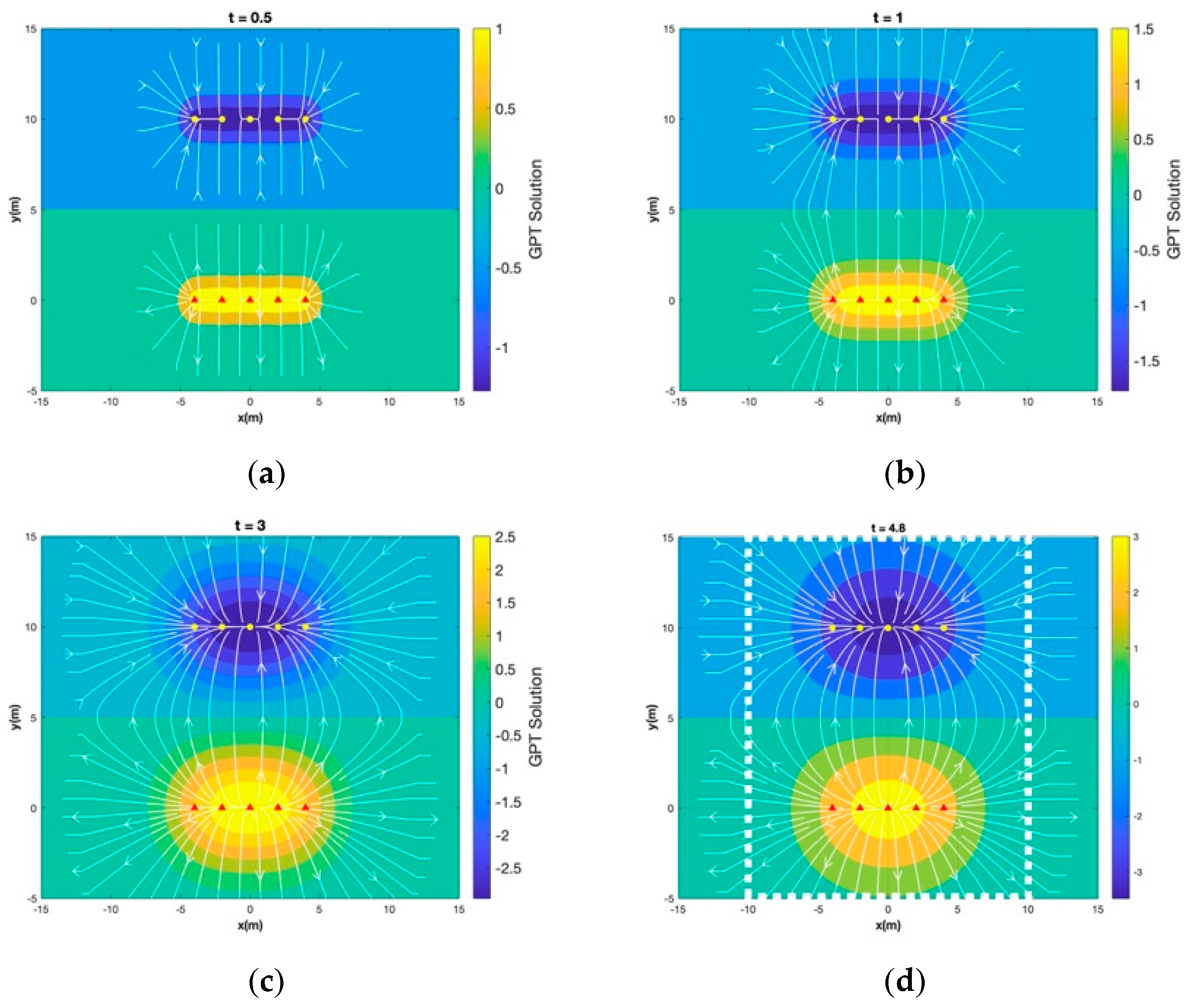
  • Case 4: Direct line drive (five-spot well array)
The direct line drive of Figure 12b assumes a balanced well array in direct line drive arrangement (Figure 1), with 5 injectors placed on y = 0 and 5 producers placed on y = 10 . The GPT solution method was used to generate the transient Gaussian pressure profiles (colored contours) and flow paths (white lines) for the same well constellation (Figure 14a–d). Initially, the flow patterns of the lower injectors (red triangles) and upper producer row (yellow circles) are not connected and will lead to pressure profile development similar to that portrayed in Figure 13a for the balanced doublet. Once the pressure fronts of the injectors and the producers meet, a steady-state pressure profile is established in the space between them (Figure 14d). The flow of the direct line drive well array will resemble that of the steady-state doublet (Figure 12b).
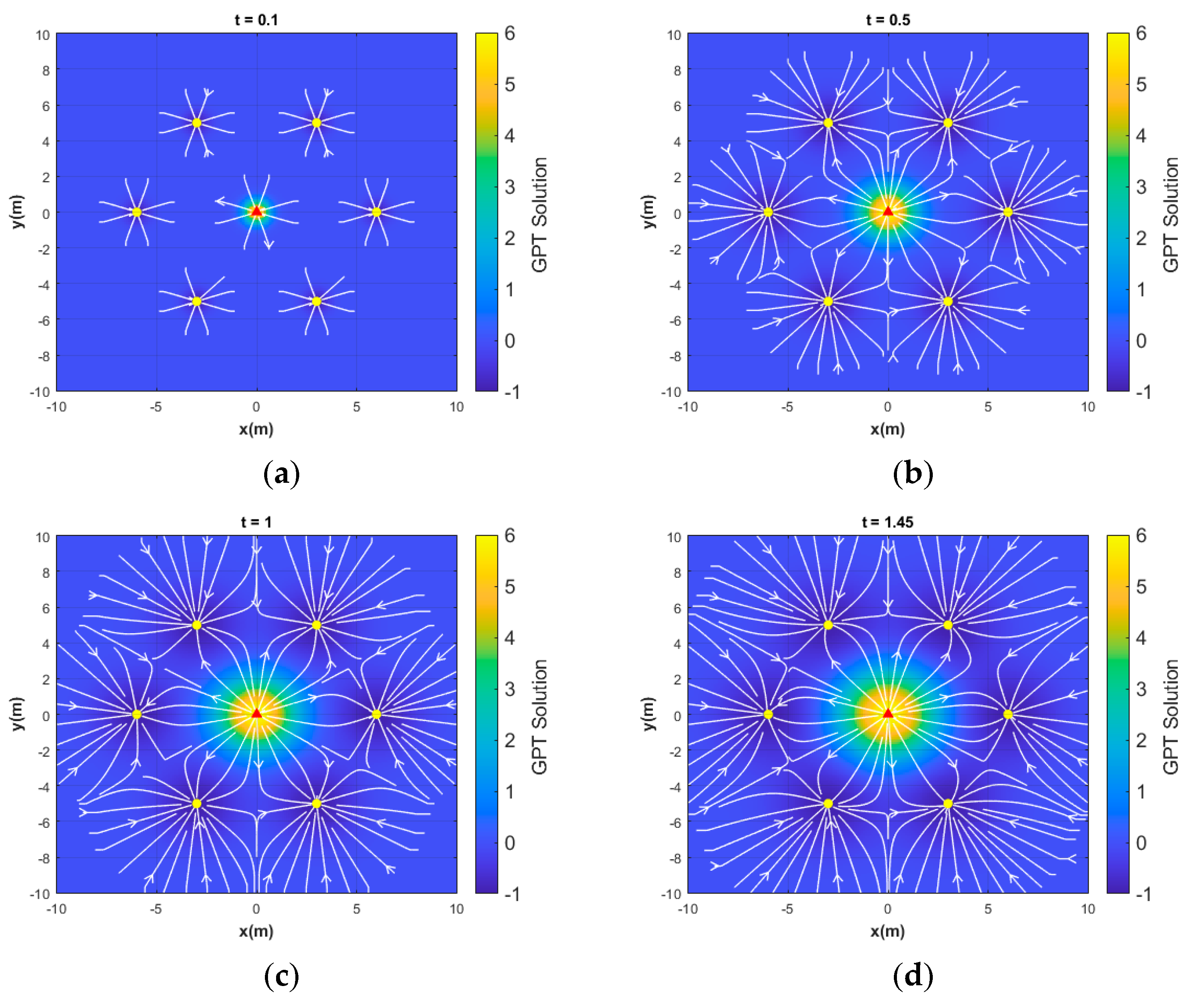
  • Case 5: Seven-spot well pattern
The 7-spot well pattern of Figure 12c had one strong injector in the center and six producers spaced equally around the central injector well. The injection rate of the single injector was equal to that of the six producers combined. The same well strengths were used in the realization of the GPT flow paths in Figure 15a–d, with one strong injector (red triangle) in the center, surrounded by six producers (6 yellow circles). The advance of the pressure change contours is shown, and the flow is evenly fanning radially outward from the central injector and toward the six surrounding producers at an early time before the flows approach each other (Figure 15a).
Once the pressure gradient is extended in the circular region around the central injector well, the flow paths are no longer radial (Figure 15b–d). The final stage (Figure 15d) occurs when the flow pattern becomes steady-state, similar to that seen in Figure 12c. However, it is worth noting again that the solution in Figure 12c was produced with the CAM using a time-stepped superposition method while tracking the advance of certain fluid tracer particles starting from the injector wells as they move toward the producer wells. However, this procedure is the CAM and is constrained by the superposition of steady-state solutions. In contrast, the GPT solutions of Figure 15a–d show the evolution starting from transient flow, while the pressure transient advances to ultimately establish steady-state flow.

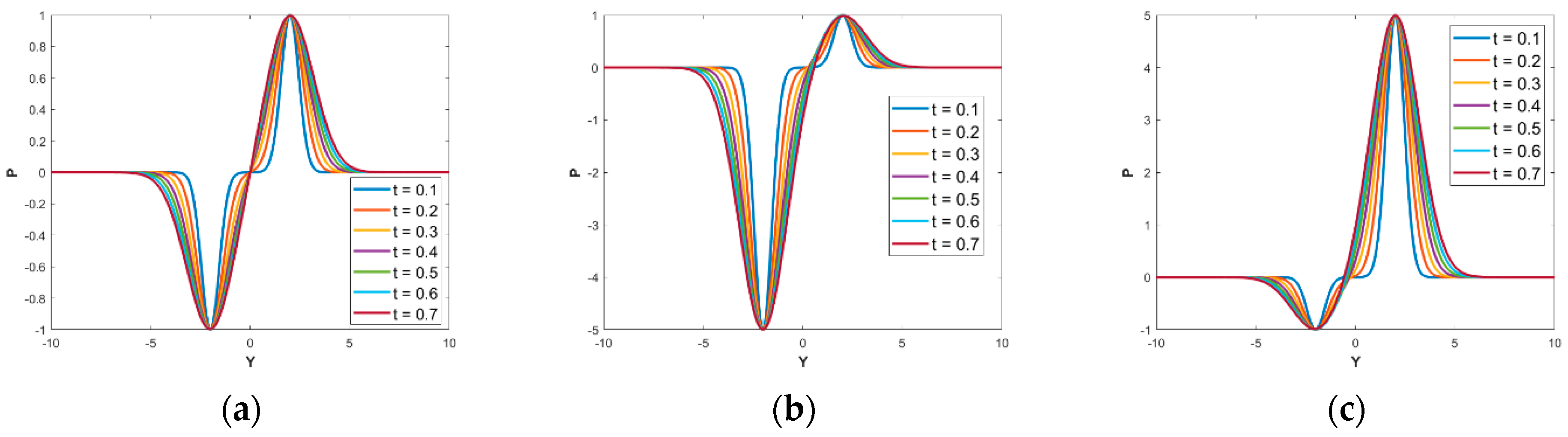
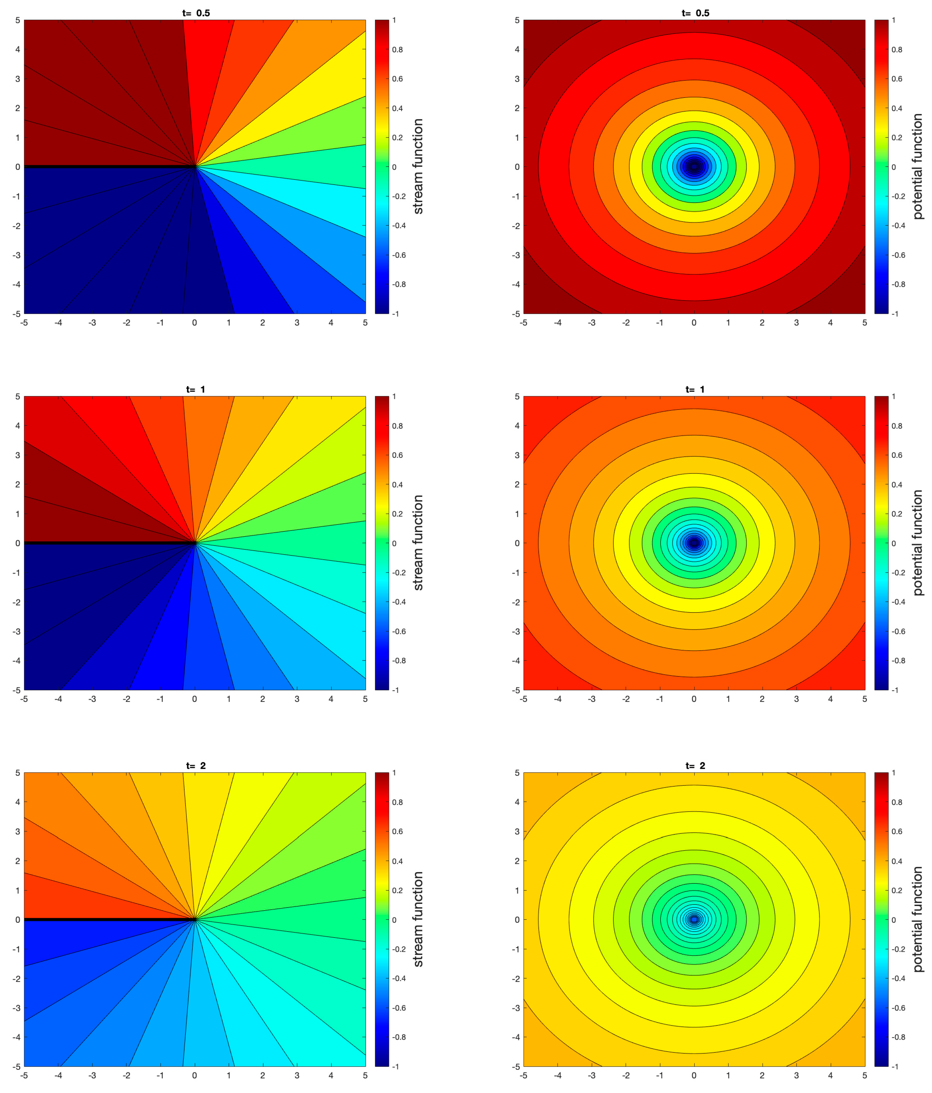
4. Derivation of the Transient Stream Function and the Transient Potential Function

In Section 3, transient solutions for flow paths and pressure contours were computed based on gridded solution points solved after computing P using MATLAB (see Appendix B). However, true analytical GPT solutions can be obtained by deriving the stream function and potential function for transient flows. The essential fundamentals are given (Section 4.1), before applying those to the GPT solution to derive the new analytical stream function and potential function solutions for transient flow (Section 4.2 and onward).

4.1. Fundamentals

The transient GPT solutions of the temporal and spatial pressure changes [16,17,18] can be used to compute the potential function and stream function of the time-dependent fluid flow. The fluid flow in our study is subject to an incompressibility assumption. However, the flow does not need to be inviscous (see arguments in Weijermars [20]). The flow can be described by combining the stream function ψ ( x ,   y , t ) and velocity potential function φ ( x ,   y , t ) to satisfy the Cauchy-Riemann equations [20]:
φ x = ψ y ,                               φ y = ψ x   .    
The stream function is a scalar function that can be solved for constant values to plot the streamlines; its spatial derivatives give the fluid velocity components, u x and u y [20,27,28]:
u x = ψ y ,    
  u y = ψ x .  
Consider a reservoir with a single source or sink located at the origin (Figure 16). The GPT solution of a single source or sink is given by Equation (10a) for n = 1 with Δ P < 0 for sink flow (producer well case) and Δ P > 0   for source flow (injector well case). Typically, to obtain the stream function, one can integrate Equation (14a) with respect to y and Equation (14b) with respect to x (see, for example, Weijermars [26]). However, to avoid the complexity of integrating the exponential function in Cartesian coordinates (which appears in the velocity components by differentiating the transient pressure), one can, alternatively, consider the radial and tangential velocity components ( u r a d , u θ ) of the source or sink flow given by (see [27]):
u r a d = m 2 π r ,                     u θ = 0 ,
where m is a scaling space constant that represents the strength (volumetric flow rate per unit length in m2/s). If m is positive, the fluid is flowing radially outward from the origin (source flow), and if m is negative, the fluid is flowing radially toward the origin (sink flow) (see Figure 16). To solve and find the well strength, m, we use the stream function and velocity potential for the source or sink flow obtained from integrating u r a d in Equation (15) with respect to r and integrating u r a d with respect to θ to get (see [27] for derivation):
ψ ( r , θ ) = m 2 π θ ,            
  φ ( r ,   θ ) = m 2 π ln r .
Having obtained the stream and potential functions of Equation (16a,b), one may revert to Cartesian coordinates if needed, using transformation from polar coordinates:
r = x 2 + y 2 ,           θ = tan 1 ( y x ) ,
Substituting Equation (17) in Equation (16a,b) gives:
ψ ( x , y ) = m   tan 1 ( y x ) ,
φ ( x , y ) = m 2 π ln x 2 + y 2 ,
The fundamental set of fluid dynamic principles and equations of Section 4.1 will be used in Section 4.2 to derive the stream function and potential function solutions. The goal now is to compute the strength m based on the pre-computed transient pressure using GPT solutions.

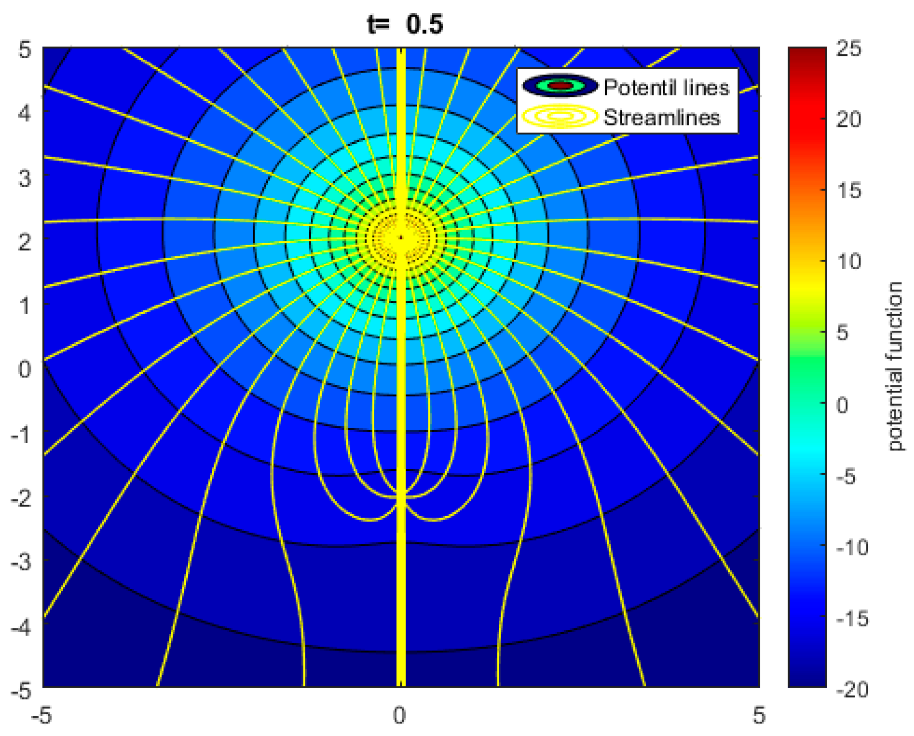
4.2. Transient GPT Stream Function and Potential Function

The well-strength m in Equation (18a,b) for a vertical well draining over its full length a reservoir of finite thickness h is given by m = q w / h , where q w is the volumetric flow rate as given in Equation (3c). Substituting the gradient of the GPT solution in Equation (3c), the volumetric production rate of a well with radius   r is given by:
q w ( t ) = h κ π r 2   μ β t   D h     Δ P 0   e r 2 4 t   D h .
Figure 17 shows the reduction in the production rate over time for a vertical producer well located at the origin with a radius of   r = 1 .
As shown by Figure 17, the flow rate is initially increasing when 0 < t < 1 , but after   t = 1 , it decreases rapidly and continues decreasing until it becomes a constant close to 0 for a very long time. The transient flow behavior of the flow rate, for both the sink and source flows, is consistent with our previous discussion in Section 2.3, where we concluded that for a reservoir with a single well (Case 1 for producer and Case 2 for injector), no steady-state flow will ever be reached.

4.3. Plotting Transient Stream Function and Potential Function

Next, we will use the flow rate q w ( t ) in Equation (19) to visualize the streamlines and potential lines during the transient flow period. An important feature of the GPT solution is that the transient stream function and potential function can be solved at any time after the onset of flow. In Figure 18, we plot the streamlines and potential lines for a source flow using the input values shown in Table 1.
The first column of Figure 18 shows streamline visualization (the straight radial lines in rainbow colors) with simple contouring for the stream function given by Equation (18a). The second column shows the equipotential lines as concentric circles in rainbow colors around the source position.

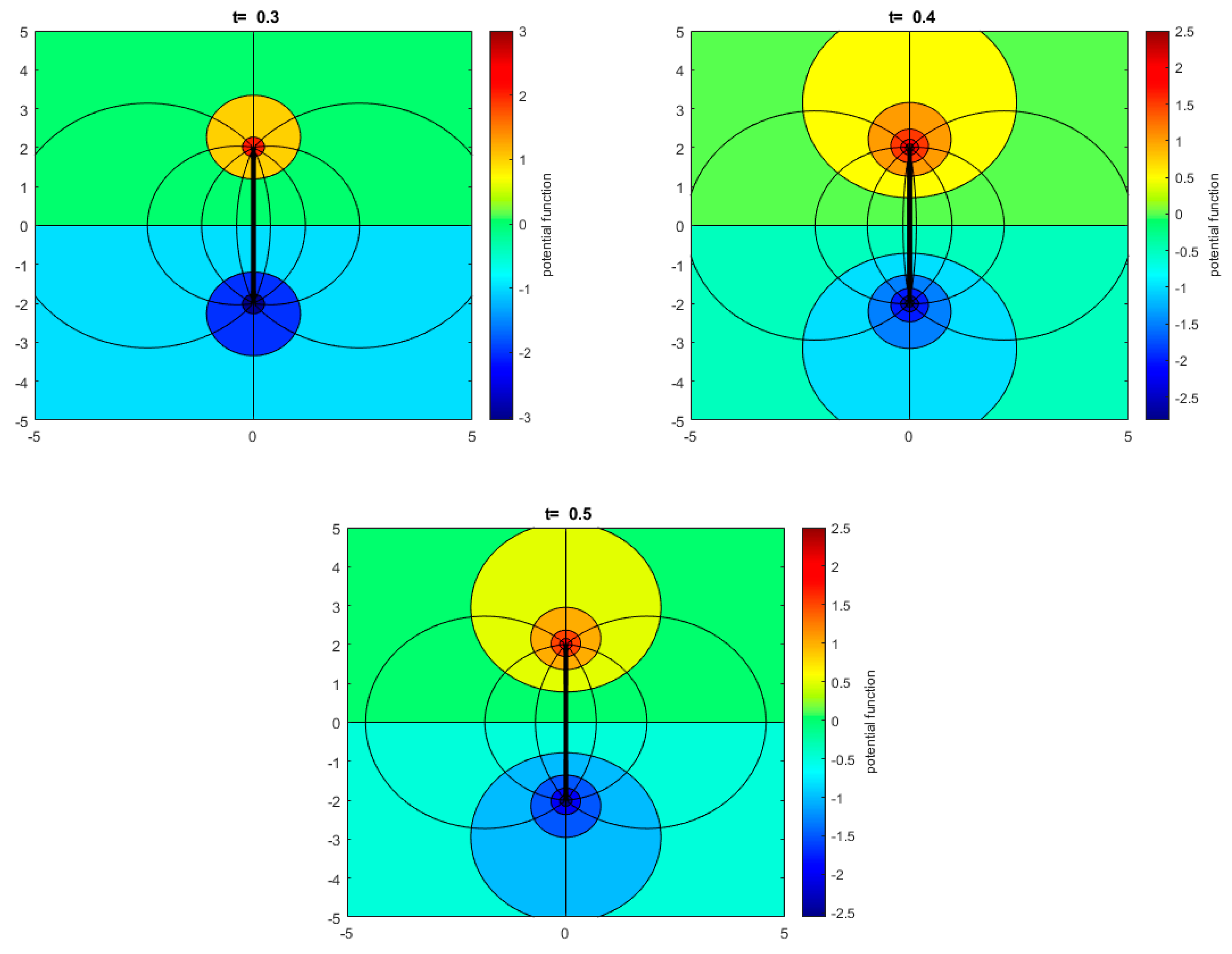
4.4. Transient Stream and Potential Functions for Balanced Doublets

Consider a reservoir with a source (injector) located at ( x i ,   y i ) and a sink (producer) located at ( x p ,   y p ) , such that x p = x i and y p = y i , as illustrated in Figure 19. Assume that | Δ P 0 | for the injector well equals | Δ P 0 | for the producer well (balanced doublet flow).
Before the pressure fields meet, due to the source flow and sink flow (Figure 13a,b), the stream function and potential function for each individual flow are as given by Equation (18a,b) for the single source and sink flows. However, as the pressure fields meet (Figure 13c,d), the well pair obeys a combined stream function [Equation (20a)] and potential function [Equation (20b)] (see [27]):
ψ ( r , θ ) = m 2 π ( θ i θ p ) ,                                                                      
φ ( r , θ ) = m 2 π ( ln r i ln r p ) = m 2 π ( ln r i r p )   ,
where θ p ,   θ i ,   r p , and r i are as shown in Figure 19.
Converting Equation (20a,b) into Cartesian coordinates gives the following equations:
ψ ( x , y ) = m 2 π ( tan 1 y y i x x i tan 1 y y p x x p ) ,
φ ( x , y ) = m 4 π   ln ( x x i ) 2 + ( y y i ) 2 ( x x p ) 2 + ( y y p ) 2   .                    
For the balanced doublet, the injection rate equals the production rate in magnitude, and both are obtained using Equation (19). Therefore, the well strength in Equation (21a,b) is computed by dividing Equation (19) by the thickness h of the reservoir.
The analytical solutions of the stream and potential functions of the balanced doublet flow are shown in Figure 20 using the input parameters in Table 2. The streamlines (black contours) and potential lines (colored contours) are plotted after the doublet flow has been established at times t = 0.3 ,   0.4 and 0.5 (the t s t o p l i m i t , see Section 2.4, Case 3). The streamlines for the sink flow and source flow are identical (as in Figure 18) before the pressure change fronts of the two wells reach each other. After the pressure transients meet, the streamlines start to curve up (for source flow) and down (for sink flow), establishing the typical steady-state doublet flow patterns (Figure 20). In our simulation, the moment when the two flows meet is considered to be at the time when there is a non-zero pressure gradient midway between the two wells on the line where their respective pressure transients meet (x-axis in our case), at which stage there comes into existence a flow across this line for the first time, passing fluids to the other side of the half space initially occupied by the fluid.

4.5. Transient Stream and Potential Functions for Unbalanced Doublets

For unbalanced doublets, consider a reservoir with a source (injector) located at ( x i ,   y i ) with source strength m > 0 and a sink (producer) located at ( x p ,   y p ) with sink strength α m for some positive integer α . The results of a well pair with an unbalanced net rate will develop asymmetrical (or unsymmetrical [24,25]) flow patterns.
The stream and potential functions for an unbalanced doublet flow in Cartesian coordinates are given by the following equations:
ψ ( x , y ) = m 2 π ( tan 1 y y i x x i α tan 1 y y p x x p ) ,                                                                                                                
φ ( x , y ) = m 4 π   [ ln ( ( x x i ) 2 + ( y y i ) 2 ) α   ln ( ( x x p ) 2 + ( y y p ) 2 )   ] .
Using the input parameters as in Table 3, we plot the analytical solutions for stream and potential functions for an unbalanced doublet flow in Figure 21, when the sink strength is 5 times the source strength ( α = 5 ). Since the sink strength is larger (in magnitude) than the source strength, the sink flow is dominant. An identical flow path for an unbalanced doublet was modeled in a previous study using CAM simulations [3].

5. Discussion

The extraction of natural resources (e.g., water, oil, gas, and geothermal fluids) is made possible by engineering interventions (such as drilling vertical or horizontal wells) that cause pressure changes in the reservoir space hosting these resources. Such pressure changes can be quantified using Gaussian pressure transients and then translated to visualize the relevant flow attributes (such as flow paths and well rates) at different times. The time dependency of the GPT solution can be used to compute the spatial pressure changes in the reservoir at any time, in response to an initial, instantaneous change in the bottomhole pressure ( P B H ), which occurs when the wells in the production and/or injection modes are switched on. For example, the evolution of the transient pressure profiles for a single producer when the (dimensionless) bottomhole pressure is equal to 0.5 is shown in Figure 22a. If we let an instantaneous change in the bottomhole pressure occur at and after time t = 10   (the P B H  changed from 0.5 to  1 ), we can see that the transient pressure profile has an instantaneous response to the change in the bottomhole pressure, as shown in Figure 22b.

5.1. Novelty of GPT Solutions for Stream and Potential Functions

The visualization of fluid flow in porous media is commonly based on numerical and semi-analytical methods that require space and time discretization. For time-dependent, or so-called transient flow problems, tracing the rapidly changing flow paths is an additional challenge. The GPT solution was used in this study to analytically solve the potential and stream functions during the transient flow period. Such transient solutions for well problems have not been presented before, in spite of the long-standing history of solving the steady potential and stream functions.
In the present study, we presented analytical solutions for the stream function, which can compute both the steady-state and the transient flow paths around wells draining fluid from porous media. Likewise, potential function solutions are derived by computing the pressure gradients for both the steady-state and the transient flow stages. Our new solutions for the stream and potential functions are based on analytical computations of the Gaussian pressure transients (GPT) [16,17]. Using GPT solutions, one can visualize the flow paths at any time during the transient flow period (see Section 3). Here, the transient flow period refers to the period when there is an advancing pressure gradient, causing the transient flow paths to shift over time.

5.2. Superposition of Pressure Transients

The computation of the interaction of the pressure transients of multiple wells has also led to fundamental insights about certain superposition effects that require further investigation. Several non-physical aspects came to light when superposing pressure transients using the traditional superposition Equation (10a):
(1)
When we arrest the pressure transient advance between a pair of producer wells to avoid the pressure dropping below the bottomhole pressure, as in Figure 23a, the far-field pressure advance is also frozen (Figure 23b). This can be overridden by continuing the advance of the pressure front in the far-field region, but this leads to an outer region with the time counter increasing, while in the inner region the time has already stopped (at t l i m i t _ s t o p ) when the bottomhole pressure is reached.
(2)
For an injector and producer well pair, t l i m i t _ s t o p is introduced when the pressure profile between the wells has been established (Figure 11a). However, here the far-field pressure advance is also frozen, and the far-field pressure front would no longer advance in the far-field when the pressure profile in the inner region between the doublets has been established (a pseudo-steady state).
This paradoxical conclusion of the t l i m i t _ s t o p is a result of using a classical superposition method according to Equation (10a). To avoid the non-physical effects of conflicting time counters in the inner regions and the far-field flow regions, a modified superposition method has been developed, which mitigates this issue (work under review).

6. Conclusions

A method is presented for modeling fluid flow in porous media using new solutions of the pressure diffusion equation based on Gaussian pressure transients (GPT). Fluid flow can be visualized for both the transient and steady-state stages by computing the local pressure gradient analytically. The ability to visualize the transient flow stage is important because it provides information about the flow paths that could help optimize well placement and design when extracting natural resources from subsurface reservoirs. The Gaussian solution method is free of the computational complexity of time-stepping. GPT solutions therefore provide a fast alternative to numerical solution methods, which are relatively complex to use and have long computation times, especially for sensitivity studies and well-placement optimization. The faster and less complex computations make the GPT method an attractive option for optimizing natural resource extraction strategies.
Examples are given of how to use Gaussian solutions of the diffusion equation to visualize fluid flow paths in subsurface reservoirs as required for the extraction of natural resources such as oil, gas, water, and geothermal fluids. The Gaussian method is extended in our study by computing and visualizing velocity magnitude contours, streamlines, and other flow attributes in the vicinity of well systems that deplete pressure in a reservoir. The GPT method uses the Gaussian probability function of Equation (9), which then gives the spatial and temporal characteristics of the pressure change in 1D, 2D, and 3D (Equations (7) and (8a,b)). The GPT solution form is a simple expression that provides a fast analytical method to compute flow patterns with high resolution.
To validate the performance of the GPT method for computing the flow paths due to transient pressure changes in superposed well systems, we compared the GPT solutions with those previously obtained using an independent closed-form solution based on the complex analysis method (CAM), assuming the same initial conditions. The comparison shows a good match for the steady-state flow patterns (see Section 3). The CAM can only visualize steady-state flow paths. However, GPT solutions allow us to visualize the solutions of the stream and potential functions for both the steady-state and transient stages of the flow development, again without the computational complexity of time-stepping.
The transient pressure changes in the superposed well system can be rapidly computed by superimposing GPT solutions for the pressure transients due to individual well and/or fracture sources of pressure change in the system. Using the standard equations to compute the pressure derivatives, we visualized the flow paths in the reservoir during the pressure transient period. The GPT method can predict well productivity and injectivity based on the applied bottomhole pressure and the applicable hydraulic difusivity of the reservoir system and then help trace the fluid migration paths in the reservoir. The solutions presented are applicable to both fluid production and fluid injection cases, such as those used for the disposal or storage of waste fluids, carbon dioxide, hydrogen, and natural gas.
The main points of the paper are:
  • Gaussian solutions of the diffusion equation can be used to visualize flow paths during transient pressure changes in subsurface reservoirs due to pressure gradients caused by engineering interventions.
  • The Gaussian method was extended to compute and visualize velocity magnitude contours, streamlines, and other flow attributes in the vicinity of well systems that are depleting pressure in a reservoir.
  • Stream function and potential function solutions were derived for instantaneous modeling of flow paths and pressure contour solutions of transient flows without time-stepping.
  • The GPT method can compute the local pressure gradient analytically based on Gaussian pressure transients to model fluid flow and compute the fluid flux from the reservoir into the well system.
  • The GPT method can predict fluid extraction rates and study the fluid origin in reservoirs; the method can also model fluid injection in subsurface reservoirs when used for the disposal or storage of certain fluids.
  • The computational efficiency of the analytical GPT solution method compares favorably to numerical methods for sensitivity studies and well-placement optimization.

Author Contributions

Software, S.A.; Validation, M.A. and R.W.; Investigation, M.A. and S.A.; Supervision, M.A. and R.W.; Project administration, R.W. All authors have read and agreed to the published version of the manuscript.

Funding

This research received no external funding.

Acknowledgments

The authors acknowledge the generous support provided by the College of Petroleum Engineering & Geosciences (CPG) and department of mathematics at King Fahd University of Petroleum & Minerals (KFUPM).

Conflicts of Interest
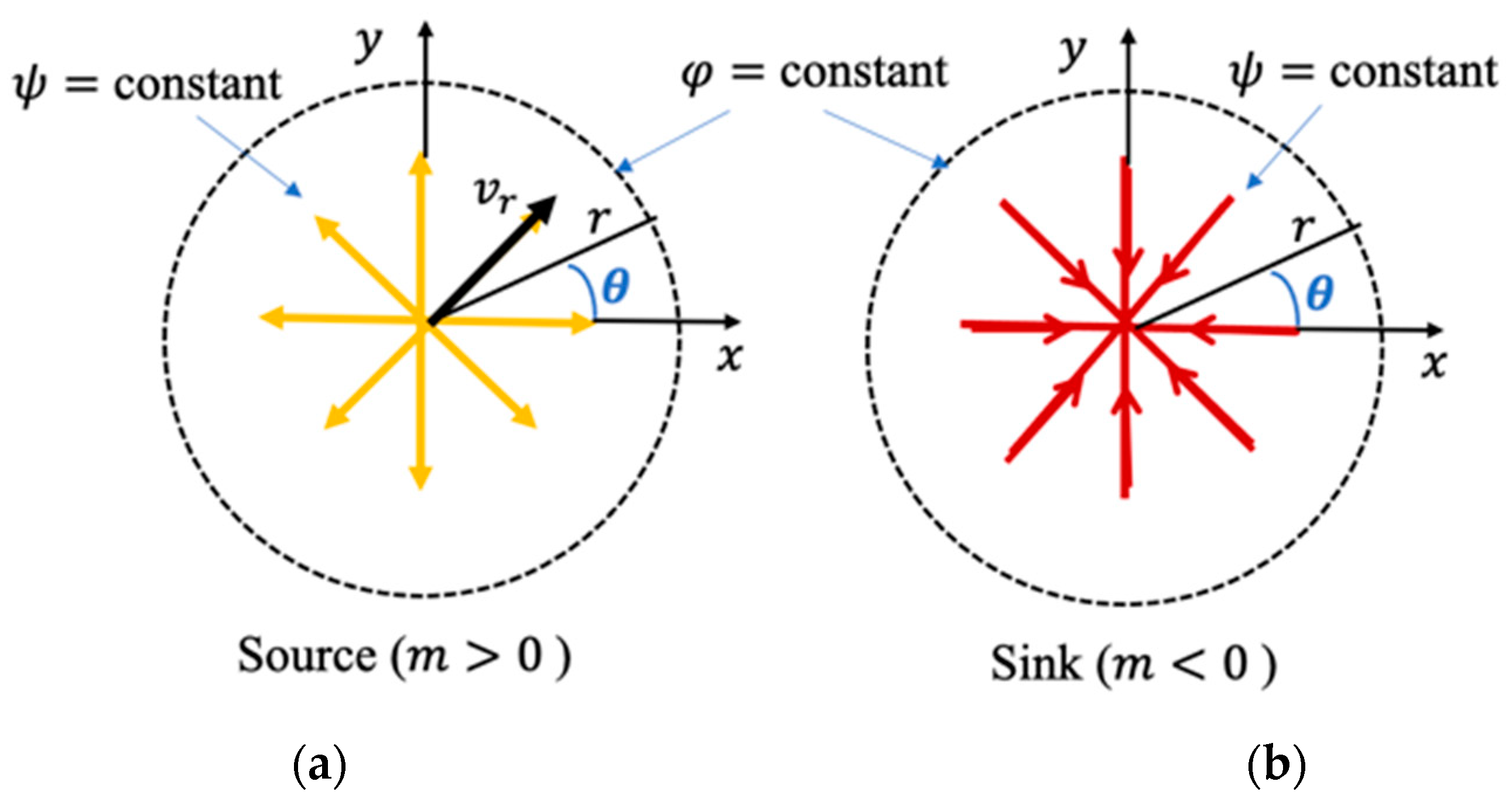
The authors declare no conflict of interest.

Nomenclatures

u Fluid velocity μ Fluid viscosity
u r Fluid velocity in porous medium κ Permeability
u x Velocity component in x -direction ϕ Porosity
u y Velocity component in y -direction ρ Fluid density
u r a d Radial velocity β Formation volume factor
u θ Tangential Velocity r w Wellbore radius
q D Fluid flux (also called Darcy velocity) h Reservoir thickness
q x Darcy velocity in x -direction p Gaussian probability-function
q y Darcy velocity in y -direction W f Half-length of a hydraulic fracture
q w Volumetric rate D h Hydraulic diffusivity
P Pressure D x Diffusivity in x -direction
Δ P Pressure change D y Diffusivity in y -direction
Δ P 0 Local pressure change m Well strength (volumetric flow rate per unit length)
P 0 Initial reservoir pressure ψ Stream function
P B H Bottomhole pressure φ Potential function

Appendix A. Dimensional Scaling of Physical Quantities

Dimensional analysis is a technique to transform an equation featuring physical quantities of certain units into non-dimensional form (see [28]). For example, consider the dimensional Gaussian Equation (7a) for the advance of a 1D diffusion along the x-axis front from a planar source in the origin:
Δ P ( x , t ) = ( P 0 P B H )   e x 2 4 D h t
This dimensional equation (with dimensional units) can be converted into a non-dimensional equation (with non-dimensional units) by dividing the variables by a typical unit with the corresponding dimension. For example, for the case of Equation (A1), one should use dimensional unit measures for the fundamental physical quantities, such as length ( x 0 = 1   m ) and time ( t 0 = 1   s ), for the divisions of the corresponding dimensions x and t   to obtain the non-dimensional units x * and t * :
x * = x x 0       t * = t t 0
The remaining parameters in Equation (A1), D h   and   P , are so-called derived quantities, with their dimensions being determined by certain fundamental quantities, as in Table A1.
Table A1. Dimensional analysis.
Parameter Description Dimension
x ,   x 0 Length; characteristic length unit [L]
t ,   t 0 Time; characteristic time unit[T]
D h Hydraulic diffusivity[L2T−1]
P Pressure[ML−1T−2]
The hydraulic diffusivity, D h , can now be non-dimensionalized as follows:
D h * = t 0 D h x 0 2
Likewise, one may non-dimensionalize the pressure, P , by multiplying with the inverse of its fundamental units:
P * = P x 0 t 0 2 m 0
However, because mass, m , does not feature as a separate fundamental quantity in Equation (A1), using the typical unit mass, m 0 , is not very practical for non-dimensionalizing P . Instead, we may use an alternative approach and simply normalize the term ( P B H P o )   by the initial reservoir pressure, P 0 . Substituting all the proposed normalizations, the non-dimensional form of Equation (A1) becomes:
Δ P * ( x * , t * ) = ( P 0 P B H P 0 )   e ( ( x * x 0 ) 2 4     D h * x 0 2 t 0   t * t 0 )     = ( 1 P B H P 0 )   e ( x * 2 4   D h * t * )
The principal purpose of the scaling procedure is to subsequently be able to work with non-dimensional units for x * , t * , and   D h * , and corresponding dimensional quantities x , t , and D h can be computed anytime using Equations (A2) and (A3). For example, a non-dimensional diffusion travel distance of x * = 10 over a non-dimensional time of t * = 105, when working in dimensional SI units with x 0 = 1   m and t 0 = 1   s, will correspond to dimensional quantities of x = 10   m and t = 10 6   s. When we do experimental runs, we can simply start from t * = 0 and evaluate for a certain spatial domain bound by x M A X * , how Δ P * ( x * , t * ) changes over a distance of 0 x * x M A X * . Of course, for a 2D diffusion process using the point sources in our study, we also have 0 y * y M A X * .   The values of x M A X * and y M A X * depend on where the front of the pressure transient is studied for a given D h * .
For each set of model runs, D h * will normally not change but is chosen as a typical value for the system studied. For example, in reservoir rocks, the dimensional values of the hydraulic diffusivity in geological reservoirs may range from 10 2   m 2 s 1 for coarse sandstone formations (with high permeability) to 10 10   m 2 s 1   for very tight shale formations (with ultra-low permeability). If we chose for our models an average dimensional value of D h = 10 6   m 2 s 1 , the corresponding D h *   will be 10 6 .
If instead of using D h * = 10 6 , we use an arbitrary value of D h * = 1 , that means we are modeling a physical porous medium with diffusion rates much faster than those that occur in oil and gas reservoirs. Such models of D h * = 1   are still useful but will have very short runtimes ( t * on the order of 10 n ) to cover the diffusion distances that in geological reservoirs would require much longer times ( t * on the order of 10 n ).
Finally, if we work with non-dimensional velocities (as in Section 4), these can be normalized using x 0 and t 0 because velocity has the dimensions of [LT−1].

Appendix B. Coding Hints

The results visualized in our study were generated by coding (in MATLAB) the principal analytical equations presented in our study, following a workflow schedule as detailed in Figure A1.
First step: define all the inputs of the model to be solved
  • The computational domain [ a , b ] (example, a = −5; b = 5),
  • Number of mesh points in each direction (example, N = 10),
  • The bottom hole pressure for injector(s) and/or producer(s),
  • Well positions for injectors and/or producers (example, x_inj = 0; y_inj = 2; x_prod = 0; y_prod = −2),
  • Time variable.
Second step: generate the computational mesh using:
[x, y] = meshgrid(linspace(a, b, N))
Here, linspace is used to divide the pre-defined interval [ a , b ] into N evenly spaced points between a   and   b , and then meshgrid will generate an N × N matrix representing the mesh points ( x , y ) .
Third step: compute
  • Gaussian pressure transient (GPT) by applying Equation (9),
  • The pressure gradient using MATLAB function (Px, Py) = gradient(-P),
  • Stream function solution using Equations (18a), (21a), and (22a),
  • Potential function solution using Equations (18b), (21b), and (22b).
Forth step: plot the results
  • For the 3D pressure-change profile plotted in Figure 2, Figure 5, Figure 7, Figure 9 and Figure 10 at a specific time, use the MATLAB function surf(x, y, P), where P represents the GPT solution computed in the third step.
  • contour(x, y, P) can be used to plot the pressure contours as in Figure 13, Figure 14 and Figure 15.
  • The flow paths can be visualized using the MATLAB function streamslice(x, y, Px, Py), which automatically draws spaced streamlines from the 2D vector data Px and Py that represent the Darcy velocity components computed in the third step using the gradient.
  • The solution of the stream and potential functions in Figure 18, Figure 20 and Figure 21 are plotted using contour (x, y, Psi) for the stream function solution and contour (x, y, Phi) for the potential function solution. To combine the plot of the stream function solution and the plot of the potential function solution in one figure, use the MATLAB function hold on.
Figure A1. The workflow of MATLAB codes used to plot the results in the presented study.
Fluids 08 00160 g0a1

References

  1. van Harmelen, A.; Weijermars, R. Complex analytical solutions for flow in hydraulically fractured hydrocarbon reservoirs with and without natural fractures. Appl. Math. Model. 2018, 56, 137–157. [Google Scholar] [CrossRef]
  2. Nelson, R.; Zuo, L.; Weijermars, R.; Crowdy, D. Applying improved analytical methods for modelling flood displacement fronts in bounded reservoirs (Quitman field, east Texas). J. Pet. Sci. Eng. 2018, 166, 1018–1041. [Google Scholar] [CrossRef]
  3. Weijermars, R.; van Harmelen, A.; Zuo, L. Controlling flood displacement fronts using a parallel analytical streamline simulator. J. Pet. Sci. Eng. 2016, 139, 23–42. [Google Scholar] [CrossRef]
  4. Pollock, D.W. Semianalytical Computation of Path Lines for Finite-Difference Models. Groundwater 1988, 26, 743–750. [Google Scholar] [CrossRef]
  5. Cordes, C.; Kinzelbach, W. Continuous groundwater velocity fields and path lines in linear, bilinear, and trilinear finite elements. Water Resour. Res. 1992, 28, 2903–2911. [Google Scholar] [CrossRef]
  6. Lake, L.W.; Johnston, J.R.; Stegemeier, G.L. Simulation and performance prediction of a large-scale surfactant/polymer project. Soc. Pet. Eng. J. 1981, 21, 731–739. [Google Scholar] [CrossRef]
  7. Malik, M.; Afzal, M.; Tariq, G.; Ahmed, N. Mathematical modeling and computer simulation of transient flow in centrifuge cascade pipe network with optimizing techniques. Comput. Math. Appl. 1998, 36, 63–76. [Google Scholar] [CrossRef]
  8. Wenlong, J.; Xia, W. Modeling and Simulation for Steady State and Transient Pipe Flow of Condensate Gas. In Thermodynamics: Kinetics of Dynamic Systems; IntechOpen: London, UK, 2011; pp. 65–84. [Google Scholar]
  9. Liu, T.; Zhong, H.-Q.; Li, Y.-C. Transient Simulation of Wellbore Pressure and Temperature During Gas-Well Testing. J. Energy Resour. Technol. 2014, 136, 032902. [Google Scholar] [CrossRef]
  10. Agaie, B.G.; Mbaya, J.H.; Ibrahim, A.; Sani, U. Modeling and simulation of transient flow characteristics in a producing gas well. Sci-Ence World J. 2020, 15, 38–44. [Google Scholar]
  11. Fyk, M.; Biletskyi, V.; Abbood, M.; Al-Sultan, M.; Abbood, M.; Abdullatif, H.; Shapchenko, Y. Modeling of the lifting of a heat transfer agent in a geothermal well of a gas condensate deposit. Min. Miner. Depos. 2020, 14, 66–74. [Google Scholar] [CrossRef]
  12. Wu, Y.-S.; Pan, L. Special relative permeability functions with analytical solutions for transient flow into unsaturated rock matrix. Water Resour. Res. 2003, 39. [Google Scholar] [CrossRef]
  13. Wu, Y.-S.; Pan, L. An analytical solution for transient radial flow through unsaturated fractured porous media. Water Resour. Res. 2005, 41, 1–20. [Google Scholar] [CrossRef]
  14. Lu, Y.-H.; Chen, K.-P.; Jin, Y.; Li, H.-D.; Xie, Q. An approximate analytical solution for transient gas flows in a vertically fractured well of finite fracture conductivity. Pet. Sci. 2022, 19, 3059–3067. [Google Scholar] [CrossRef]
  15. Amadei, B.; Savage, W. An analytical solution for transient flow of Bingham viscoplastic materials in rock fractures. Int. J. Rock Mech. Min. Sci. 2001, 38, 285–296. [Google Scholar] [CrossRef]
  16. Weijermars, R. Diffusive Mass Transfer and Gaussian Pressure Transient Solutions for Porous Media. Fluids 2021, 6, 379. [Google Scholar] [CrossRef]
  17. Weijermars, R. Production rate of multi-fractured wells modeled with Gaussian pressure transients. J. Pet. Sci. Eng. 2021, 210, 110027. [Google Scholar] [CrossRef]
  18. Weijermars, R.; Afagwu, C. Hydraulic diffusivity estimations for US shale gas reservoirs with Gaussian method: Implications for pore-scale diffusion processes in underground repositories. J. Nat. Gas Sci. Eng. 2022, 106, 104682. [Google Scholar] [CrossRef]
  19. Weijermars, R.; van Harmelen, A. Advancement of sweep zones in waterflooding: Conceptual insight based on flow visualizations of oil-withdrawal contours and waterflood time-of-flight contours using complex potentials. J. Pet. Explor. Prod. Technol. 2017, 7, 785–812. [Google Scholar] [CrossRef]
  20. Weijermars, R. Visualization of space competition and plume formation with complex potentials for multiple source flows: Some examples and novel application to Chao lava flow (Chile). J. Geophys. Res. Solid Earth 2014, 119, 2397–2414. [Google Scholar] [CrossRef]
  21. Wang, L.; Zuo, L.; Zhu, C. Tracer Test and Streamline Simulation for Geothermal Resources in Cuona of Tibet. Fluids 2020, 5, 128. [Google Scholar] [CrossRef]
  22. Weijermars, R.; Khanal, A.; Zuo, L. Fast Models of Hydrocarbon Migration Paths and Pressure Depletion Based on Complex Analysis Methods (CAM): Mini-Review and Verification. Fluids 2020, 5, 7. [Google Scholar] [CrossRef]
  23. Bear, J. Dynamics of Fluids in Porous Media; Dover Publications: Mineola, NY, USA, 1988. [Google Scholar]
  24. Weijermars, R.; Poliakov, A. Stream functions and complex potentials: Implications for development of rock fabric and the continu-um assumption. Tectonophysics 1993, 220, 33–50. [Google Scholar] [CrossRef]
  25. Tey, W.Y.; Lam, W.H.; Teng, K.H.; Wong, K.Y. Semi-Analytical Method for Unsymmetrical Doublet Flow Using Sink- and Source-Dominant Formulation. Symmetry 2022, 14, 391. [Google Scholar] [CrossRef]
  26. Weijermars, R. Principles of Rock Mechanics; Alboran Science Publishing: Amsterdam, The Netherlands, 1997. [Google Scholar]
  27. Gerhart, P.M.; Gerhart, A.L.; Hochstein, J.I. Munson, Young and Okiishi’s Fundamentals of Fluid Mechanics; John Wiley & Sons: Hoboken, NJ, USA, 2016. [Google Scholar]
  28. De Nevers, N.; Silcox, G.D. Fluid Mechanics for Chemical Engineers; McGraw-Hill Education: New York, NY, USA, 2021. [Google Scholar]
Figure 1. Map view of well patterns commonly used in the development of oil and gas fields with injection wells (triangles) for waterflooding to support the pressure and sweep of the reservoir toward the producer wells (circles).
Fluids 08 00160 g001
Figure 2. The Gaussian pressure transient solution for isotropic pressure diffusivity D h (Case A) for a fixed time variable t. (a) Schematic of the vertical producer well. (b) The pressure-change profile in a vertical producer well ( Δ P 0 = 1 ), centered at the origin with radius r = x 2 + y 2 , after a certain time. (c) Schematic of the horizontal hydraulically fractured well. (d) The pressure-change profile induced by a single hydraulic fracture of half-length W f = 4 (i.e., the fracture is represented by the interval [ 4 ,   4 ] ).
Fluids 08 00160 g002
Figure 3. Map views of the Gaussian pressure transient solution for isotropic pressure diffusivity (Case A) and anisotropic pressure diffusivity (Case B). First row: vertical well centered at the origin with radius r = x 2 + y 2 and (a) D x = D y = 1 , (b) D y = 5 ; D x = 1 , and (c) D x = 5 ; D y = 1 . Second row: hydraulic fracture with half-length W f = 4 and (d) D x = D y = 1 , (e) D y = 5 ; D x = 1 , and (f) D x = 5 ; D y = 1 .
Fluids 08 00160 g003
Figure 4. Three cases considered for studying the evolution of pressure transients to steady-state flow. (a) Case 1: a reservoir containing a single producer. (b) Case 2: a reservoir containing a single injector. (c) Case 3: Two-spot case, with one producer and one injector (a so-called doublet flow).
Fluids 08 00160 g004
Figure 5. Case 1—Producer. The Gaussian pressure transient solution using Equation (8a) for a single producer (Case 1) located at the origin with isotropic diffusivity D x = D y = 1 and P B H =   1 at different times: top row (from left to right): t = 0.1   and   1 ,  bottom row (from left to right): t = 10   and   1000 .
Fluids 08 00160 g005aFluids 08 00160 g005b
Figure 6. Pressure depletion profiles at x = 0 for different times ( t = 0.1 ,   0.5 ,   1 , 10 ,   100 ,   1000 ) for one producer (Case 1) located at the origin. The vertical scale is the pressure, and the horizontal axis is the travel distance from the central well locations.
Fluids 08 00160 g006
Figure 7. Case 2—Injector. The Gaussian pressure transient solution using Equation (8a) for a single injector (Case 2) located at the origin with isotropic diffusivity D x = D y = 1 and PBH = 1 at different times: top row (from left to right): t = 0.1   and   1 , bottom row (from left to right): t = 10   and   1000 .
Fluids 08 00160 g007
Figure 8. Pressure depletion profiles at x = 0 at different times ( t = 0.1 ,   0.5 ,   1 ,   10 ,   100 ,   1000 ) for one injector (Case 2).
Fluids 08 00160 g008
Figure 9. Case 3—Balanced Doublet. The Gaussian pressure transient solution using Equation (10b) for one injector located at ( 0 , 2 ) and one producer located at ( 0 , 2 ) with isotropic diffusivity D x =   D y = 1 , and P B H =   1 for the injector and P B H =   1 for the producer at different times. Top row (from left to right): t = 0.05   and   0.14 ,  bottom row (from left to right): t = 0.2   and   0.5 .
Fluids 08 00160 g009
Figure 10. Case 3. Unbalanced Doublets. The Gaussian pressure transient solution for one injector located at ( 0 ,   2 ) and one producer located at ( 0 , 2 ) when (a) P B H =   1 for the injector and 5 for the producer (net producer case) and (b) P B H =   5 for the injector and 1 for the producer (net injector case).
Fluids 08 00160 g010
Figure 11. Case 3: Pressure profile at x = 0 over different times for a producer located at (0, −2) and an injector located at (0, 2). The vertical scale is the pressure, and the horizontal axis is the distance (y-values). (a) Balanced Doublet. (b) Unbalanced Doublet, P B H =   1 for the injector and 5 for the producer (net producer case). (c) Unbalanced Doublet, P B H =   5 for the injector and 1 for the producer (net injector case).
Fluids 08 00160 g011
Figure 12. Steady-state CAM solutions. (a) Doublet flow paths (white lines) between one injector located at ( 0 ,   2 ) and one producer located at ( 0 , 2 ) . Flow shown is for non-dimensional time t* = 4. The colors show the advance of a waterfront from the injector well (blue) and oil-withdrawal region (red contour, dark gray zone) (after [19]). (b) Direct line drive with 5 producers located at y = 10 and 5 injectors at y = 0 (after [3]). (c) Flow paths for the 7-spot pattern: one injector located at (0,0), surrounded by six producers. Waterfront advance contours are in dark blue (after [19]).
Fluids 08 00160 g012
Figure 13. Transient streamlines (white lines) for a balanced doublet with an injector located at ( 0 ,   2 ) and a producer at ( 0 , 2 ) with an initial pressure change of Δ P 0 = 1 for the producer and Δ P 0 = 1   for the injector. Shown are flow patterns and pressure fronts for (a) t = 0.05, (b) 0.1, (c) 0.3, and (d) t l i m i t s t o p 0.5 . The pressure contour scale was normalized.
Fluids 08 00160 g013
Figure 14. Flow path and pressure contour visualization using a GPT solution for a model of 5 injectors and 5 producers in a direct line drive arrangement at (a) t = 0.5, (b) 1, (c) 3, and (d) t l i m i t s t o p = 4.8 . Pressure scale is dimensionless.
Fluids 08 00160 g014
Figure 15. Flow path visualization for a 7-spot pattern. One injector located at (0, 0) is surrounded by six producers. For the producers, Δ P 0 = 1 , and for the central injector, Δ P 0 = 6 . Solutions are given for four different times since the onset of the pressure perturbation: (a) t = 0.1 , (b) t = 0.5, (c) t = 1, and (d) t l i m i t s t o p = 1.45 .
Fluids 08 00160 g015
Figure 16. The streamlines (arrows) and equipotential lines (dashed circles) for source or sink flows. (a) Source (the flow rate m > 0 ). (b) Sink (the flow rate m < 0 ).
Fluids 08 00160 g016
Figure 17. The flow rate (vertical axis) for source flow against different times (horizontal axis) during the transient flow period.
Fluids 08 00160 g017
Figure 18. Streamlines (first column) and equipotential lines (second column) for a well at different times (indicated on the top of each plot) with a time-dependent flow rate as defined in Equation (19) with Δ P 0 = 1 and r = 1 .
Fluids 08 00160 g018
Figure 19. Superposed source located at ( x i , y i ) and sink located at ( x p , y p ) with x p = x i and y p = y i . r i and r p are the distances between the point ( x , y ) and the centers ( x i ,   y i ) and ( x p ,   y p ) , respectively.
Fluids 08 00160 g019
Figure 20. Streamlines (black contours) and equipotential lines (colored contours) for balanced doublet flow at different times (indicated on the top of each plot) with a time-dependent flow rate q w ( t ) computed using Equation (19). The producer (sink) is located at (0, 2), and the injector (source) is located at (0, −2).
Fluids 08 00160 g020
Figure 21. Streamlines (yellow contours) and equipotential lines (colored contours) for an unbalanced doublet flow at t = 0.5 using Equation (22a,b) with α = 5 . The source is located at (0, −3), and the sink is located at (0, 2).
Fluids 08 00160 g021
Figure 22. Pressure depletion profiles at different times (t = 0.1, 0.5, 1, 10, 100, 1000) for one producer located at x = 0. (a) The bottomhole pressure is constant, P B H = 0.5 , at all times. (b) The P B H dropped to 1 for t 10 .
Fluids 08 00160 g022
Figure 23. Pressure profiles for two producers, one located at (0, −2) and the other located at (0, 2). (a) The pressure profiles at various times; without any time limit or stop, the pressure profile would drop below the P B H , which is non-physical. (b) The solution for the pressure advance remains above P B H everywhere when frozen at t l i m i t _ s t o p = 0.5 .
Fluids 08 00160 g023
Table 1. Non-dimensional input parameters for the transient flow shown in Figure 18.
Injector location ( x 0 , y 0 ) = ( 0 , 0 )
Well pressure P B H = 1
Initial pressure P 0 = 0
Diffusivity D h = 1
Time t { 0.5 ,   1 ,   2 }
Permeability κ = 1
Fluid viscosity μ = 1
Table 2. Input parameters for the transient, balanced doublet flow shown in Figure 20.
Injector location ( x i , y i ) = ( 0 , 2 )
Producer location ( x p , y p ) = ( 0 , 2 )
Well pressure (injector) P B H = 1
Well pressure (producer) P B H = 1
Initial pressure P 0 = 0
Diffusivity D h = 1
Time t { 0.2 ,   0.5 }
Permeability κ = 1
Fluid viscosity μ = 1
Table 3. Input parameters for the transient, unbalanced doublet flow shown in Figure 21.
Injector location ( x i , y i ) = ( 0 , 3 )
Producer location ( x p , y p ) = ( 0 ,   2 )
Well pressure (injector) P B H = 1
Well pressure (producer) P B H = 1
Initial pressure P 0 = 0
Diffusivity D h = 1
Time t = 0.5
Permeability κ = 1
Fluid viscosity μ = 1
Disclaimer/Publisher’s Note: The statements, opinions and data contained in all publications are solely those of the individual author(s) and contributor(s) and not of MDPI and/or the editor(s). MDPI and/or the editor(s) disclaim responsibility for any injury to people or property resulting from any ideas, methods, instructions or products referred to in the content.

