On the Effectiveness of Scale-Averaged RANS and Scale-Resolved IDDES Turbulence Simulation Approaches in Predicting the Pressure Field over a NASCAR Racecar

Abstract

Racecar aerodynamic development requires well-correlated simulation data for rapid and incremental development cycles. Computational Fluid Dynamics (CFD) simulations and wind tunnel testing are industry-wide tools to perform such development, and the best use of these tools can define a race team’s ability to compete. With CFD usage being limited by the sanctioning bodies, large-scale mesh and large-time-step CFD simulations based on Reynolds-Averaged Navier–Stokes (RANS) approaches are popular. In order to provide the necessary aerodynamic performance advantages sought by CFD development, increasing confidence in the validity of CFD simulations is required. A previous study on a Scale-Averaged Simulation (SAS) approach using RANS simulations of a Gen-6 NASCAR, validated against moving-ground, open-jet wind tunnel data at multiple configurations, produced a framework with good wind tunnel correlation (within 2%) in aerodynamic coefficients of lift and drag predictions, but significant error in front-to-rear downforce balance (negative lift) predictions. A subsequent author’s publication on a Scale-Resolved Simulation (SRS) approach using Improved Delayed Detached Eddy Simulation (IDDES) for the same geometry showed a good correlation in front-to-rear downforce balance, but lift and drag were overpredicted relative to wind tunnel data. The current study compares the surface pressure distribution collected from a full-scale wind tunnel test on a Gen-6 NASCAR to the SAS and SRS predictions (both utilizing SST $k-\omega$ turbulence models). CFD simulations were performed with a finite-volume commercial CFD code, Star-CCM+ by Siemens, utilizing a high-resolution CAD model of the same vehicle. A direct comparison of the surface pressure distributions from the wind tunnel and CFD data clearly showed regions of high and low correlations. The associated flow features were studied to further explore the strengths and areas of improvement needed in the CFD predictions. While RANS was seen to be more accurate in terms of lift and drag, it was a result of the cancellation of positive and negative errors. Whereas IDDES overpredicted lift and drag and requires an order of magnitude more computational resources, it was able to capture the trend of surface pressure seen in the wind tunnel measurements.

1. Introduction

Aerodynamics is a vital contributor to a racecar’s performance; thus, race teams invest significant resources into the aerodynamic development of their competition vehicles. The three standard procedures for conducting aerodynamic development are road tests, wind tunnel (WT) tests, and numerical simulation using Computational Fluid Dynamics (CFD). Advances in computing power and numerical simulation methodologies have enabled CFD to be used as a reliable first-approximation tool to obtain the flow fields around a racecar and to predict the aerodynamic forces acting on it. The preference for CFD over traditional aerodynamic testing methods is due to the advantages that it offers, such as cost-effectiveness, fast turnaround times, a high degree of control over the test environment, and the ability to provide a significantly more detailed flow field description using non-intrusive measurements. In order to correlate the validity of these methodologies, WT tests are typically the preferred reference models for aerodynamic development. A CFD simulation framework demonstrates flow field predictions that are very well correlated to WT tests when implemented with appropriate discretization schemes, boundary conditions, physics models, and data-averaging strategies. However, with the aim of limiting costs and encouraging closer competition, race-sanctioning bodies have introduced restrictions on both the number of wind tunnel hours and the CPU time that a team can spend on their racecar development. For example, the Federation Internationale de l’Automobile (FIA) caps the annual wind tunnel and CPU hours for each team, while the National Association for Stock Car Auto Racing (NASCAR) has an annual cap on wind tunnel hours and a monthly limit on the number of CFD runs for each manufacturer. As such, the racing industry requires accurate, reliable, and time-efficient CFD methods [1,2,3,4,5,6,7].

CFD methods may be classified into two broad classes: Scale-Averaged Simulations (SAS) and Scale-Resolved Simulations (SRS). SAS approaches, such as steady-state Reynolds-Averaged Navier–Stokes (RANS) simulations, have been the preferred CFD methodology in the racing industry due to their relative simplicity and quick turnaround times. Meanwhile, SRS approaches involving Large Eddy Simulation (LES), such as hybrid RANS/LES or variants of Detached Eddy Simulation (DES), have gained popularity within the automotive industry. This popularity is due to the capacity of such SRS approaches to capture the dynamic behavior of the flow field, which gives higher confidence in the aerodynamic coefficient predictions. However, SRS simulations of full-sized automotive geometries require an order of magnitude more computational resources than equivalent SAS simulations. Due to this computational cost penalty and the aerodynamic testing restrictions posed by the race governing bodies, SRS approaches are prohibitive for the competitive racing industry. As SAS approaches have shown suitable prediction accuracy at a much reduced computational cost, they remain a favored tool for the racing industry [1,8,9,10]. It is therefore critically important that a suitable turbulence model is selected and that proper solver parameters are chosen [2,3,11].

Examining the underlying physics, both SAS and SRS approaches use a RANS model for turbulence modeling. It has been seen in the literature that the predictions by RANS simulations are highly dependent on the turbulence modeling approach chosen [5,12,13,14]. In this regard, there exists turbulence modeling literature for canonical flows, such as channel flows and bluff body wakes, as well as automotive flows using generic geometries such as the Ahmed body and the DrivAer model [9,15,16,17,18]. Substantial review papers are available in the published literature and the interested reader is directed to these references for further details [19,20,21,22,23]. Based upon the prior experience of the authors with a NASCAR geometry, all the CFD cases presented in this paper use the Shear Stress Transport (SST) $k-\omega$ turbulence model developed by Menter [1,2,8,24,25].

Previously, the authors published a CFD framework [2] using an SAS approach with Menter’s $k-\omega$ turbulence model [26,27,28] for predicting the aerodynamic behavior of a race car. The aerodynamic drag and lift coefficients predicted by this framework were within 2% of WT values. While these predictions were well correlated, the front downforce was overpredicted and the rear downforce was underpredicted. This resulted in a significant error in front-to-rear downforce balance (%_Front). It is noted here that, in automotive CFD terminology, the front-to-rear distribution of downforce is represented as a front-biased percentage and is commonly called the “%−Front-Balance” or “%−Front”. Moving forward, this paper will refer to this parameter as %_Front. The automotive CFD literature suggests that SRS approaches are seen to produce more accurate and detailed flow field predictions. Hence, Misar et al. (2023) [1] developed another framework for an SRS approach using the IDDES model by Shur et al. [29], using the previous SAS framework as a baseline. It was found that the IDDES framework overpredicted both lift and drag relative to RANS and WT values but had a much better correlation to the WT prediction of %_Front balance. The IDDES flow field also resolved many more vortical structures, resulting in significant differences in the macroscopic flow field, particularly in the underbody and decklid regions.

Zhang et al. (2019) [10] used automotive geometry to study the effect of various RANS and DES variants on the aerodynamic force predictions of a hatchback-style passenger car, utilizing four variants of RANS models and two variants of the DES model. The largest discrepancy observed by Zhang in the aerodynamic coefficients was between the realizable $k-ϵ$ (RKE) RANS model and the detached DES (DDES) model. Similar to Misar (2022, 2023), drag predictions from the RKE-based SAS were well correlated to WT values, but all SRS approaches were overpredicting the drag. Only drag data from a wind tunnel were available to Zhang for validation. Ashton et al. (2016) [9] studied a DrivAer geometry in both estateback and fastback configuration, and Guilmineau et al. (2018) [18] studied an Ahmed body geometry at 25° and 35° slant angles. Both Ashton et al. and Guilmineau et al. had similar observations, with the lift and drag coefficients of the SRS approach being overpredicted. To better appreciate where these flow prediction differences between SAS, SRS, and WT data occur, it is first necessary to understand the particular geometric features of the racecar geometry studied in this paper and the wind tunnel configuration from which the validation data were collected.

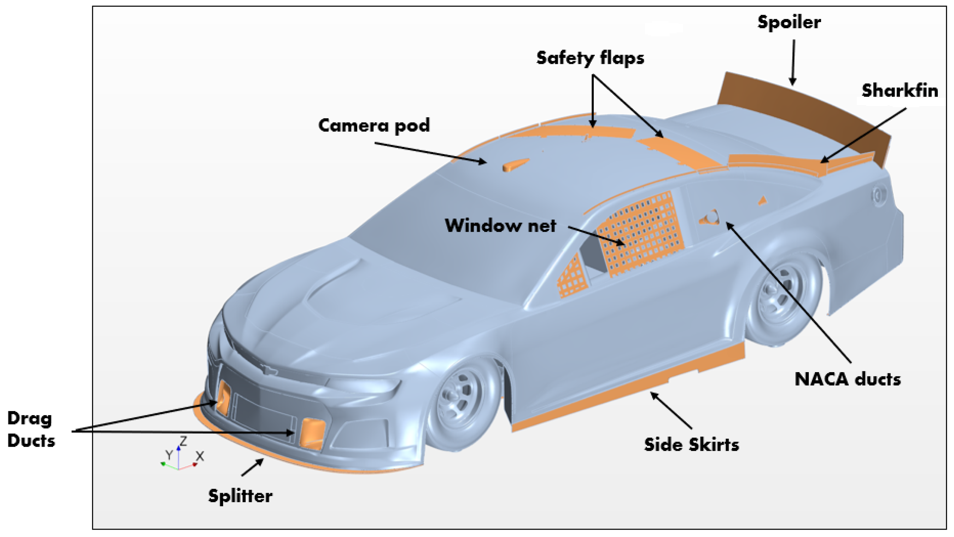
Race vehicles have many aerodynamic devices that are specifically designed for a high downforce-to-drag ratio, resulting in aerodynamic characteristics distinctly different from passenger vehicles. The Generation 6 NASCAR Cup racecar (called Gen-6 for short), which was used from 2013 to 2021, has many such aerodynamic features, as shown in Figure 1. These include a rear spoiler, roof rails, a shark fin, a very-low-ground-clearance front splitter with an underbody splitter extension panel, very-low-ground-clearance side skirts, front bypass ducts, NACA ducts for cabin and driveline cooling, a camera pod, and antennas for radio communication and GPS. Where a typical passenger vehicle normally produces a small lift with a lift-to-drag ratio of about 0.3, a racecar must achieve high-speed cornering performance, typically with down-force (or a negative lift) and having a lift-to-drag ratio of −2.0 or larger [1,2,3,4,5,6,7,30,31]. Race cars experience dynamic on-track conditions having significantly different aerodynamic behaviors between cornering and straight-line driving conditions due to the effects of high operating speeds, vertical acceleration, vehicle ride height changes, and orientation changes. A racecar on corner entry is subject to braking, while, on corner exit, it is subjected to a high longitudinal acceleration. This causes the pitch of the racecar to change in what are called dive-and-squat angles. The race vehicle experiences a significant yaw during corner entry, apex, and exit. Therefore, the vehicle’s aerodynamic characteristics must be analyzed under an envelope of yaw and pitch orientations. The existing literature covers yaw and pitch effects on generalized car shapes, such as the Ahmed body and DrivAer body, both experimentally and numerically [32,33,34,35,36,37,38]. Some limited work is also published for performance cars focusing on specific areas such as wings or using simplified geometries [39,40,41]. Very early numerical experiments using CFD as a tool focused on understanding the car performance in different conditions and were limited to very simplified, and now outdated, Gen-4 and Gen-5 NASCAR geometries [42,43,44]. Nevertheless, the work of Fu et al. focused more on the effects of turbulence parameters, boundary conditions, solver parameters, and the choice of turbulence models on the flow predictions [3,4,5,6,7].

The reader must note that a wind tunnel is an experiment by itself and is therefore susceptible to its own various sources of error. Each wind tunnel is unique and the operators have to apply corrections in order to report open-air results. The work by Fu et al. [3,4,5,6,7] and Jacuzzi [45] uses detailed Gen-6 geometries with their data validated using data collected at the AeroDyn wind tunnel. This full-scale tunnel is a closed-jet, open-return design using boundary layer suction for ground-plane simulation. A closed-jet wind tunnel, such as AeroDyn, has a high blockage ratio, requiring the application of blockage correction ratio factors [7,46]. All CFD simulations presented in this paper are validated against data from Windshear, an open-jet closed-return-type wind tunnel with a moving belt for rolling road simulation, a design that is particularly well suited for road-ready motorsport vehicles. All aerodynamic forces and moments are non-dimensionalized using reference geometric and wind velocity measurements. These non-dimensionalized forces and moments are then presented as coefficients to three decimal places. Each 1/1000th place is commonly referred to as a “count”. The Computer-Aided Design (CAD) and WT data for the Gen-6 NASCAR geometry presented in this study were obtained from a sponsor through a Non-Disclosure Agreement (NDA). Due to NDA constraints, all aerodynamic coefficients presented in this paper are non-dimensionalized using arbitrary reference values.

The challenge that CFD methodologies present to racecar simulations, highlighted by the authors in their previous studies, is that different turbulence modeling strategies within the differing CFD simulations yield significantly different flow field predictions [1,2,3,4,5,6,7]. This raises some important issues requiring further investigation. To better understand how to best apply a CFD framework to racecar simulations, one must investigate which CFD prediction methodology will result in more accurate representations of real-world conditions.

Taking this further, an investigation into which regions in the flow field demonstrate the highest discrepancy will be required. The investigation in the current paper sheds some light as to which flow features around the vehicle may be contributing the most to these discrepancies, directing future studies to those specific areas likely to produce improved simulation accuracy. To conduct these investigations, the current paper looks at the correlation between the static pressure data obtained from surface-mounted probes from the wind tunnel experiments of a racecar to the predictions obtained from different CFD simulations of the same geometry.

As mentioned earlier, WT data for a Gen-6 NASCAR racecar in three operating conditions were obtained from a sponsor. The three configurations representing the three operating conditions are listed in

Table 1. Configurations of the racecar considered in this study.

Configuration	Yaw (deg)	Splitter Gap
C1	−3.0	Low
C2	−3.0	High
C3	0.0	High

below.

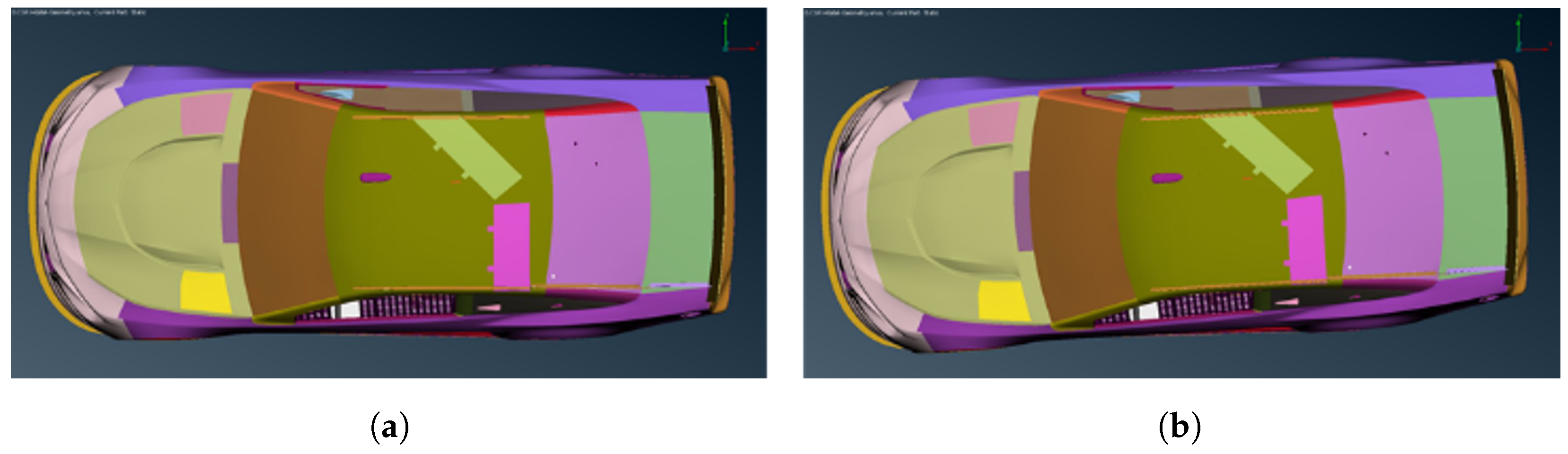
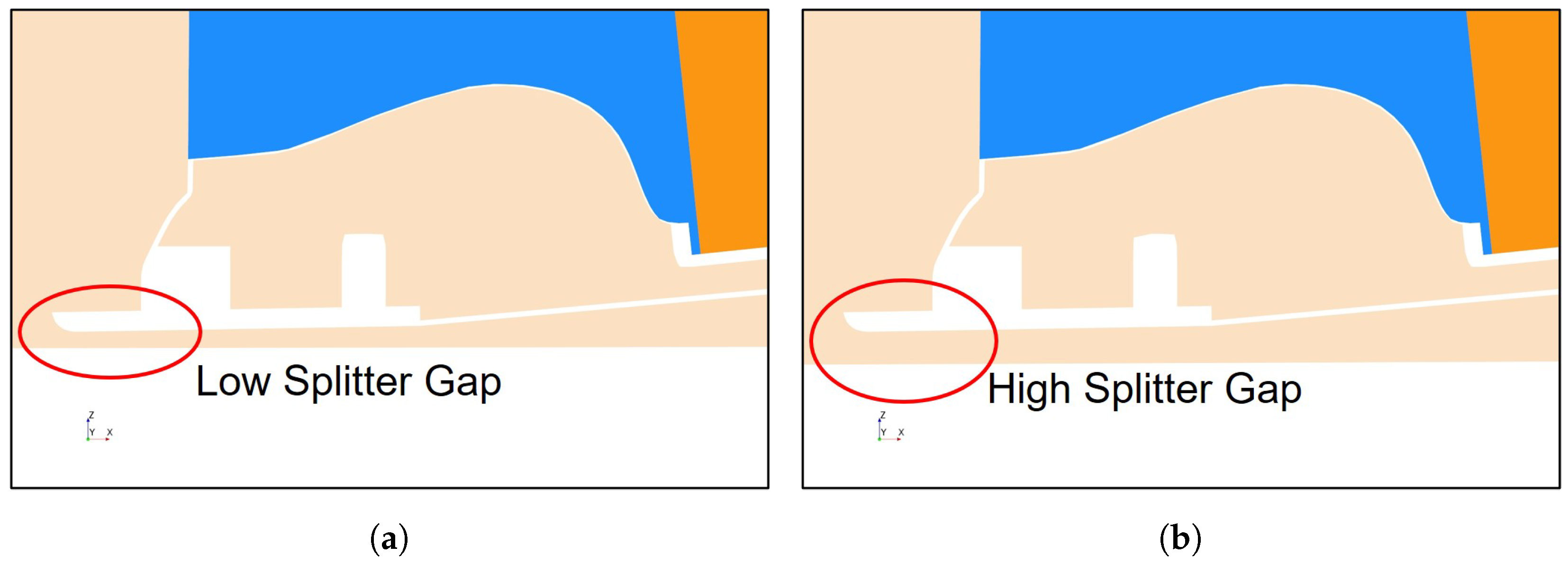
The two yaw conditions and two splitter gap conditions are shown in Figure 2 and Figure 3. Note that Figure 2a,b are top-down views of the racecar depicting the the two yaw conditions of $0deg$ and $-3deg$, respectively. Figure 3a,b are centerplane slices of the fluid domain zoomed in to show the splitter gap and show the low and high splitter gap configurations, respectively.

RANS and IDDES CFD simulations of the three configurations were run using both incompressible and compressible solvers. Simulations using the RANS and IDDES solvers will be referred to as RAS and DES, respectively, and incompressible and compressible solvers will have postfixes of “-I” and “-C”, respectively; for example, “RAS-C” will stand for a RANS simulation using a compressible solver.

Please note that this paper forms a part of the lead author Adit Misar’s doctoral dissertation work [47].

2. Methodology

The current paper contains a further analysis of the CFD experiments published earlier by the authors, with a brief description provided below. However, for further details on the computational setup for the RAS-I and RAS-C cases, the interested reader is directed to a paper by the authors’ group at UNC Charlotte [2]. This setup was then used as a baseline for developing the setup for the DES-I and DES-C cases. Again, a brief description is provided in this section, with further details on the computational setup for the IDDES cases available to the interested reader in the following paper by the authors, Misar et al. (2023) [1].

2.1. Governing Equations

The Navier–Stokes (N-S) equations are the governing equations for fluid flow. These equations represent the principles of Conservation of Mass (also referred to as the Continuity Equation) and Conservation of Momentum. For a Newtonian flow, these are given by Equations (1) and (2) respectively, using Einstein notation, where repeating index variables (i) or (j) imply summation over all possible values, e.g., ($i=1,2,3$).

$$\frac{\partial \rho }{\partial t}+\frac{\partial \left(\rho u_i\right)}{\partial x_i}=0$$

(1)

$$\frac{\partial \left(\rho u_i\right)}{\partial t}+\frac{\partial \left(\rho u_i{u}_j\right)}{\partial x_j}=-\frac{\partial p}{\partial x_i}+\frac{\partial {\tau }_{ij}}{\partial x_j}$$

(2)

where t represents time and the variables $u_i$, p, $\rho$, T, e, K, and ${\tau }_{ij}$ represent the time-dependent values of the velocity in $x_i$ direction, pressure, fluid density, temperature, internal energy, thermal conductivity, and fluid viscous stress tensor, respectively. The viscous stress tensor, ${\tau }_{ij}$, is defined as

$${\tau }_{ij}=2\mu s_{ij}$$

(3)

where $\mu$ is the fluid kinematic viscosity and $s_{ij}$ represents the instantaneous rate of the strain tensor defined as

$$s_{ij}=\frac{1}{2}\left(\frac{\partial u_i}{\partial x_j}+\frac{\partial u_j}{\partial x_i}\right)$$

(4)

The N-S equations completely and entirely describe the turbulent flow field from the largest to the smallest scales of motion. Their numerical solution requires spatial and temporal resolutions capable of resolving the so-called Kolmogorov scales. A Direct Numerical Simulation (DNS) of the N-S equations can be shown to scale with Re${}^{11/4}$ and is impractical for an engineering application at a high Reynolds number. The flow field studied in this paper has a Reynolds number of $2\times {10}^7$ and would require about 110 exabytes of memory. The computational limitations require the use of turbulence modeling.

2.1.1. Reynolds-Averaged Navier–Stokes (RANS) Approach

The Reynolds-Averaged Navier–Stokes (RANS) approach is a commonly used method for solving an engineering problem using CFD. In this approach, Reynolds decomposition is used to decompose the instantaneous velocity and pressure fields into mean and fluctuating components, mathematically expressed in the form $a_i=A_i+a_i^{\prime }$, and followed by ensemble-averaging the original N-S equations. As an example, in this convention, $u_i$, $U_i$, and $u_i^{\prime }$ represent the time-dependent instantaneous, time-averaged, and time-dependent fluctuating parts of the velocity component in the i-direction, respectively. The RANS equations are then expressed by Equations (5) and (6). Here, we describe the turbulent flow statistically in terms of the mean velocity field $U_i(\mathbf{x},t)$ and mean rate of strain $S_{ij}(\mathbf{x},t)$, instead of the instantaneous velocity field $u_i(\mathbf{x},t)$ and instantaneous rate of strain field $s_{ij}(\mathbf{x},t)$, respectively. These equations are commonly referred to as the Unsteady Reynolds-Averaged Navier–Stokes (URANS) equations.

$$\frac{\partial U_i}{\partial x_i}=0$$

(5)

$$\frac{\partial U_i}{\partial t}+\frac{\partial U_j{U}_i}{\partial x_j}=-\frac{1}{\rho }\frac{\partial P}{\partial x_i}+\frac{\partial }{\partial x_j}\left(2\mu S_{ij}-\rho \overline{u_i^{\prime }{u}_j^{\prime }}\right)$$

(6)

Let us now consider the term $-\rho \overline{u_i^{\prime }{u}_j^{\prime }}$, which is a symmetric tensor known as the Reynolds stresses. The Reynolds stress tensor introduces six additional terms into the system of equations as a consequence of the Reynolds averaging process. These six new terms now bring the number of independent variables to 10, while the system only has four equations. This is the classic closure problem found in fluid dynamics. The closure problem is often resolved using the turbulent viscosity hypothesis introduced by Boussinesq in 1877 (see Equation (7)). As per Boussinesq’s hypothesis, a relationship is needed between the turbulent stresses and the mean rate of strain, similar to the viscous stress relationship, as shown in Equation (3). However, in this case, the constant of proportionality is a fictitious flow variable, called the turbulent eddy viscosity, ${\nu }_t$, shown in Equation (7).

$$\overline{u_i^{\prime }{u}_j^{\prime }}=\frac{2}{3}k{\delta }_{ij}-{\nu }_t\left(\frac{\partial {\overline{U}}_i}{\partial x_j}+\frac{\partial {\overline{U}}_j}{\partial x_i}\right)$$

(7)

where k is the turbulence kinetic energy per unit mass, $k\equiv (1/2)\overline{u_i^{\prime }{u}_i^{\prime }}$, and ${\delta }_{ij}$ is the Kronecker delta. The determination of this flow variable ${\nu }_t$ is the central element of the turbulence modeling approach. All the various eddy-viscosity-based turbulence models found in the literature differ primarily in the way that they estimate ${\nu }_t$. All of the modern turbulence modeling approaches solve additional transport equation(s) to determine ${\nu }_t$; these types of modeling approaches are classified on the basis of the number of transport equations involved, and which transport variables are used in the modeled equations. For example, a one-equation turbulence model will involve the solution of one additional transport equation, and a two-equation $k-\omega$ modeling approach will involve transports of turbulence kinetic energy $\left(k\right)$ and a specific rate of turbulence kinetic energy dissipation $\left(\omega \right)$.

The current study uses the SST Menter $k-\omega$ (SST) [27,28] IDDES turbulence model. A short description is provided below; however, the interested reader is referred to Zhang et al. [10] and the original articles of Menter and coworkers [26,27,28] for all relevant details.

2.1.2. Shear Stress Transport (SST) $k-\omega$ Turbulence Model

The $k-\omega$ model replaces the dissipation rate $\epsilon$ used in the $k-\epsilon$ model developed by Launder and coworkers (see [48,49]) with another variable, the specific dissipation rate $\omega$, which is defined as $\omega \equiv \epsilon /k$. This model includes an additional non-conservative cross-diffusion term containing $\Delta k·\Delta \omega$ in the $\omega$ transport equation. This cross-diffusion term is used only in regions far from the wall by using a blending function. Thus, the SST model retains the advantages of the $k-\omega$ boundary layer calculation in the near-wall region while also retaining the characteristics of the $k-\epsilon$ model in the far-field freestream flow. The expressions for the eddy viscosity ${\mu }_t$ and the transport equations are given in Equations (8) to (15).

$$\frac{\partial k}{\partial t}+U_j\frac{\partial k}{\partial x_i}=\widetilde{P_k}-{\beta }^{*}k\omega +\frac{\partial }{\partial x_i}\left[\left(v+{\sigma }_k{v}_t\frac{\partial k}{\partial x_i}\right)\right]$$

(8)

$$\begin{array}{c}\frac{\partial \omega }{\partial t}+U_j\frac{\partial \omega }{\partial x_i}=\alpha \frac{1}{{\mu }_t}\widetilde{P_k}-\beta {\omega }^2+\frac{\partial }{\partial x_i}\left[\left(v+{\sigma }_k{v}_t\frac{\partial k}{\partial x_i}\right)\right]\\ +2\left(1-F_1\right){\sigma }_{{\omega }^2}\frac{1}{\omega }\frac{\partial k}{\partial x_i}\frac{\partial \omega }{\partial x_i}\end{array}$$

(9)

$$v_{\mathrm{t}}=\frac{a_{1}k}{max\left(a_1\omega ,S{F}_2\right)}$$

(10)

$$S=\sqrt{2S_{ij}{S}_{ij}}$$

(11)

$$P_k=v_{\mathrm{t}}\frac{\partial {\mathrm{U}}_i}{\partial x_j}\left(\frac{\partial {\mathrm{U}}_i}{\partial x_j}+\frac{\partial {\mathrm{U}}_j}{\partial x_i}\right)\to \widetilde{{\mathrm{P}}_k}=min\left(P_k,10{\beta }^{*}\mathrm{k}\omega \right)$$

(12)

$$F_1=tanh\left\{{\left\{min\left[max\left(\frac{\sqrt{k}}{{\beta }^{*}\omega \mathrm{y}},\frac{500v}{y^2\omega }\right),\frac{4\rho {\sigma }_{{\omega }^2}k}{C{D}_{k\omega }{y}^2}\right]\right\}}^4\right\}$$

(13)

$$F_2=tanh\left[{\left[max\left(\frac{2\sqrt{k}}{{\beta }^{*}\omega \mathrm{y}},\frac{500v}{y^2\omega }\right)\right]}^2\right]$$

(14)

$$C{D}_{k\omega }=max\left(2\rho {\sigma }_{{\omega }^2}\frac{1}{\omega }\frac{\partial k}{\partial x_i}\frac{\partial \omega }{\partial x_i},{10}^{-10}\right)$$

(15)

where $\alpha ,\beta ,{\beta }^{*},{\sigma }_k,{\sigma }_{\omega }$ and ${\sigma }_{{\omega }^2}$ are closure coefficients of the model. These are computed by the blending functions $F_1,F_2$ and the corresponding constants of the $k-\epsilon$ and $k-\omega$ models via the relationships $\alpha ={\alpha }_1{F}_1+{\alpha }_2(1-F_1)$, etc. The $a_1$ constant in Equation (10) was set to 0.31 per the STAR-CCM+ version 2020.2.1 user manual. A production limiter is used in the SST model to prevent the build-up of turbulence in stagnation regions.

2.1.3. Improved Delayed Detached Eddy Simulation (IDDES) Model

As the implementation of the LES approach is computationally expensive for automotive flows, a more practical hybrid RANS/LES approach of DES was proposed by Spalart et al. [29,50,51]. Similar in concept to the $k-\omega$ model, a switching function is also implemented by the DES approach to use LES in the regions far from the wall and RANS in the boundary layer regions. The switch between the LES solver and RANS solver is achieved via the computation of two local parameters, a local turbulent length scale, $l_T$, and a local grid size, ${\ell }_{\mathrm{LES}}$.

$${\ell }_T\equiv \frac{\sqrt{k}}{\omega }$$

(16)

$${\ell }_{\mathrm{LES}}\equiv C_{\mathrm{DES}}{\Delta }_{\mathrm{DES}}$$

(17)

A limitation of this hybrid approach is that when the numerical value of ${\ell }_T$ and ${\ell }_{\mathrm{LES}}$ reduces below a critical value, then the LES solver may be erroneously applied inside a boundary layer region. The effect of this local grid size can then be observed as a prediction of a nonphysical separation and is thus known as Grid-Induced Separation (GIS). GIS is therefore a negative consequence of the switching function and is mitigated by modifying the switching function to include a delay based on the wall-normal distance and local eddy viscosity [50]. This new approach with the modification to the switching function is called the Delayed DES or DDES. Another version of DES makes a further modification to the switching function between LES and RANS regions with the aim of providing further shielding to the boundary layer regions in high-Reynolds-number flows [51,52]. This second modification is called the Improved DDES or IDDES model, which has been used for this paper. The IDDES model includes a Sub-Grid-Scale (SGS) dependence on the wall distance that further prevents LES modeling where the wall distance is much smaller than the boundary layer thickness.

$$\tilde{\omega }=\frac{\sqrt{k}}{{\ell }_{\mathrm{Hybrid}}{f}_{{\beta }^{*}{\beta }^{*}}}$$

(18)

where $f_{{\beta }^{*}}$ is the free-shear modification factor, ${\beta }^{*}$ is an SST $k-\omega$ model constant, and the parameter ${\ell }_{\mathrm{Hybrid}}$ is defined as

$$l_{\mathrm{Hybrid}}={\tilde{f}}_d\left(1+f_e\right){\ell }_{\mathrm{RANS}}+\left(1-{\tilde{f}}_d\right)C_{\mathrm{DES}}{\Delta }_{\mathrm{IDDES}}$$

(19)

2.2. Geometry

As mentioned earlier, the geometry used in this study is a full-scale Gen-6 NASCAR racecar. The CAD file supplied by our data sponsor consists of a fully detailed geometry having high-resolution descriptions of the aerodynamic surfaces. This CAD assembly was imported into ANSA v15 and cleaned of all surface tessellation errors. Care was taken to retain all the geometric details. The fully detailed and error-free final surface consisted of 13 million triangles. This surface was then imported into Star-CCM+ and surface-meshed for CFD simulation.

2.3. Computational Domain and Boundary Conditions

A sufficiently large computational domain is required to perform an open-road CFD simulation for vehicle aerodynamics. This large domain mitigates the influence of the blockage ratio and numerical pressure waves that can occur at boundaries [2,7,53]. The test geometry was placed in a virtual wind tunnel (VWT) having dimensions of $211L\times 200W\times 200H$, with the inlet and outlet boundaries being $50L$ upstream and $160L$ downstream, where L, W, and H are the respective length, width, and height of the test geometry.

The inlet was placed on the negative x-face of the computational domain and given a velocity of 67.056 m/s (150 mph). A pressure outlet was placed at the positive x-face of the computational domain with a zero-gauge pressure specification. Fu et al. (2019) [54] studied the turbulence modeling effects on the aerodynamic characterizations of a similar Gen-6 stock racecar subject to yaw. For the crosswind simulations, Fu et al. (2019) used a zero-gradient boundary condition for the side walls. A subsequent study by the current authors (Misar, A.S. and Uddin, M., 2022) [2] shows that such a zero-gradient boundary condition poses nonphysical pressure reflections on the virtual wind tunnel boundaries. Thus, for the crosswind simulations, the upstream side of the VWT was set to a velocity inlet and the downstream side to a pressure outlet. The velocity inlets then had their velocities specified in both the x and y components to obtain the correct crosswind angle to simulate the desired yaw conditions. The inlets were given a turbulence intensity specification of 1.0%, and a turbulent length scale specification of 10 mm. In this set of simulations, the inlet velocities were given a constant magnitude. However, a synthetic velocity inlet with an oscillating magnitude, as used by Curley and Uddin [16], has been suggested to more realistically represent open-air turbulence conditions. Due to the computational expense of this approach, and a lack of relevant wind tunnel data to correlate the results, the more simplified fixed magnitude approach was applied throughout. Further discussions of the value of the Curley and Uddin approach will be discussed later.

To cost-effectively emulate a moving-ground wind tunnel test scenario, the no-slip floor was given a tangential velocity corresponding to the given freestream velocity, and the wheel rotation was modeled using a local rotation rate for each wheel. A small vertical wall was used to simulate the tire–ground contact patch while maintaining the numerical stability of the simulations [5,8,55].

A porous media strategy was developed for modeling the mass flow rates through the condenser, radiator, and fan module (CRFM) to improve the underhood flow prediction accuracy. This detail is important because the accurate prediction of the underhood airflow was found to be crucial for well-correlated force predictions [56]. The porous media modeling also includes porous baffles to simulate the front and inner grilles of the radiator ducting. Using this approach, the radiator consists of three regions: the primary cooling duct, the secondary cooling duct, and the radiator core itself. Porous media modeling was tuned using the RAS-I CFD solver and the C1 configuration in order to achieve a mass flow rate matching with high accuracy to the mass flow measurements from the wind tunnel [2].

2.4. Initialization

The flow field was initialized with the same velocity, pressure, and turbulence parameters as the inlet and outlet boundaries, i.e., the freestream velocity, a gauge pressure of zero, a turbulence intensity specification of 1.0%, and a turbulent length scale specification of 10 mm.

2.5. Discretization

The computational domain was discretized using the unstructured, hex-dominant “Trimmed Cell” meshing algorithm of Star-CCM+. This algorithm takes a reference cell size (“Base Size” within Star-CCM+) and creates cells whose size is a multiple of $2^n$ times larger/smaller than the reference cell size, where n is an integer. Volume sources were used to refine the cells in regions having high rates of change in the flow field variables. Nine volume sources were placed around the car, and a further eight were placed in regions of interest, such as the splitter and spoiler. Prism layers were used on the wetted surfaces to resolve the near-wall boundary layers. Eighteen different prism layers were used to ensure that the first node height corresponded to a wall $y^{+}<1$. The final RANS and IDDES meshes consisted of 130 and 200 million cells, respectively.

2.6. Physics Setup

The simulations presented in this paper were performed using the finite-volume solver Star-CCM+ version 2020.2.1. All simulations, unless specified otherwise, were performed using a segregated flow solver on an unstructured grid using the Semi-Implicit Method for Pressure-Linked Equations (SIMPLE) method. The $k-\omega$ SST-based IDDES turbulence model was used along with its default closure coefficients for all RANS simulations, as well as the underlying RANS model of the IDDES simulations. A two-layer all-$y^{+}$ wall treatment was used to ensure reasonably accurate boundary layer calculations in complex locations of the geometry where the $y^{+}$ was not sufficiently small.

A second-order discretization scheme was used for the diffusion terms and a second-order upwind scheme was used for the convection terms of the momentum equations. For the IDDES cases, the time step was normalized by the vehicle length $\left(L\right)$ and freestream velocity $\left(U_{\infty }\right)$. The non-dimensionalized time step of $\Delta t=0.00012\times L/U_{\infty }$ was used, which corresponds to a nominal CFL (Courant–Friedrichs–Lewy) number of around unity for near-car grids, and even smaller for the far wake regions. This $\Delta t$ has been reported as a sufficiently small time step size for automotive IDDES applications [57]; this was also verified through an earlier time step independence verification study [1]. Six inner iterations were found to be sufficient for all residuals to drop by three orders of magnitude within each time step; see [1].

2.7. Stopping Criteria and Data Averaging

The RANS simulations were run for 10,000 iterations and convergence was seen to begin after 4000 iterations. The IDDES simulations were run for 90 LETOTs, where one Large Eddy Turn Over Time (LETOT) $=L/U_{\infty }$, and convergence of force and moment coefficients was seen to begin after roughly 50 LETOTs. Based on this, all RANS results presented in this paper are from an averaging window of the last 4000 iterations (i.e., averaged between iterations 6000 and 10,000), and all IDDES results presented in this paper are from an averaging window of the last 30 LETOTs (i.e., averaged between 60 and 90 LETOTs).

2.8. Computational Resources

The authors have previously observed a significant variation in the aerodynamic coefficient predictions from the CFD of a road vehicle when simulations were carried out using a Message Passing Interface (MPI) as the parallelization tool. Thus, care was taken to maintain the same parallelization schemes and hardware consistency throughout this study [24]. All simulations were run on UNC Charlotte’s High-Performance Computing clusters using 144 processors across three nodes having 48 processors each. The RANS simulations took about 40 h to run and the IDDES simulations took about 600 h to run.

3. Results and Discussion

The three configurations, examined using the four solvers mentioned earlier (RAS-I, RAS-C, DES-I, and DES-C), give a total of 12 simulations and are presented in Table 1. Section 3.2 presents the percent difference between the force coefficients obtained from the 12 CFD cases and the corresponding WT data. Section 3.3 presents the comparison of the accumulated forces between the DES-C and RAS-C solvers. The trends presented in Section 3.2 and Section 3.3 were hinted at from the difference in $C_p$ prediction on the NASCAR surface from DES-C and RAS-C for configuration C3 in the study of Misar et al. (2023) [1]. The current paper expands the discussion to include all three configurations. Lastly, in order to ascertain which CFD prediction is closer to the WT flow field, Section 3.4 examines the $C_p$ predictions on the surface for C3 with data from DES-C, RAS-C, and WT.

3.1. Grid Independence and Data Uncertainty

To check the grid independence of the CFD predictions, all three configurations were run using three mesh sizes. The meshes were labeled as Coarse, Baseline, and Fine. The Coarse and Fine meshes were obtained by changing the base cell size by $\pm 10\%$. Thus, the Coarse mesh contained about 96 million cells, and the Fine mesh contained about 165 million cells. Figure 4 shows the variation in the drag (CD) and lift (CL) coefficients obtained by the RAS-C solver with respect to the grid size. Each subfigure shows nine data points as a percent difference with regard to the respective wind tunnel values. We can see in Figure 4a that the changes in CD predictions with the mesh are <$1\%$ for each configuration. The uncertainty in each simulation was calculated as the root-mean-square of the fluctuating component and is shown with error bars on each data point. The uncertainty in drag predictions was found to be <$0.4\%$. Figure 4b shows that the downforce is more sensitive to the grid size than the drag. The variation in CL is observed to be <$2\%$ for each configuration and uncertainty was observed to be <$0.6\%$. Thus, the baseline mesh was deemed a sufficient compromise between reasonable accuracy and the computational cost.

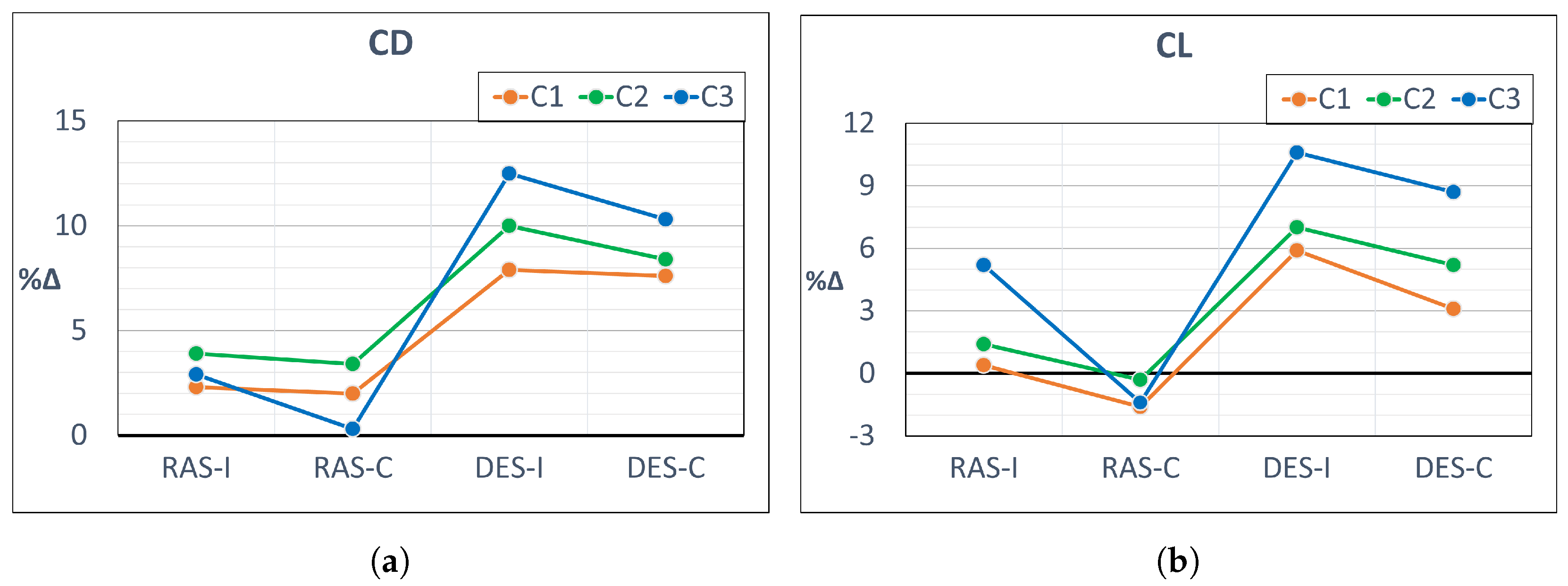
3.2. Predictions of Force Coefficients

This section will look at the aerodynamic coefficients as obtained from the 12 CFD cases in terms of their percent difference ($\%\Delta$) relative to the respective WT values. Figure 5 reveals the percent difference ($\%\Delta$) of the CFD-predicted-force-coefficients relative to the WT values in which three general trends emerge. First, both DES solvers have a greater overprediction of CD (see Figure 5a) and CL (see Figure 5b) than their RANS counterparts. This may indicate an increased pressure prediction on the front and rear-facing surfaces by the DES solvers, as well as an inability to capture the peak suction pressures on the underside of the racecar. Second, both compressible solvers have a slightly reduced percent error as compared to their respective incompressible counterparts. This may indicate a better prediction correlation by the compressible solvers in the regions most susceptible to local compressibility effects, such as the splitter suction pressure region. Third, C3 seems to have the largest variance in its predictions between the DES-C and RAS-C cases. Thus, C3 is investigated further in Section 3.4 of this paper. As a reminder of Table 1, C3 is the higher-splitter-gap, zero-yaw-angle configuration of the racecar.

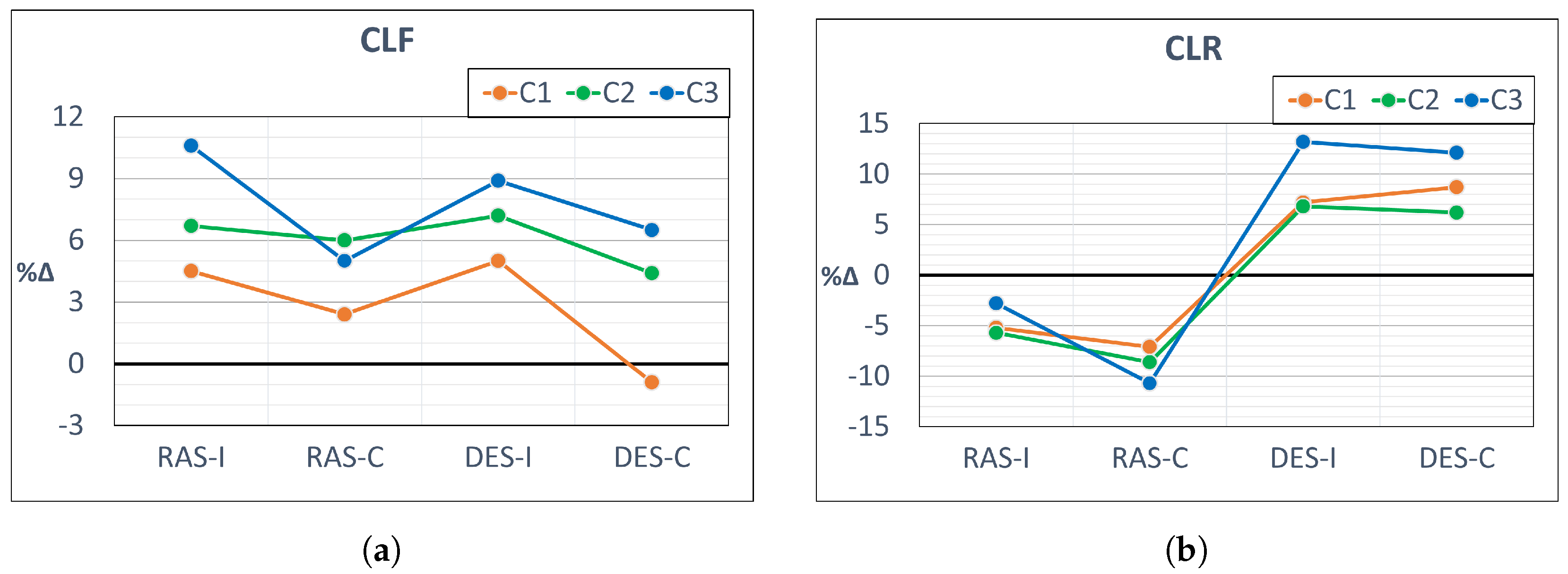
Figure 6 shows the distribution of the front and rear downforce (negative lift) of the racecar. Figure 6a shows that generally CLF is overpredicted for all cases. C1 DES-C follows the same trend as all its neighbors but has a negligible difference with regard to WT. This overprediction in CLF hints at an overprediction in the splitter suction pressure or an overprediction of $C_p$ on the hood, cowl, and windshield surfaces. In Figure 6b, it is seen that both RANS solvers underpredict CLR, while both DES solvers overpredict CLR. This could indicate an overprediction of $C_p$ on the decklid and spoiler by the RANS solvers and an underprediction of $C_p$ by the DES solvers. This change in trend in the DES solvers with regard to the RANS solvers may also be attributed to the diffusion of the underbody jet, as seen in the study of Misar et al. (2023) [1].

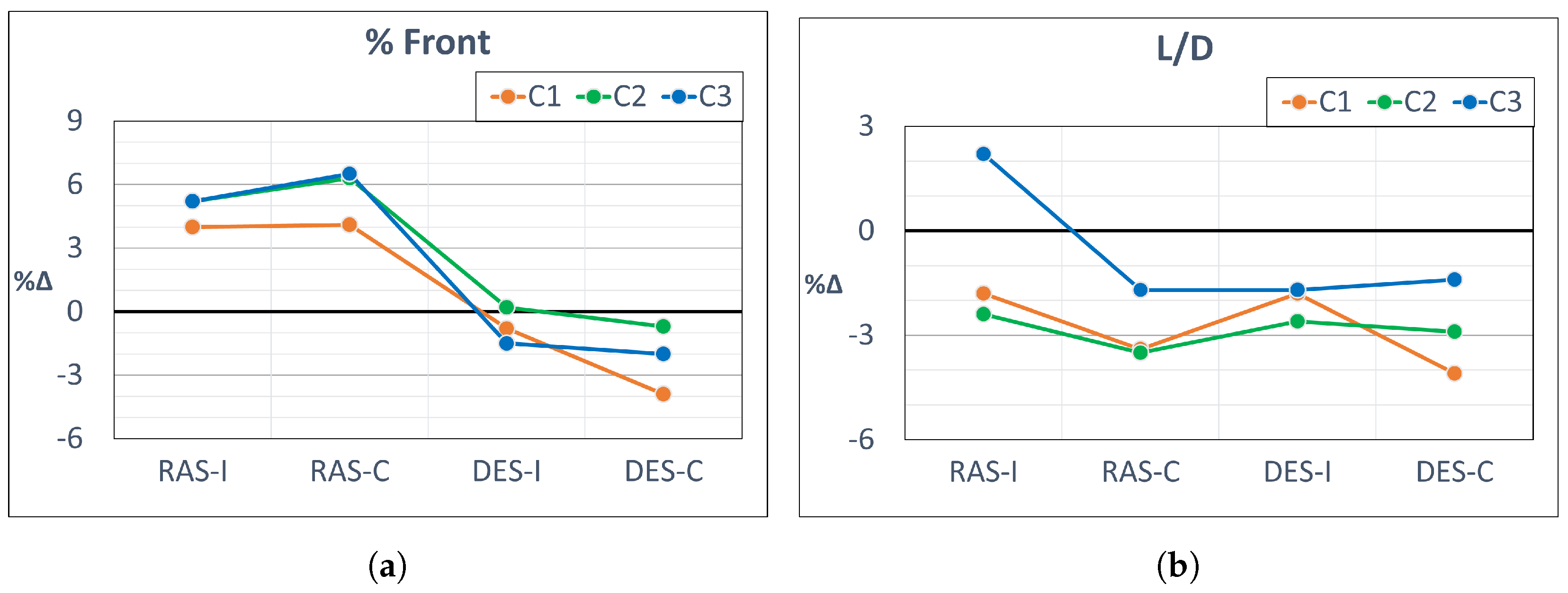
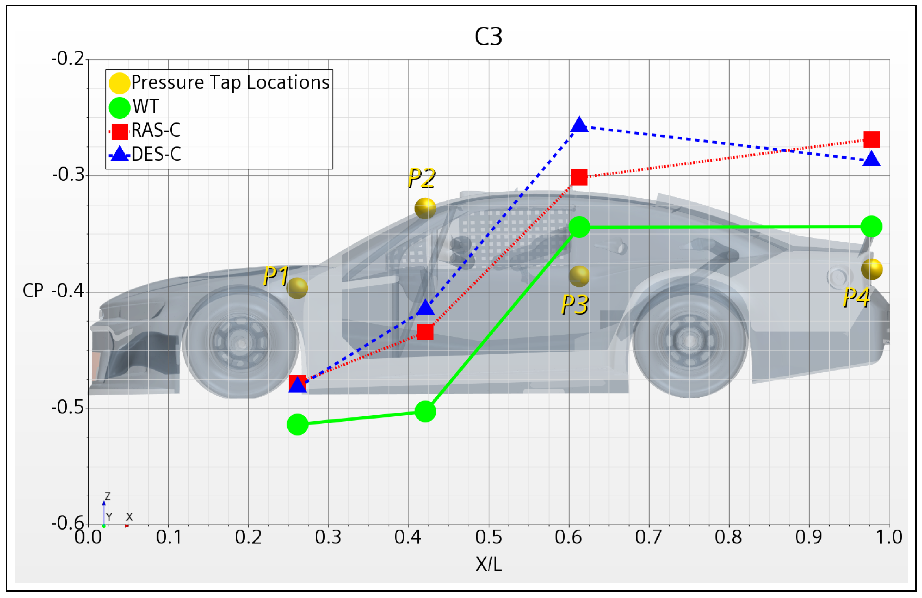
Figure 7 reports the longitudinal distribution of CL. As defined earlier, ”%_Front” defines the front-to-rear downforce balance (or a ratio of Front-lift-force to Total-lift-force ) and is shown in Figure 7a. As expected from the prior graphs of Figure 5 and Figure 6, the RANS solvers overpredict %_Front. This again points to the $C_p$ predictions on the splitter, hood, decklid, and spoiler surfaces as the possible sources of error, as these surfaces play a major role in downforce production. The DES solvers slightly underpredict the percent difference in %_Front by less than −2%, except for C1 in DES-C, which is closer to −4%. This supports the conjecture that the DES solvers are generally overpredicting $C_p$ in an equal proportion in the front and rear parts. In Figure 7b, all cases predict $L/D$ around negative 2–3% of the WT value, except the two outliers of C3 in RAS-I and C1 in DES-C; note that $L/D$ is called “Lift-to-Drag ratio”, where L and D stand for Lift-force and Drag-force, respectively. Looking specifically at Figure 7b, it can be observed that 10 of the 12 simulations report that $L/D$ results are within a narrow range between −2 and −4%. The specific physics likely producing the two outliers is not fully understood and will be discussed following additional future research pertaining to the effects of crosswind and the effects of the splitter gap height.

3.3. Accumulated Forces

Next, the accumulated aerodynamic force coefficients along the longitudinal dimension of the vehicle geometry were examined. These provided further insight into the development of the pressure field on the vehicle surface. All DES cases are plotted as solid lines and all RANS cases as dashed lines; C1, C2, and C3 configurations are shown in red, blue, and green, respectively.

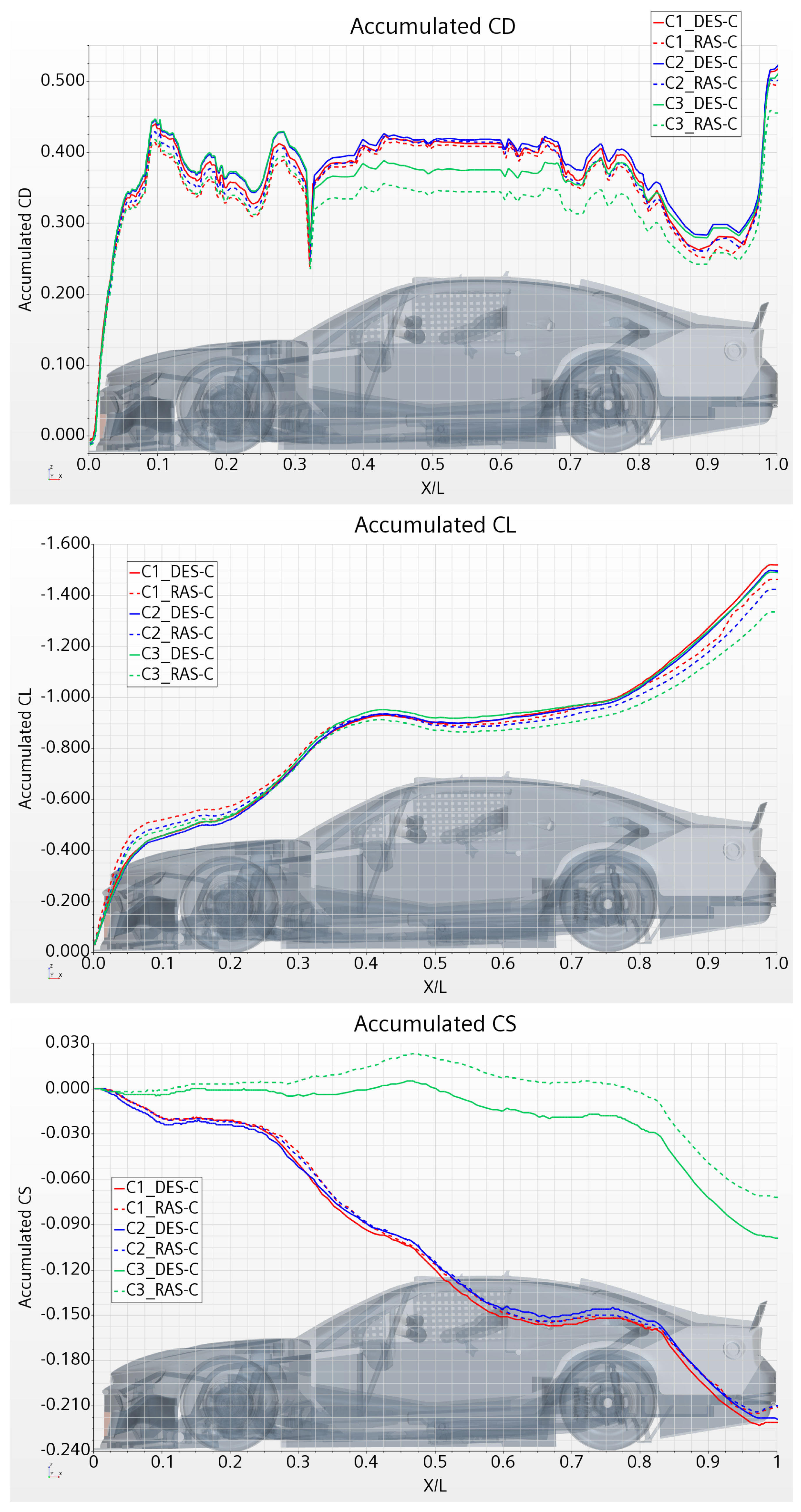
Figure 8 shows the accumulated force coefficients. In Figure 8 (Top), it is observed that all DES cases predict higher CD than the respective RANS cases. The differences occur in between location ranges from $0.05<x/L<0.30$ and $0.70<x/L<0.95$, corresponding to the hood and decklid regions, respectively. Moreover, C3 has a significant difference between DES-C and RAS-C from $0.30<x/L<0.85$. This could be a result of the diffused underbody splitter jet in the DES-C case. The diffusion of this jet may indicate higher streamwise wall shear stress in DES-C with regard to RAS-C and these may contribute to the higher friction drag. In Figure 8 (Middle), all RAS-C cases are overpredicting CL in the range $0.05<x/L<0.25$ and underpredicting CL in the range $0.5<x/L<1.0$. This is consistent with the observations in Figure 6. The front overprediction corresponds to the splitter and front diffuser geometries. The rear underprediction seems to be an effect of the underbody flow. In Figure 8 (Bottom), C1 and C2 are well matched for both the DES-C and RAS-C solvers. The largest difference is observed in the range $0.3<x/L<1.0$ from C3, which is a zero-degree-yaw configuration. The NASCAR geometry is inherently asymmetric along the longitudinal axis and this asymmetry is the cause of a non-zero sideforce even in the zero-yaw configuration. The significant prediction difference in CS between DES-C and RAS-C for C3 indicates a pressure field difference on the side surfaces. The fact that the difference starts slightly downstream of the front tires suggests an influence of the front wheel wakes.

In order to further explore the effects of solver choices, Figure 9 analyzes the differences in the accumulated force coefficients obtained using the DES-C and RAS-C solvers for all three configurations. For this, the RAS-C cases were taken as the baseline and the DES-C predictions are reported relative to the RAS-C predictions. Thus, all positive differences are overpredictions in the DES-C case and vice versa. C1, C2, and C3 configurations are shown in red, blue, and green, respectively. In Figure 9 (Top), C3 has the largest difference in CD between DES-C and RAS-C relative to the differences seen for C1 and C2. This is due to three factors: (i) a higher CD contribution from the range $0<x/L<0.075$ corresponding to the splitter and front fascia, (ii) a smaller drop near the cowl region at $X/L=0.325$, and (iii) a larger drag contribution from the spoiler located beyond $x/L=0.95$.

In Figure 9 (Middle), the highest overprediction is observed with DES-C for the C1 configuration at $x/L=0.05$. C1 is the low-splitter-gap case, and is thus expected to have a higher splitter suction compared to C2 and C3 configurations. Figure 6a shows that, for C1, DES-C had a lower CLF prediction compared to RAS-C, and Figure 9 (Middle) further indicates that the splitter suction pressures have different predictions. Moreover, the consistent downward slope of all three cases from $x/L=0.1$ to the rear indicates a strong correlation to the underbody splitter jet flow. Thus, it will be important to inspect the static pressure data from the point probes in the underbody region. C1 also seems to have an unphysical spike at $x/L=0.95$ that may be derived from numerically induced noise in post-processing the data. This is left for a subsequent investigation.

In Figure 9 (Bottom), C1 and C2 have differences of less than 10 counts. The difference arising from C3, the zero-yaw case, is very significant and highlights the need to study the probes on the sides of the vehicle. It is interesting to note that, for all three cases, the differences in CD appear downstream of $x/L=0.225$. This indicates that the wake and outwash generated from the front tires may be playing a significant role in the flow prediction over the doors and thus affecting the sideforce predictions.

To enhance the understanding of such a phenomenon, further investigation of the flow field in the near vicinity of the vehicle is required. Data on pressure and velocity were collected from this region of the flow field, allowing a more in-depth study. These data were generated from a collection of 50 CFD-generated point probes placed in the flow field. From each point probe location, five scalars, including the static and total pressure coefficients and the three components of the velocity vector, were collected. Because the corresponding WT data for these point probes are not available, the establishment of the overall veracity of the CFD simulations is required prior to the analysis of the flow field. The data will be analyzed and presented in a subsequent paper.

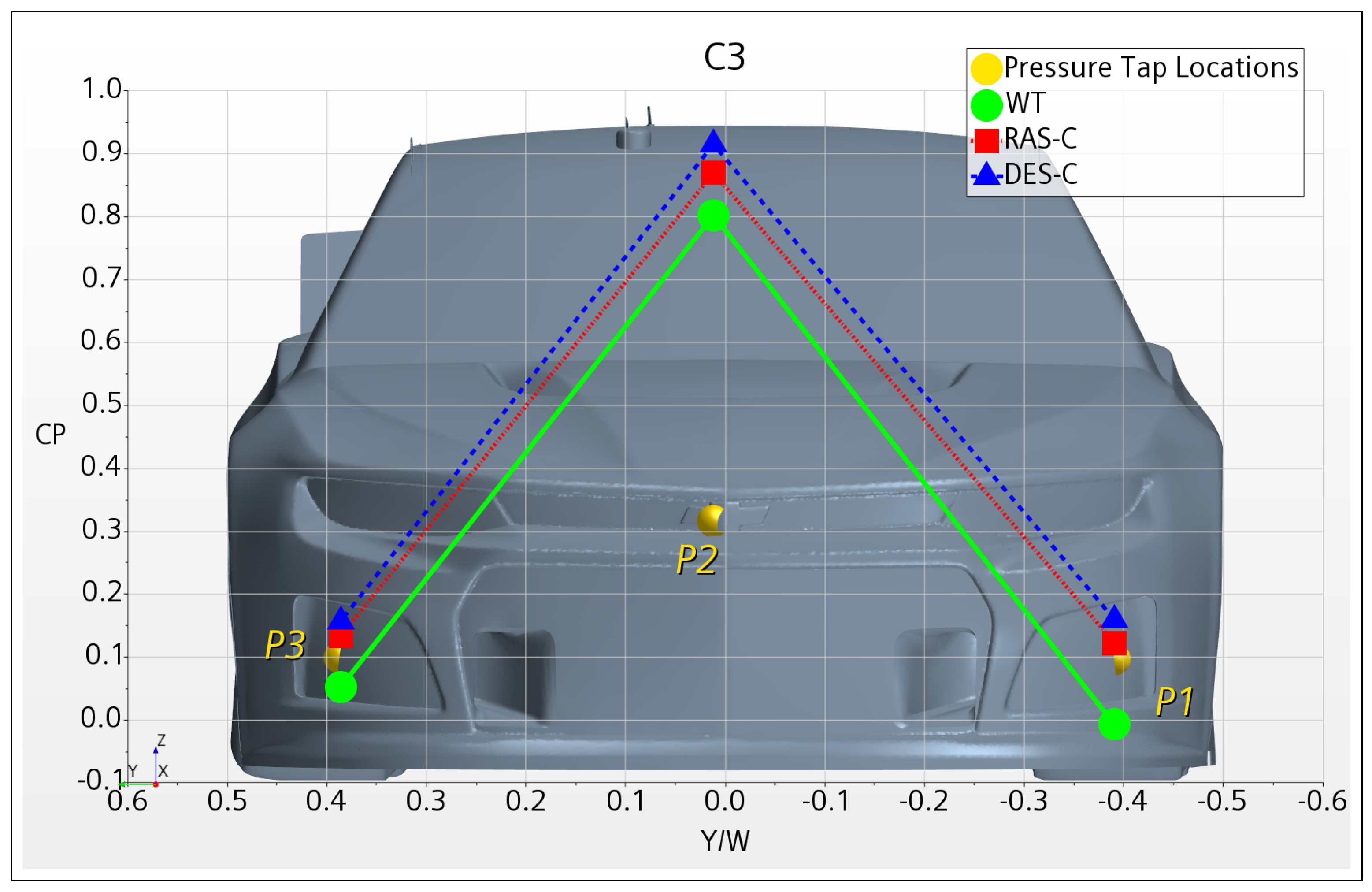
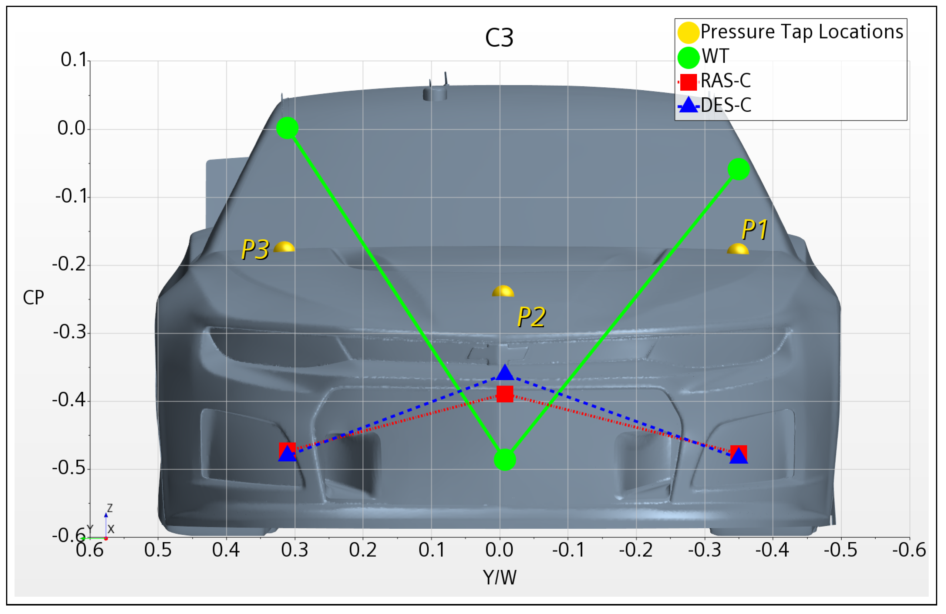
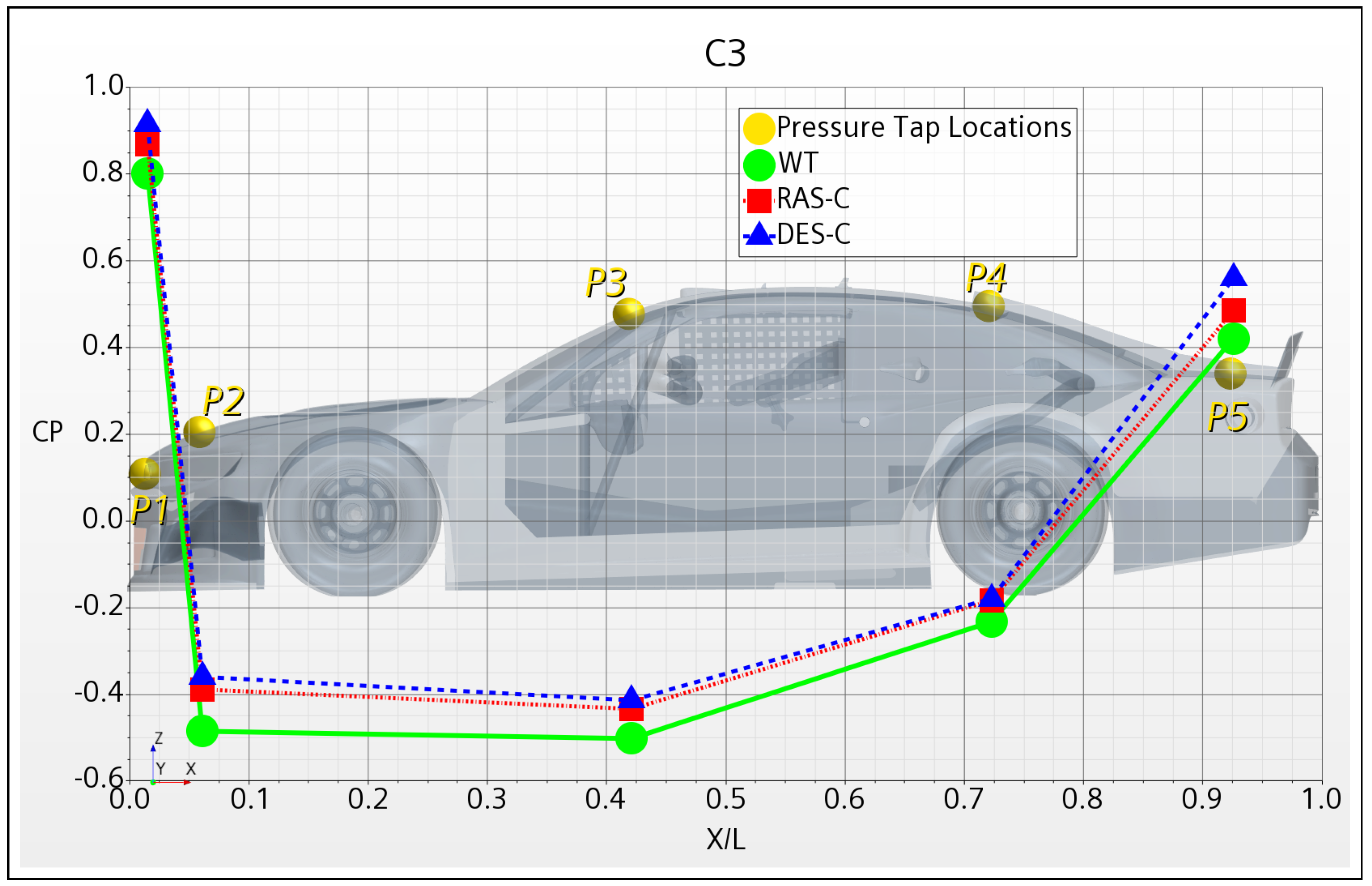
3.4. Pressure Probe Data

This section compares static pressure data on the vehicle surface for C3 as obtained from DES-C, RAS-C, and WT. Each figure has a plot overlaid on the vehicle geometry. The yellow/gold dots show the physical locations of the pressure probes on the vehicle. Each plot has its own grouping of pressure probes numbered as [P1, P2,...]. The green circles show the $C_p$ values obtained from the WT. The blue triangles show the CFD-predicted $C_p$ values from DES-C. Lastly, the red squares show the CFD-predicted $C_p$ values from RAS-C. The examination will begin by first looking at the splitter and underbody regions, then the spoiler region, the hood region, and finally the sides.

3.4.1. Splitter and Underbody Region

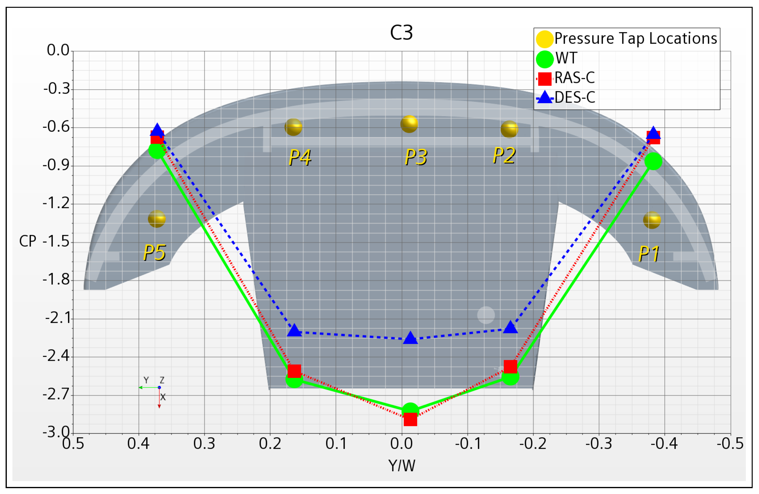
Figure 10 is a plot of the surface $C_p$ distribution on the splitter of the vehicle for C3. This region of the vehicle has the lowest ground clearance and the strongest suction pressures. Being the most upstream part of the vehicle geometry, this region has the least impact on upstream flow predictions. Towards the sides at locations P1 and P5, the predictions of WT, DES-C, and RAS-C are well correlated. RAS-C continues this good correlation at all interior locations. However, DES-C shows a significant underprediction of the suction pressure and fails to capture the peak suction pressure at the central P3 probe. This suggests that, in the DES-C flow field prediction, there may be a local separation bubble slightly downstream of the P3 probe location. Such a flow prediction was indicated in the observations of Misar et al. (2023) [1]. The impact of such a local separation bubble should be seen more clearly in the front diffuser region (also called the splitter extension panel).

Figure 11 is a plot of the surface $C_p$ distribution on the trailing edge of the splitter extension panel of the vehicle for C3. Immediately, it is seen that the WT seems to be predicting an outlier at P3, having significantly larger suction pressure as compared to the other locations (by about 25%). This seems to be an unphysical phenomenon and requires further flow field data from the WT experiment. Apart from this, a trend similar to that observed in the splitter region is seen. Towards the sides at locations P1 and P4, the values from WT, DES-C, and RAS-C are well correlated. At the interior points of P2 and P3, both DES-C and RAS-C predictions are correlated to each other, but both underpredict with regard to the WT value. This seems to suggest that, based upon the divergence from the WT values, neither CFD solver is able to accurately predict the flow acceleration. Some additional WT pitot tube information from the trailing edge of the splitter extension panel may be required to develop a complete understanding of the local flow in this region. This would allow more robust comparisons of the streamwise velocity from the different simulations.

Figure 12 is a plot of the surface $C_p$ distribution on the floor of the vehicle for C3. Generally, the floor suction pressure is underpredicted, except for the RAS-C prediction at P1. A basic understanding of Bernoulli’s Principle implies that an underprediction of underbody suction pressure indicates an underprediction of streamwise velocity in the underbody flow. This figure shows that the RAS-C prediction is better correlated to the WT data than the DES-C prediction. This is consistent with the authors’ earlier observations from a scalar of $\Delta C_P$ on the underbody surface [1]. It is also wise to remember that the WT in itself is a simulation of open-road conditions. The rolling belt used to simulate a moving ground cannot be infinitely rigid and thus may have an induced vertical oscillation due to the vehicle’s underbody suction. The pressure and velocimetric data from a coastdown test may be required to ascertain the true state of the underbody suction conditions.

Figure 13 is a plot of the surface $C_p$ distribution on the LHS floor of the vehicle for C3. At these locations, the DES-C predictions are closer to the WT values, while RAS-C is underpredicting the suction pressure at P1, P2, and P5, and overpredicting the suction pressure at P3 and P4. This is a region of the flow field where air from outside the vehicle’s footprint rolls over the edge of the side skirts and enters the underbody flow [1]. Figure 13 suggests that the transient solver of DES-C is better able to capture the impact of the dynamic flow on the local pressure field.

Figure 14 is a plot of the surface $C_p$ distribution on the RHS floor of the vehicle for C3. In the near wake of the front tires at P1 and P2, and in the region of the rear tire squirt at P5 and P6, the suction pressure is underpredicted, with the exception of P1 for DES-C. Suction pressure is overpredicted slightly upstream of the exhaust pipes at P3 and P4. Larger discrepancies exist between DES-C and RAS-C predictions at P1, P2, P5, and P6, all of which are within the influence of the tires. The tire squirt and the near-wake region contain many flow structures that have a range of frequency and length scales. Accurately predicting these regions is difficult, and the simulation setup may have a significant effect on the downstream flow structures, such as those that were captured in this examination. Different wheel rotation modeling strategies may have a significant impact on these areas [8].

Figure 15 is a plot of the surface $C_p$ distribution on the fuel cell and rear crash structures of the vehicle for C3. All CFD predictions are underpredicting the suction pressures, except for P5 in DES-C, which shows a good correlation to the WT corresponding value. At P2 and P3, RAS-C seems to be more aligned with the WT values, but both solvers have nearly identical predictions at P1 and P4.

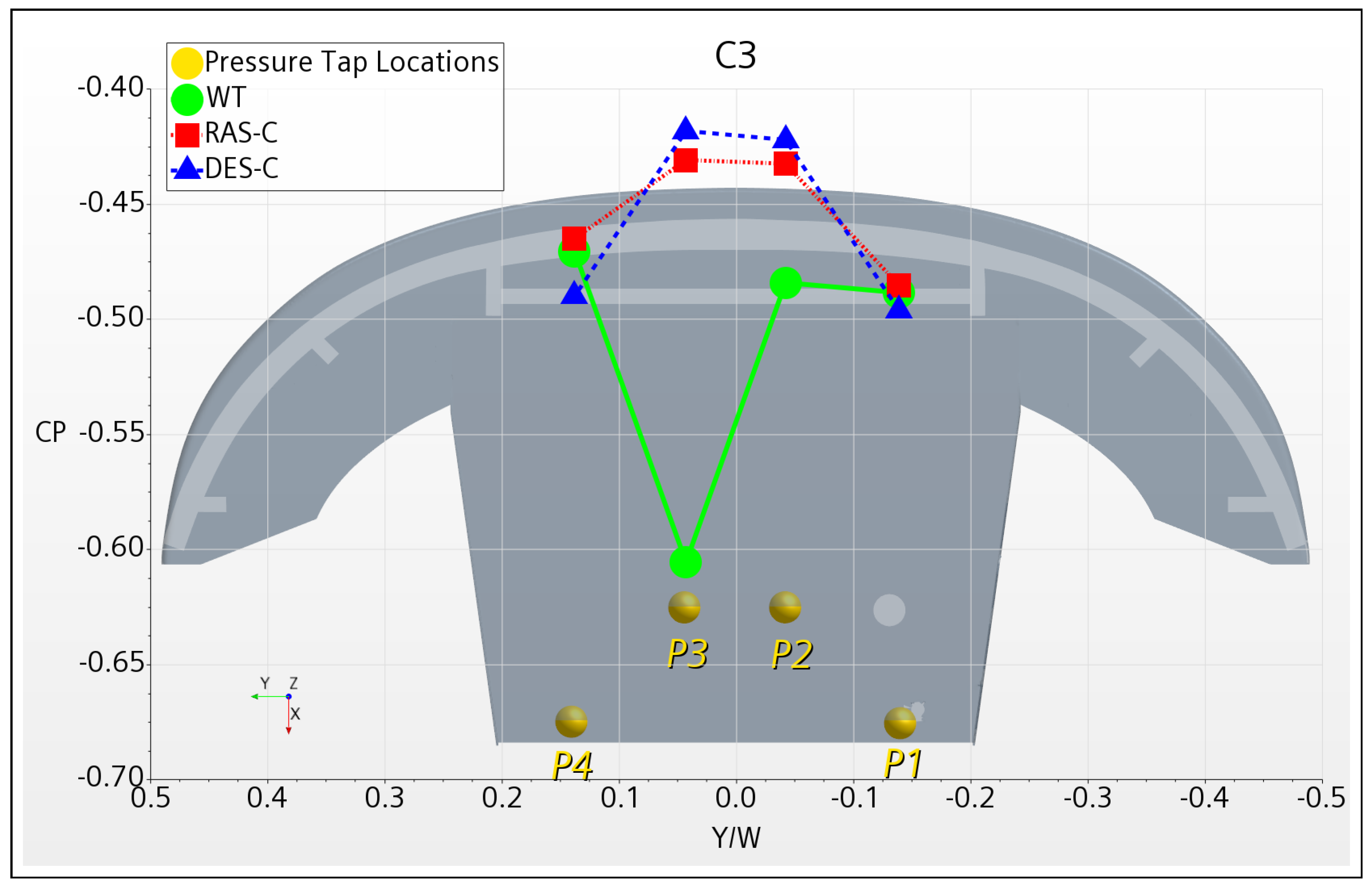
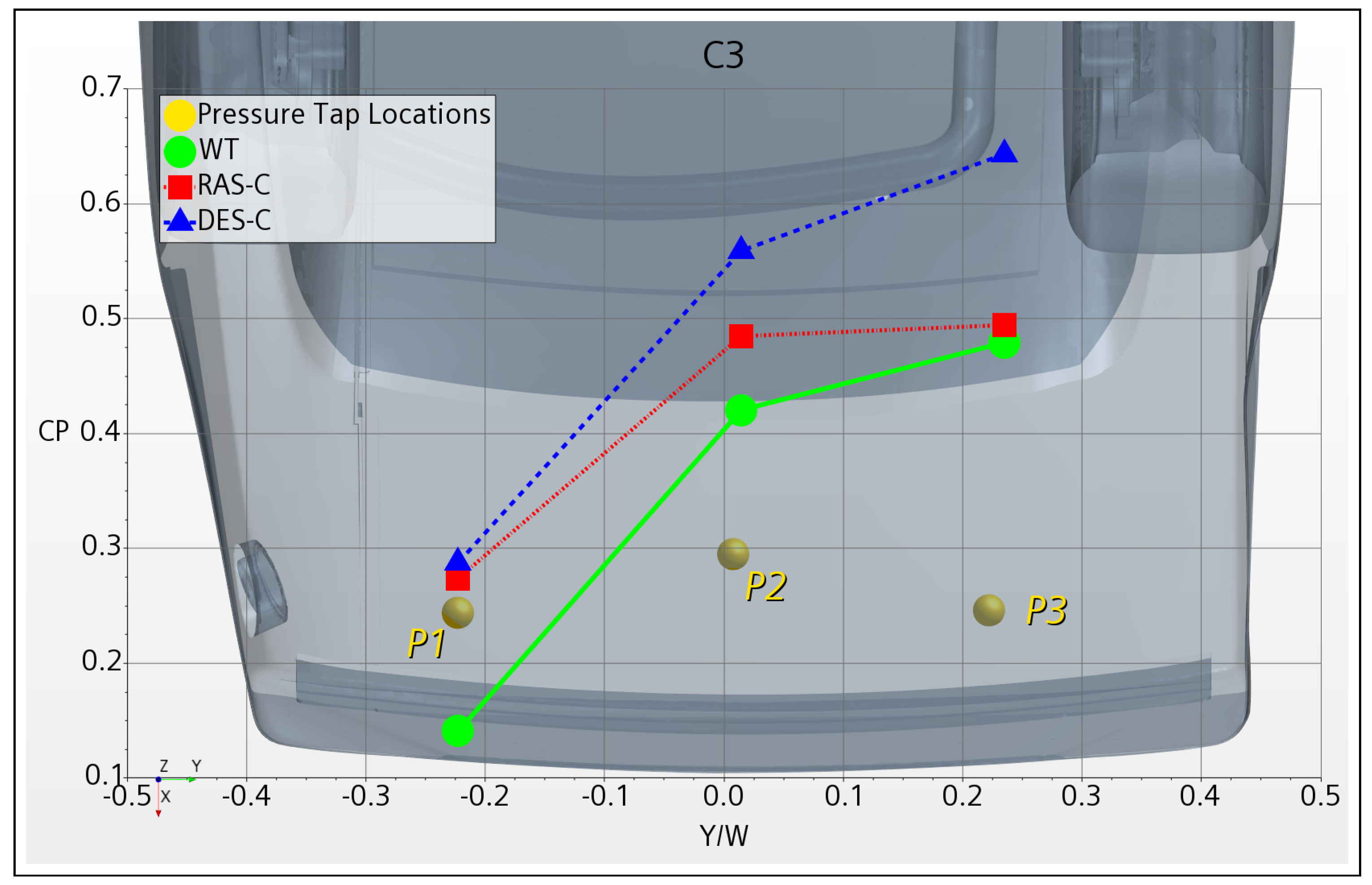
3.4.2. Spoiler Region

Figure 16 is a plot of the surface $C_p$ distribution on the rear windshield for the C3 vehicle. DES-C predicts a higher $C_p$ at all three points with respect to both WT and RAS-C. At P2 and P3, the RAS-C and DES-C predictions are very closely matched, but at, P1 RAS-C significantly underpredicts compared to both WT and DES-C. It will help the reader to know that P1 is located slightly inboard of the shark fin. Thus, the RAS-C solver seems to be predicting a much higher tangential velocity along the shark fin. These CFD predictions also help to explain why the DES-C has a higher CS prediction than RAS-C, as seen in Figure 8 (bottom) and Figure 9 (bottom).

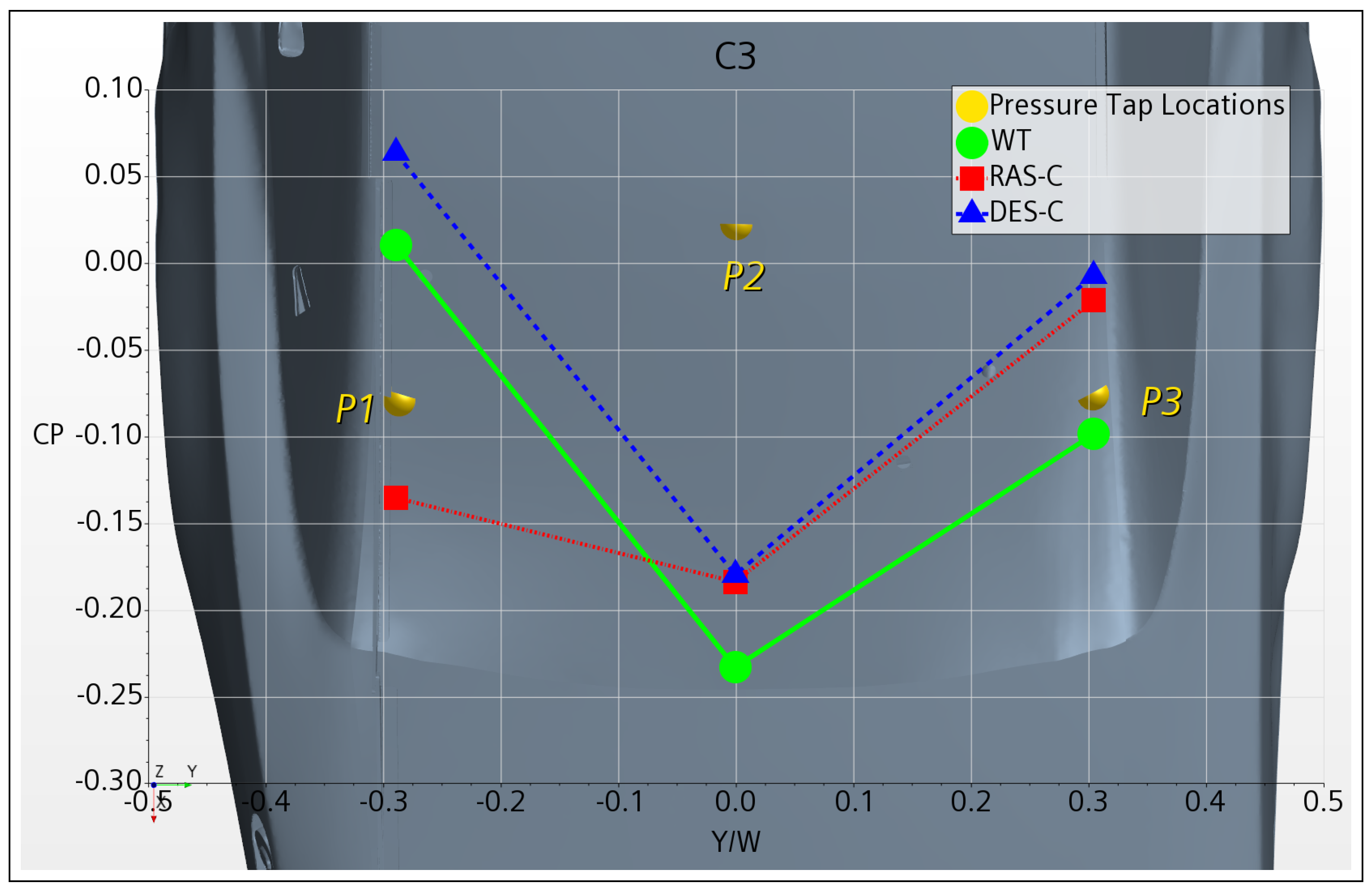
Figure 17 is a plot of the surface $C_p$ distribution on the decklid of the vehicle for C3. The P3 value from RAS-C is best correlated to WT, while all other CFD predictions are overpredicted, with DES-C having a higher overprediction than RAS-C. It was observed by Misar et al. (2023) [1] that RAS-C predicted a smoother flow in this region, whereas the DES-C flow field predictions indicated many more localized separation bubbles. In this study, RAS-C is better correlated with the limited WT surface pressure data available.

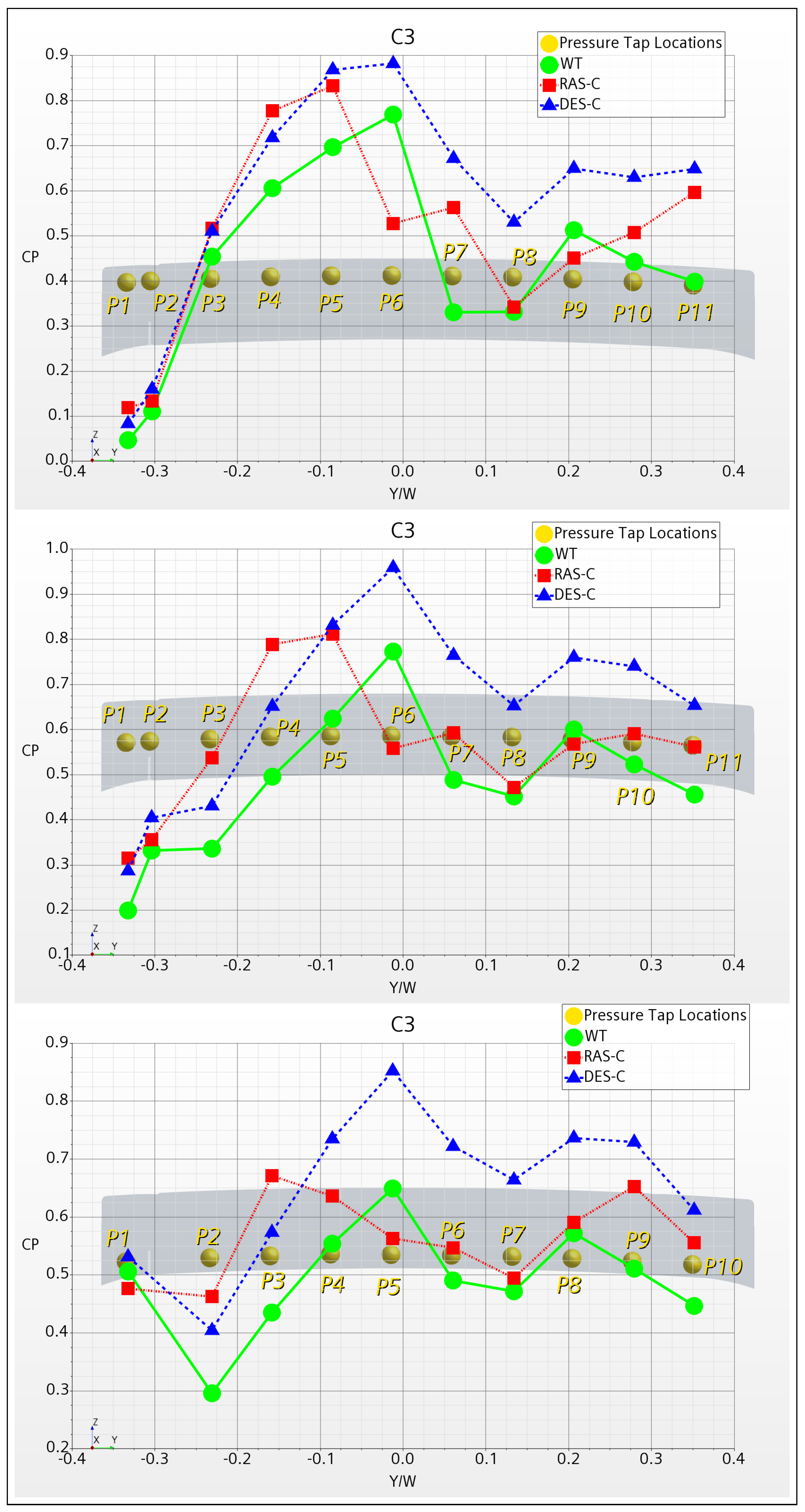
Figure 18 is a plot of the surface $C_p$ distribution on the spoiler of the vehicle for C3. The 32 physical pressure probes used in the WT are organized into three rows: (a) top, (b) middle, and (c) bottom. The viewpoint is from the rear looking forward, i.e., the RHS of the racecar is on the RHS of the plot.

On the top row, P1, P2, and P3 for both DES-C and RAS-C are well correlated to the WT values, and RAS-C has an additional well-correlated prediction at P8. DES-C has a significant overprediction with regard to WT from P4 to P11. The RAS-C predictions share this trend, except for locations P6 and P9, which are underpredicted. Both DES-C and RAS-C have similar predictions for the shark fin side from P1 to P5. From P6 to P11, DES-C significantly overpredicts relative to RAS-C. These locations are directly downstream of the decklid discrepancies seen in Figure 17. Thus, it may be that the flow features emerging from the C-pillar region are being resolved differently in the DES-C and RAS-C methods. As mentioned earlier, the flow field investigation is left for a subsequent paper.

On the middle and bottom rows, again, these general trends continue, particularly the tendency of DES-C to overpredict $C_p$ at locations P5-11 with regard to both RAS-C and WT values. This helps to explain the higher CD and CLR predictions of DES-C seen in Figure 5a and Figure 6b, respectively. However, RAS-C is also generally overpredicting $C_p$ with regard to the WT values in Figure 16, Figure 17 and Figure 18. RAS-C also underpredicts $C_p$ with regard to the WT values in Figure 15. These predictions by RAS-C would suggest an overprediction of CLR similar to DES-C, but, in fact, it can be seen from Figure 6b that RAS-C underpredicts CLR. From Figure 8 (middle) and Figure 9 (middle), the underprediction of CLR by RAS-C is mostly from the range of $0.7<x/L<1.0$. This suggests an influence of the rear wheel wake on the underbody flow affecting CLR. Again, the flow field investigation is left for a subsequent paper.

3.4.3. Hood Region

Figure 19 is a plot of the surface $C_p$ distribution on the front fascia of the vehicle for C3. Both CFD solvers are overpredicting the surface $C_p$ at all three points with respect to the WT values, with a greater overprediction seen in DES-C relative to RAS-C. These overpredictions contribute towards the higher CD predictions seen in Figure 5a. This suggests that CFD is overpredicting the stagnation region and overpredicting the mass flow rate through the front bypass ducts, the front grille, and the splitter region. As a reminder, the front grille porosity was tuned using the anemometer data from WT, utilizing the RAS-I solver for all three configurations. For C3, the radiator mass flow rate changes by less than 2% across all four CFD solvers. Further understanding and refinement of this region would be possible with enhanced experimental data, collected from additional WT pitot tubes and anemometers located in the front drag ducts. Moreover, the DNS work of Curley and Uddin (2015) using a surface-mounted cube suggests that the use of a steady inlet velocity can result in wake prediction inaccuracies [16]. All the simulations presented in this paper use such a steady inlet velocity and overpredict the drag. The authors thus recommend further investigation of the Curley approach, using a perturbed inlet velocity for better turbulence simulation, to improve the drag prediction of IDDES simulations.

Figure 20 is a plot of the surface $C_p$ distribution on the hood of the vehicle for C3. At the central P2 location closer to the nose of the vehicle, both CFD solvers are slightly underpredicted in suction pressure. This suggests a slower streamwise velocity as the flow comes over the leading edge of the hood. This may be a consequence of the mass flow redistribution suggested by the front fascia data seen in Figure 19. The outward locations P1 and P3, located on the hood flaps near the cowl region, have a significant overprediction of the suction pressure. WT has a $C_p$ value close to zero at these locations; this implies a velocity magnitude close to the freestream value as the static pressure is very close to the ambient air pressure. However, both CFD solvers predict significant suction pressure at these points. This suggests that the cowl stagnation bubble may be underpredicted in CFD.

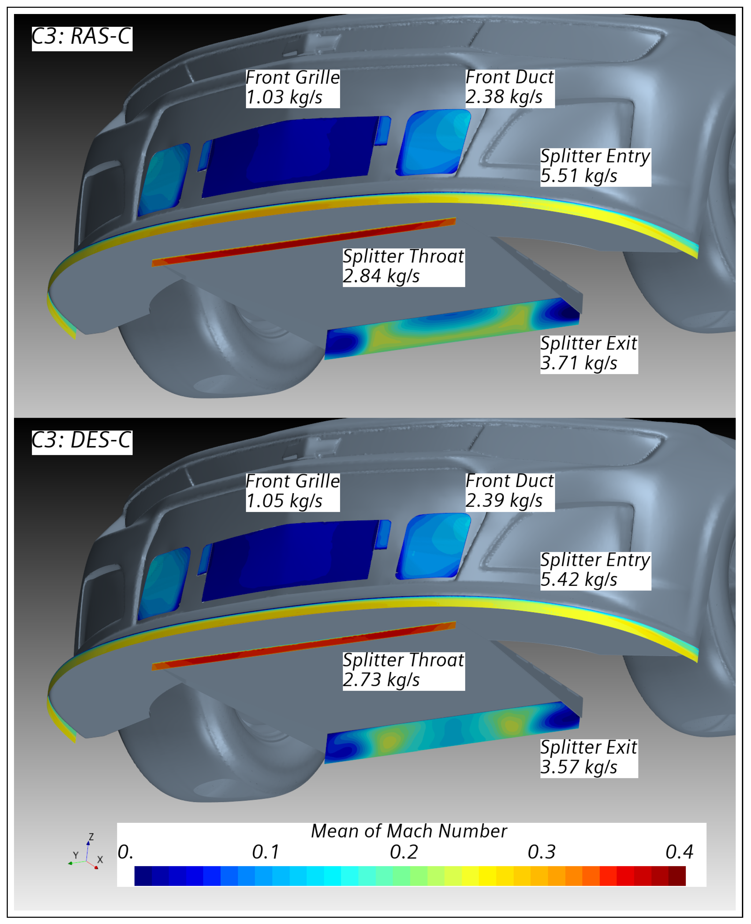
Proper resolution of the mass flow rates through the CRFM module is crucial for accurate and reliable force coefficient predictions [1,56]. To develop a deeper understanding of the mass flow trends suspected from the analysis of Figure 19 and Figure 20, we observe the mass flow rates through the front grille, the front drag ducts, and underneath the splitter. Figure 21 is a scalar showing the Mach number distribution and mass flow rates through these planes. Figure 21 indicates that DES-C has a higher mass flow rate through the front grille and front drag ducts by 0.03 kg/s, or 0.9% more than the RAS-C prediction. WT anemometer data show that the radiator mass flow is exactly in between the RAS-C and DES-C predictions. This small difference, if considered in isolation, has the effect of reduced cooling drag prediction in the DES-C case. Similarly, DES-C has a lesser mass flow rate through the splitter entry region by 0.09 kg/s, 1.6% less than the RAS-C prediction. Again, at the splitter throat and exit, DES-C has a lesser mass flow rate prediction by 3.9% and 3.8%, respectively. Taken in isolation, this would imply a reduced CLF in DES-C. However, DES-C relative to RAS-C has more mass flow through the radiator and front bypass ducts and reduced mass flow through the splitter region. Thus, DES-C is forcing more air around the front fascia, causing the higher $C_p$ prediction on the front fascia and hood regions. This is consistent with observations in Figure 19 and Figure 20, as well as in the surface $C_p$ observed in the authors’ earlier study [1].

Figure 22 is a comparison of the surface $C_p$ distribution on P1 (engine filter), P2 (roof front), P3 (cabin filter), and P4 (rear fascia) as obtained using RAS-C and DES-C solvers against WT measurements. Consistent with the observations so far, both CFD solvers are underpredicting the suction pressures at all points. The underpredictions at locations P2 and P4 contribute towards a reduced CD prediction. This underprediction of the suction pressure at location P4 is an observation consistent with those of Zhang et al. [10]. The most significant discrepancy was seen at P3, suggesting that the pipe flow through the cooling ducts may need further validation with anemometer data. It also suggests that DES-C is predicting higher frictional losses through the cooling ducts.

Figure 23 is a plot of the surface $C_p$ distribution on the upperbody centerline of the vehicle for C3. P1, P2, P4, and P5 can be seen in Figure 16, Figure 17, Figure 19, and Figure 20, respectively. P3, on the front windshield, shows the same trend as the other four points. This suggests that the entire upperbody flow prediction in CFD may have excessive skin friction or wall shear stress. Thus, the wall modeling in terms of both wall roughness and boundary layer growth needs to be studied in greater depth. Moreover, as the locations shown here have a higher $C_p$ prediction relative to WT, they contribute to the higher CL prediction seen in Figure 5b, with the predicted CL being higher for DES-C relative to RAS-C.

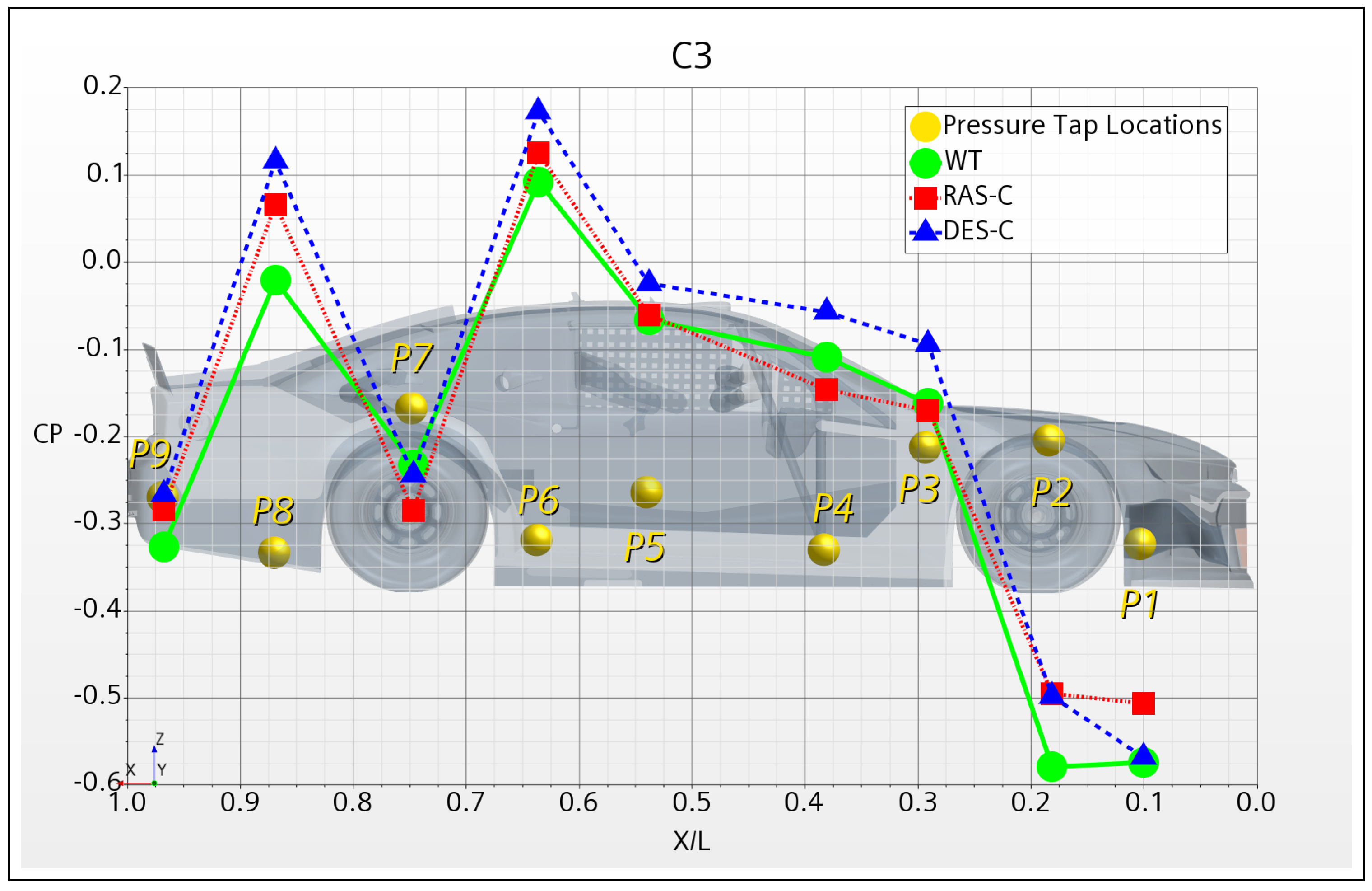
3.4.4. LHS and RHS Regions

Figure 24 is a plot of the surface $C_p$ distribution on the LHS of the vehicle for C3. DES-C is overpredicted at P1 and P6 but underpredicted at P3-5 and P7-9. RAS-C is overpredicted at P1, P4, and P6 but underpredicted at P9. The P1 overprediction of the suction pressure in both CFD solvers again suggests more mass flow coming across the front fascia. Verification of this hypothesis requires anemometer or pitot tube data at appropriate locations. DES-C and RAS-C are in good correlation with each other at P2 and P5-9. At points P3 and P4, the influence of flows over the hood region, and the turbulent wake coming from the front left tire, has to be considered. This requires a further study of the effects of wheel rotation modeling and flow field validation data. In general, it was seen that the DES-C predictions were further away from the WT values than the RAS-C predictions. This indicates a greater CS discrepancy in the DES-C solver.

Figure 25 is a plot of the surface $C_p$ distribution on the RHS of the vehicle for C3. DES-C is overpredicted at P6 and P8 but underpredicted at P2-5 and P9. RAS-C is overpredicted at P4, P5, P7, and P8 but underpredicted at P1 and P9. The trends and effects seen here are similar to those seen in Figure 24. In general, DES-C has more positive $C_p$ predictions than RAS-C for points P3-P9 in Figure 24 and Figure 25. These are contributing to the higher CS prediction of DES-C seen in Figure 8 Bottom.

4. Conclusions

In this paper, the pressure field predictions on the surface of a detailed, full-scale, Gen-6 NASCAR racecar in three configurations using RANS and IDDES turbulence modeling approaches in both incompressible and compressible modes were investigated. The force and moment coefficients were validated against wind tunnel data from WindShear. This facility utilizes an open-jet, closed-return configuration with a rotating belt for moving-ground simulation and boundary layer suction to minimize any boundary layer buildup upstream of the rolling belt. It was found that all RANS cases had drag and lift predictions within 0-5% of wind tunnel predictions, whereas the IDDES cases predicted the drag and lift to be within 3-13% of the wind tunnel predictions. Additionally, it was found that, in both turbulence modeling approaches, the compressible solver reduced the prediction discrepancies by up to 3% for both drag and lift predictions relative to the incompressible solver predictions. Hence, in this paper, the $C_p$ predictions between the DES-C and RAS-C turbulence modeling approaches were investigated. A detailed comparison of the predictions between compressible and incompressible solvers is left for a future study by the authors.

As it was found that configuration C3 had the highest discrepancy between the RANS and IDDES turbulence modeling approaches in the compressible mode, this configuration was chosen for further investigation. This was done by studying the $C_p$ distribution on the surface of the racecar via data experimentally collected from 95 static pressure probes located on a full-scale wind tunnel model. It was found that DES-C was unable to capture the peak suction pressure underneath the splitter. DES-C also predicted higher $C_p$ relative to RAS-C on the front fascia, hood, decklid, RHS of the spoiler, and fuel cell surfaces. These differences contributed to the DES-C solver overpredicting both CD and CL. The uniform DES-C overpredictions of $C_p$ around the racecar resulted in %_Front predictions very well correlated to the wind tunnel values. In contrast, RAS-C produced net CL predictions well correlated to the wind tunnel values. However, this correlation was a result of cancellation errors in CLF and CLR predictions, with the Front/Rear balance being significantly in error by 4–6%. Further, both DES-C and RAS-C struggled to predict the correct suction pressure values in the underbody flow. While this helps to explain the overprediction of CLF and CLR by the DES-C solver, the underprediction of CLR by RAS-C is not fully explained by this investigation. For RAS-C, the source of underprediction in CLR may be influenced by the rear tire wakes and the inward flow across the side skirts. Both solvers also had significant discrepancies in predicting the $C_p$ on the decklid and spoiler surfaces; this points to the flow over the rear windshield and C-pillars being resolved differently. These predictions require a further investigation of the associated flow structures.

Finally, it was found that in some regions, both DES-C and RAS-C had $C_p$ predictions well correlated relative to each other, but with both having discrepancies relative to the wind tunnel predictions. These regions were the outer edges of the splitter, the trailing edge of the splitter extension plate, the RHS side skirts around the exhaust manifold, the fuel cell, the rear windshield, the shark fin side of the spoiler, the front fascia, and the rear fascia. This suggests that the $C_p$ predictions could benefit from further tuning of the CFD framework, such as the closure coefficients of the $k-\omega$ turbulence model.