Analogy between Turbulent-to-Vortex Shedding Flow Transition in Fluids and Ductile-to-Brittle Failure Transition in Solids

Abstract

By using complex potentials, some light is shed on the analogy between the singularity problems arising in fluid and fracture mechanics—in particular, those concerning plane irrotational flows around sharp obstacles and plane elasticity in cracked bodies. Applications to two equivalent geometries are shown: a thin plate transversally immersed in a uniform flow and a crack subjected to uniform out-of-plane shearing stress at infinity (Mode III). The matching between the fluid velocity field and the shearing stress field is consistent with the hydrodynamic analogy. Aside from the Reynolds criterion for the natural laminar-to-turbulent transition, a velocity-intensity factor criterion is defined to predict the forced turbulent-to-vortex-shedding fluid-flow transition (forced transitional flow) generated by a transversal plate obstacle. It is interesting to remark that the velocity-intensity factor presents physical dimensions intermediate between those of a velocity and a kinematic viscosity. In addition, it will be demonstrated that size affects the occurrence of natural-to-forced transitional phenomena in fluids, in a strict analogy to the scale-dependent ductile-to-brittle failure transitions in solids.

1. Introduction

The analogy between plane elasticity and incompressible plane flow problems is well-known—both phenomena being governed by analogous field equations [1,2]. From a different point of view, dimensional analysis [3] allows one to define dimensionless numbers both in hydraulics and in fracture mechanics: as the Reynolds number, $Re$, predicts the laminar-to-turbulent transition in different fluid-flow situations [4], so the brittleness number, $s$, governs the ductile-to-brittle transition in solids [5].

Concerning the analogy between plane problems, viscous flows can be regarded as the fluid dynamics equivalent of nonlinear phenomena in solid mechanics. In the case of extreme ductility, i.e., when $E^{*}/E\to 0$ ($E^{*}$ being the Young’s modulus of the hardening material and E the Young’s modulus of the elastic material), the stress-function representing the yielded region becomes biharmonic [6,7]. Such perfectly plastic behavior appears to be similar to that of plane creeping flows―dominated by viscous forces―where a biharmonic equation for the stream function comes from assuming very small Reynolds numbers, $Re\to 0$, in the Navier–Stokes equation [8,9].

On the other hand, anti-plane shear problems in linear elasticity are governed by the Laplace equation [10]. Something analogous happens at the other extreme of plane flow, i.e., for irrotational and inviscid flows, where a velocity potential fulfilling the Laplace equation can be defined [11]. The outlined analogy has been further emphasized by the hydrodynamic analogy between potential flow and elastic torsion problems, where the shearing stress field of a linear elastic beam is represented by the velocity field of an ideal fluid, i.e., inviscid and incompressible, over its cross-section [12].

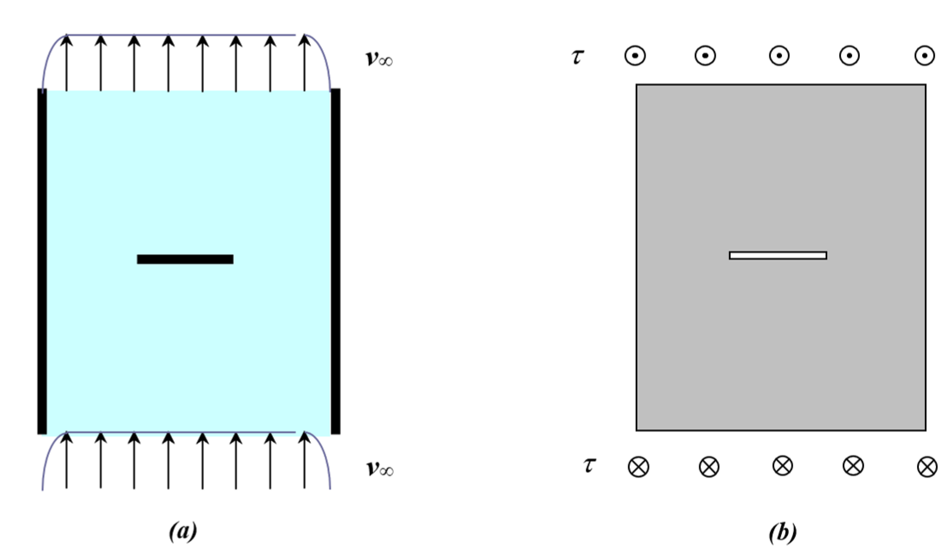
In this context, the hydrodynamic analogy can represent a heuristic device for visualizing the stress intensification around the tips of cracks or sharp re-entrant corners. In other terms, a thin or sharp-edged obstacle transversally immersed in a plane potential flow corresponds to a Griffith crack subjected to an anti-plane mode of deformation.

There are crack problems where yielding and inelastic effects are confined to a small-scale region (compared to crack and body sizes) around the crack tip [6,7,10,13]. Under these conditions, linear elastic fracture mechanics is adequate to address the problem of stress redistribution in the cracked body. Similarly, in low-viscosity flows after an obstacle, viscous effects such as vorticity―a prerequisite for turbulence―are confined to a thin boundary layer around the surface of the object, and to a wake behind it. Outside such boundary layers and wakes, the flow is treated as inviscid and irrotational, being accurately described by potential flow theory [1,14,15].

When a certain critical condition is reached, stressed bodies collapse, whereas laminar flows transit to turbulence. In both cases, there is a phase change or medium separation, in the form of newly created fracture surfaces in solids and breakdown of streamlines, leading to an eventual transition to turbulence in fluid flows.

When a structure is initially uncracked or crack-insensitive, failure by plastic-flow collapse intervenes when the applied stress reaches the material yield strength. Fracture, or separation collapse, occurs instead in a cracked structure, where lower applied stresses are sufficient to extend the crack due to the stress intensification near the crack tip [3,10,13].

As regards pipe flows, the laminar-to-turbulent transition occurs ‘naturally’, i.e., without any forcing obstacle, when a critical Reynolds number, $R{e}_C$, is reached (experimental observations show that $R{e}_C=2300$ [4]). However, the laminar-to-turbulent transition can be also forced at low Reynolds numbers, i.e., for $Re<R{e}_C$, by obstacles introduced into the flow [16,17]. Namely, low inlet velocities are sufficient to trigger a local transition to turbulence behind an obstacle for nominally laminar flows.

Although flow instabilities may occur in the wake behind obstacles of any shape, the presence of sharp edges gives rise to sudden fluid accelerations and decelerations, where the inertia of the moving fluid will favor a consequent fluid separation and vortex shedding from the bluff body. Analogously to the lines of force near the crack tip, streamlines converge and diverge rapidly around sharp-edged obstructions, resulting in a locally intensified fluid velocity. Hence, a velocity-intensity factor, $K$, may be properly introduced using a fracture mechanics approach. It is expected that, above a certain limit value $K_C$, the inertial forces due to sudden changes in the flow direction cause the breakdown of streamlines, and consequently, vortex shedding. Such a critical value, $K_C$, may be regarded as analogous to the fracture toughness.

The purpose of the present paper is to emphasize the analogy between the two problems of linear elastic fracture mechanics and of potential flow illustrated in Figure 1, namely, the uniform flow past a transversal thin plate and the plane cracking under uniform out-of-plane loading. By this strong analogy, a new dimensionless number emerges in the following, which can govern the turbulent-to-vortex-shedding fluid-flow transition.

2. Potential Flow around a Transversal Thin Plate

Let us consider the sourceless and irrotational plane flow of an ideal fluid of density $\rho$, whose velocity vector is $v=v_x e_x+v_y e_y$. Recall that, for a sourceless incompressible plane fluid flow of velocity $v$, the continuity equation $\dot{\rho }+\nabla \cdot \left(\rho v\right)=0$ reduces to

$$\frac{\partial v_x}{\partial x}+\frac{\partial v_y}{\partial y}=0 ⟺ v_x=\frac{\partial \psi }{\partial y}; v_y=-\frac{\partial \psi }{\partial x}$$

(1)

where $\psi$ is the stream function representing the trajectories of particles in the flow.

In addition, let us recall that a plane flow is called irrotational, or potential, provided that

$$\omega =\frac{\partial v_y}{\partial x}-\frac{\partial v_x}{\partial y}=0 ⟺ v_x=\frac{\partial \phi }{\partial x}; v_y=\frac{\partial \phi }{\partial y}$$

(2)

where $\omega$ is the vorticity and $\phi$ is the velocity potential.

Hence, for the sourceless and irrotational plane flow of an ideal fluid, both $\psi$ and $\phi$ exist and fulfill the Cauchy–Riemann conditions for analytic functions [18]:

$$\frac{\partial \phi }{\partial x}=\frac{\partial \psi }{\partial y} ; \frac{\partial \phi }{\partial y}=-\frac{\partial \psi }{\partial x}$$

(3)

Therefore, the calculation of such a flow field is reduced to finding the associated complex potential $Z\left(z\right)\equiv \phi \left(x,y\right)+\mathrm{i}\psi \left(x,y\right)$ fulfilling appropriate boundary conditions (the complex number $z=x+\mathrm{i} y$ identifies the position vector $x=x{e}_x+y{e}_y$).

The velocity components are straightforwardly obtained by exploiting the complex differentiability of the complex potential:

$$\frac{\mathrm{d}Z}{\mathrm{d}z}\equiv Z^{\prime }=\frac{\partial \phi }{\partial x}+\mathrm{i}\frac{\partial \psi }{\partial x}=v_x-\mathrm{i}{v}_y$$

(4)

$Z^{\prime }$ being the complex conjugate velocity, whence $v_x=$ Re $Z^{\prime }$ and $v_y=-$Im$Z^{\prime }$.

Although the complex potential theory seems to be a simplification, it applies to the external inviscid flow around solid surfaces for laminar flows of low-viscosity fluids (e.g., air and water), whereas vorticity and other viscous effects are confined to a thin boundary layer and to the wake.

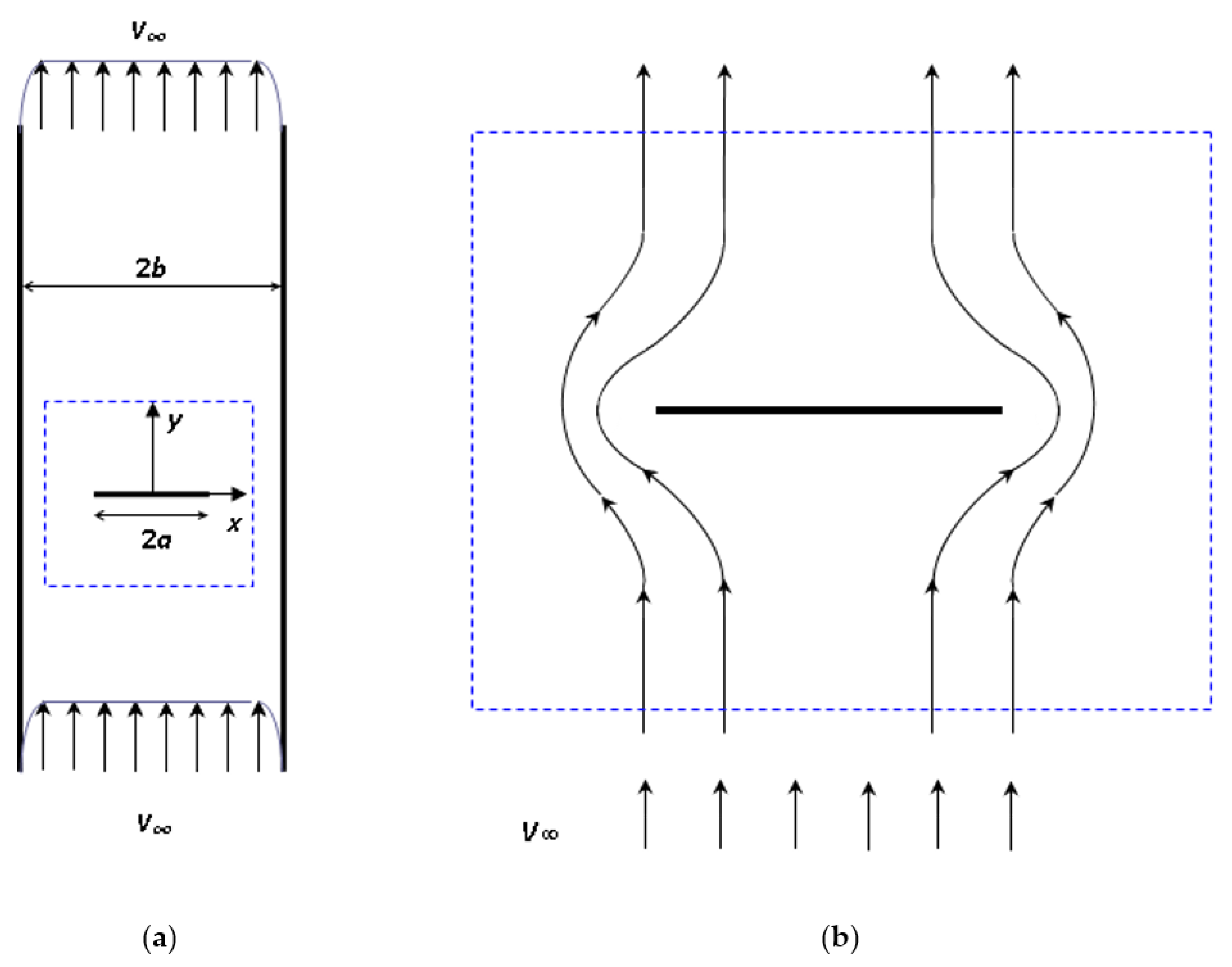
Let us consider a plane flow past a transversal thin plate installed in a straight channel (Figure 2a). The fluid domain is represented by the strip $-b<x<b$ between the channel walls at $x=\pm b$, excluding a segment $-a<x<a$, for $y=0$, occupied by the extremely thin transversal plate. The fluid flows in the positive $y$-direction with inlet velocity $v_{\infty }$.

The complex potential associated with the external flow around the plate is found to be [19]

$$Z=-\mathrm{i}{v}_{\infty }\sqrt{z^2-a^2}$$

(5)

The boundary condition at the surface of the plate is stated as an impenetrability condition:

$$v·n=v_y=0 \mathrm{for} y=0,-a<x<a$$

(6)

where $e_y=n$ is the unit vector normal to the plate surface.

Let us recall that the no-slip condition for fluid layers adherent to the plate, $v=0$, cannot be applied, since the complex potential theory treats the flow as inviscid, i.e., frictionless.

At large distances from the plate, the flow must be asymptotic to the uniform stream. Hence,

$$v_x=0, v_y=v_{\infty } \mathrm{for} \left|z\right|\to \infty$$

(7)

The complex conjugate velocity

$$Z^{\prime }=-\frac{\mathrm{i}{v}_{\infty }z}{{\left(z^2-a^2\right)}^{1/2}}$$

(8)

fulfills the boundary condition (6), since $Z^{\prime }$ is real for $y=0$ and $-a<x<a$, and therefore,$v_y=-$Im$Z^{\prime }$ vanishes. The boundary condition at infinity (7) is met as well, being $Z^{\prime }\cong$ $-\mathrm{i}{v}_{\infty }$, and then $v_x=$ Re$Z^{\prime }=0$, $v_y=-$Im$Z^{\prime }=v_{\infty }$ for $\left|z\right|\gg a$. Therefore, Equation (5) is really the complex potential associated with the flow field shown in Figure 2b.

Function $Z^{\prime }$ in Equation (8) is singular at $z=\pm a$, leading to unbounded flow velocities at both plate extremities. Therefore, the study of the velocity field in the extreme vicinity becomes very important, since it may be related to vortex shedding in the wake behind the plate.

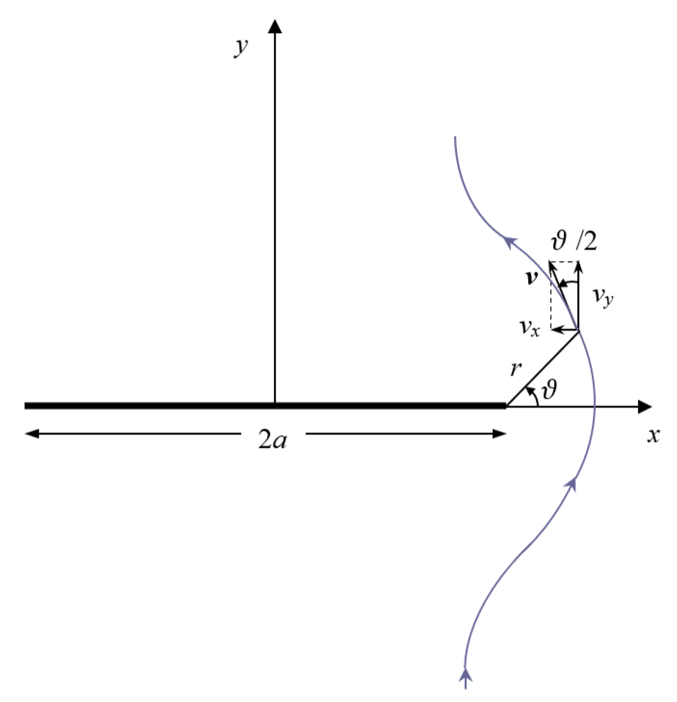
By placing the origin of the coordinate system at the plate edge $z=a$ through the transformation $\zeta =z-a$, Equation (8) takes the form

$$Z^{\prime }=-\frac{\mathrm{i}{v}_{\infty }\left(\zeta +a\right)}{{\left[\zeta \left(\zeta +2a\right)\right]}^{1/2}}$$

(9)

The flow field near the edge is obtained from the limit expression of $Z^{\prime }$ as $\left|\zeta \right|\to 0$

$$Z^{\prime }=-\frac{\mathrm{i}K }{\sqrt{2\pi \zeta }}$$

(10)

where

$$K=v_{\infty }\sqrt{\mathsf{\pi }a}$$

(11)

Using polar coordinates, $\zeta =r{\mathrm{e}}^{\mathrm{i}\vartheta }$, the near-edge solution (10) can be written as

$$Z^{\prime }=\frac{K }{\sqrt{2\pi r}}\left(-\sin \frac{\vartheta }{2}-\mathrm{i}\cos \frac{\vartheta }{2}\right)$$

(12)

Then, the velocity components (Figure 3) exhibit the expected $r^{-1/2}$ singularity at sharp edges [20,21]:

$$v_x=\mathrm{Re} Z^{\prime }=-\frac{K }{\sqrt{2\pi r}}\sin \frac{\vartheta }{2}$$

(13a)

$$v_y=-\mathrm{Im} Z^{\prime }=\frac{K }{\sqrt{2\pi r}}\cos \frac{\vartheta }{2}$$

(13b)

3. Turbulent-to-Vortex-Shedding Fluid-Flow Transition

The continuity equation for incompressible flows imposes the deviation of streamlines around the impenetrable plate, which results in a velocity intensification at the extremities. Hence, the velocity-intensity factor, $K$, is a likely candidate to rule the local turbulent-to-vortex-shedding transition. It is worth noting that the velocity-intensity factor (Equation (11)) presents the following physical dimensions: [K] = [L]^3/2 [T]⁻¹, which are intermediate between those of a velocity, [$v$] = [L] [T]⁻¹, and a kinematic viscosity, [μ] = [L]² [T]⁻¹.

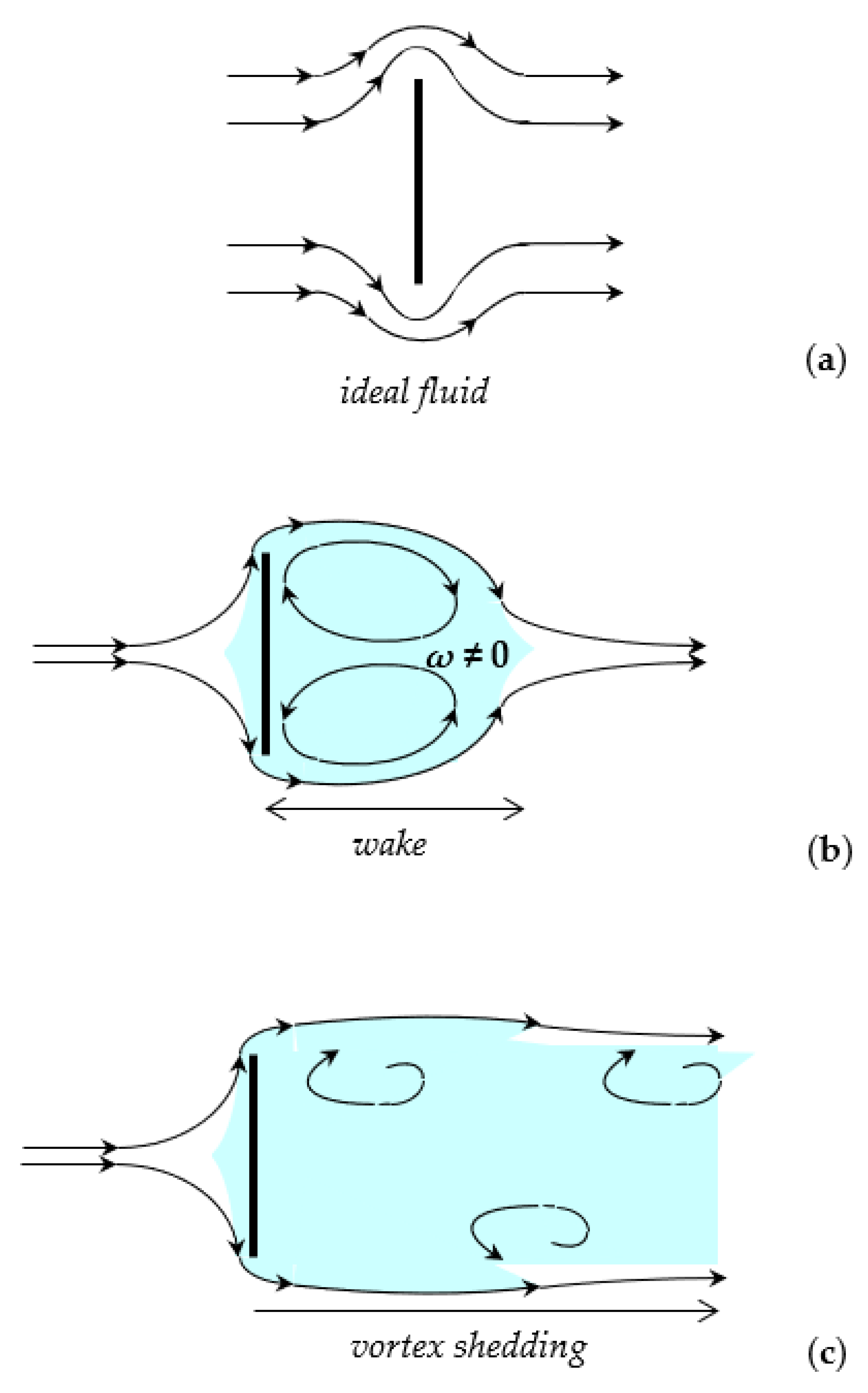
Noticeably, the inviscid flow solution (Equation (5)) is found to be symmetrical upstream and downstream with respect to the plate (Figure 4a), whereas, as a viscosity effect, the real fluid is no longer able to follow the plate’s contour, resulting in an asymmetric flow pattern featured by large-scale eddies downstream from the plate: this region of eddying motion is usually known as the wake. However, the singularity r^−1/2 and the amplifying factor $K$ of the near-edge field are expected to be still valid for real fluids.

When the values of $K$ are sufficiently small, the inertial forces are negligible and the streamlines converge behind the plate. However, the boundary layer separates symmetrically from both sides of the plate, and two eddies are formed, which rotate in opposite directions and remain unchanged in position. In the current condition, the length of the wake is limited. Behind it, the main streamlines converge as depicted in Figure 4b.

Above a certain critical value, $K=K_C$, the arrangement becomes unstable: vortex shedding is expected to take place, where vortices are created at the back of the plate and detach periodically from either side, thereby forming the so-called von Karman vortex street illustrated in Figure 4c.

The critical value $K_C$ would denote a fluid property to be determined by specific experiments and could be identified as shedding toughness, which is analogous to the well-known fracture toughness for solids. Based on Equation (11), the inlet flow velocity $v_{\infty }^{cr}$ for the onset of vortex shedding is predictable by a Griffith-like criterion:

$$v_{\infty }^{cr}=\frac{K_C}{\sqrt{\pi a}}$$

(14)

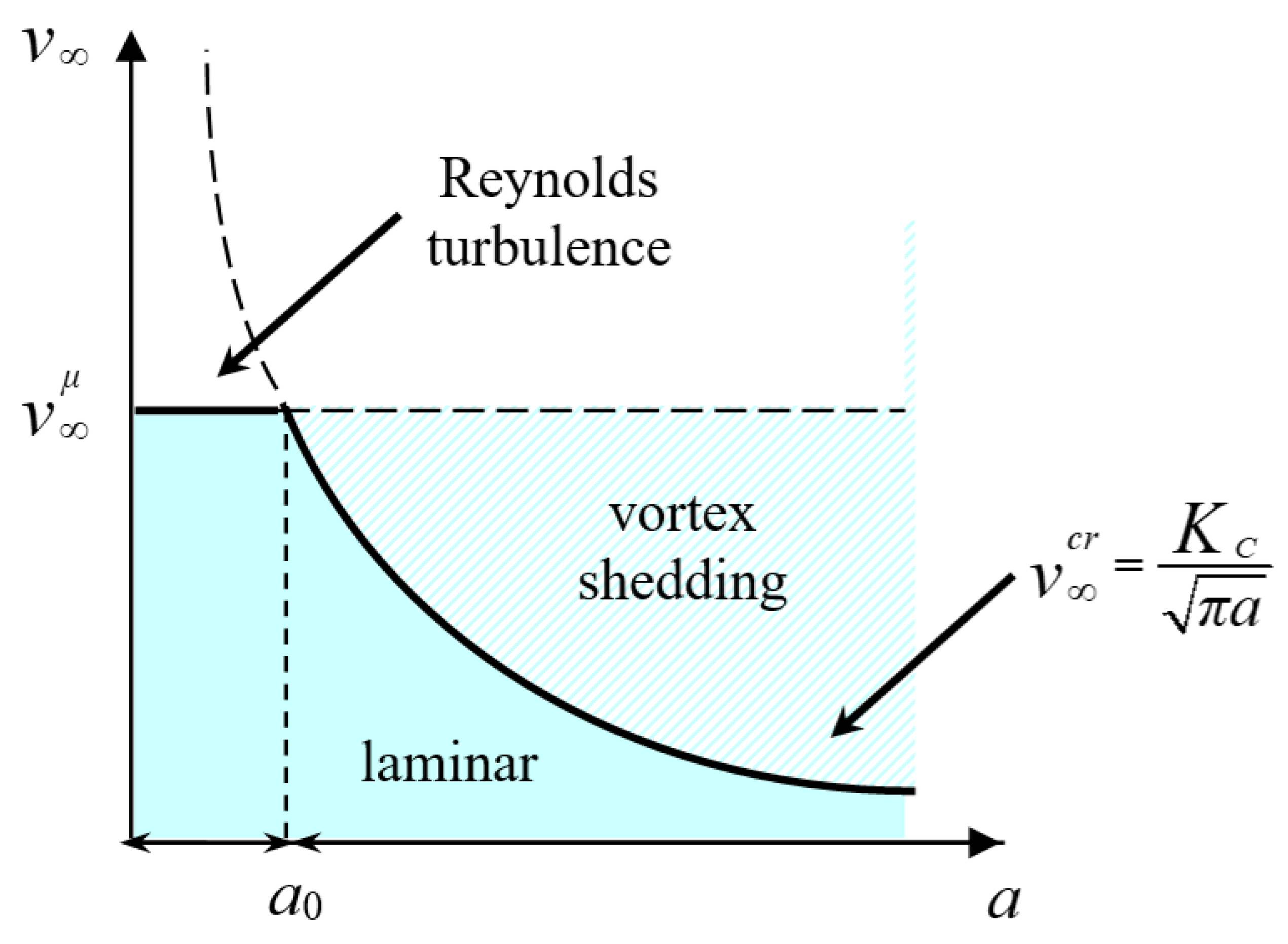
In other terms, the critical velocity $v_{\infty }^{cr}$ required to force the transition to vortex shedding at low Reynolds numbers, $Re<R{e}_C$, i.e., in nominally laminar flows, is inversely proportional to the square root of the plate half-width, $v_{\infty }^{cr}\propto a^{-1/2}$. In reality, such behavior would be unphysical, since turbulence starts to develop naturally when the critical Reynolds number $R{e}_C$ is reached.

The variation in the critical velocity versus plate width is illustrated in Figure 5 by the solid curve, that separates laminar from turbulent flow conditions in the domain ($a, v_{\infty }$). The horizontal straight line represents the critical velocity $v_{\infty }^{\mu }$ for the onset of Reynolds turbulence:

$$v_{\infty }^{\mu }=\frac{R{e}_C\mu }{D}$$

(15)

where $\mu$ is the kinematic viscosity and $D=2b$ is the channel width.

The intersection of the curves given by Equations (14) and (15) defines a transition length:

$$a_0=\frac{1}{\pi }{\left(\frac{K_{C}D}{\mu R{e}_C}\right)}^2$$

(16)

ruling out the competition between Reynolds turbulence and vortex shedding.

For $a<a_0$, when the $v_{\infty }^{cr}$ curve overcomes the horizontal line $v_{\infty }^{\mu }$, Reynolds turbulence precedes vortex shedding behind the plate. As a matter of fact, the flow does not sense plates of size smaller than $a_0$, and only Reynolds turbulence is possible. The limit plate size $a_0$ that a laminar flow can sustain safely represents the obstacle sensitivity, i.e., the smaller is $a_0$, the more obstacle-sensitive is the flow. Thus, the flow is sensitive to the presence of plates with $a>a_0$, which can drive the transition to vortex shedding at critical velocities $v_{\infty }^{cr}$lower than $v_{\infty }^{\mu }$, i.e., for Reynolds numbers $Re$ lower than $R{e}_C$.

From Equation (16), we can see that a decrease in the channel width, D, provides a decrease in the limit value $a_0$. Namely, bringing the channel walls closer to the plate enhances the vortex formation and shedding behind the plate, whereas the Reynolds turbulence tends to anticipating the vortex shedding if the channel is sufficiently wide. This confinement effect seems to be analogous to the wall effect, as reported in numerical studies on the flow past a bluff body installed in a channel [17,22,23]. Those investigations show that reduced separation between the body and the channel wall facilitates the appearance of twin vortices in the wake.

It can be said that the scale effect highlighted by Equation (16) is due to the mismatch between two fluid properties with different physical dimensions: the kinematic viscosity, $\left[\mu \right]={\left[L\right]}^2{\left[T\right]}^{-1}$, and the shedding toughness, $\left[K_C\right]={\left[L\right]}^{3/2}{\left[T\right]}^{-1}$. A strong analogy with fracture mechanics exists, where scale effects in fracture testing are mainly due to the co-existence of two generalized forces with different physical dimensions: the stress, $\left[\sigma \right]=\left[F\right]{\left[L\right]}^{-2}$, and the stress-intensity factor, $\left[K\right]=\left[F\right]{\left[L\right]}^{-3/2}$ [5,7].

4. Effect of the Channel Width

The complex potential of Equation (5) is associated with an unbounded flow velocity around the plate edge, implying that channel walls are supposed to be far enough from the plate not to affect the flow around it. Namely, confinement effects have been so far considered solely via the Reynolds number. As a matter of fact, when the channel shrinks or when the plate size increases, the walls exert an enhanced influence on the flow field near the plate edges. In such a case, some corrections to the flow solution may be properly introduced.

The wall proximity effect due to the channel width can be considered by including a shape factor $Y$ in the $K$ solution:

$$K=Y{v}_{\infty }\sqrt{\mathsf{\pi }a}$$

(17)

such that $K$ approaches the value of Equation (12) as $a/b\to 0$, i.e., for a channel width much larger than the plate width, and it diverges as $a/b\to 1$.

The shape factor $Y$ is a dimensionless function of the $a/b$ ratio that can be obtained by numerical investigations.

Equation (17) can be expressed in the form

$$K=v_{\infty }\sqrt{2\mathrm{b} }f\left(a/b\right)$$

(18)

where $f\left(\frac{a}{b}\right)={\left(\frac{\pi a}{2b}\right)}^{1/2}Y$.

Equation (18) provides a critical inlet velocity to force the transition to vortex shedding, where the wall effects are explicitly taken into account:

$$v_{\infty }^{cr}=\frac{K_C}{f\left(a/b\right) \sqrt{2b}}$$

(19)

By exploiting Equation (15), Equation (19) takes a dimensionless form:

$$\frac{v_{\infty }^{cr}}{v_{\infty }^{\mu }}=\frac{s}{f\left(a/b\right) }$$

(20)

where the dimensionless number

$$s= \frac{K_C{b}^{1/2}}{\mu }$$

(21)

can be called the shedding number, in full analogy with the brittleness number that governs the ductile-to-brittle transition in elastic–plastic cracked bodies [5,22]. In this case, two different failure modes are possible: (i) plastic collapse of the solid, when the strength of the material, τ_P, is overcome and the crack is considered as a weakening of the body’s cross-section without including any local effect; (ii) crack propagation determined by the achievement of the fracture toughness, K_IIIC, of the material. For the brittleness number, $s=\frac{K_{\mathrm{III}C}}{{\tau }_{\mathrm{P} }{b}^{1/2}}$, both the mechanical properties of the material and the characteristic size of the solid are relevant. It is possible to demonstrate that brittle failure occurs only with relatively low fracture toughness values, high material strengths, and/or large structural sizes [5,23].

On the other hand, by considering the shedding number (Equation (21)), a reverse scale effect becomes manifest: vortex shedding occurs only with relatively low shedding toughness values, high kinematic viscosities, and/or small channel widths.

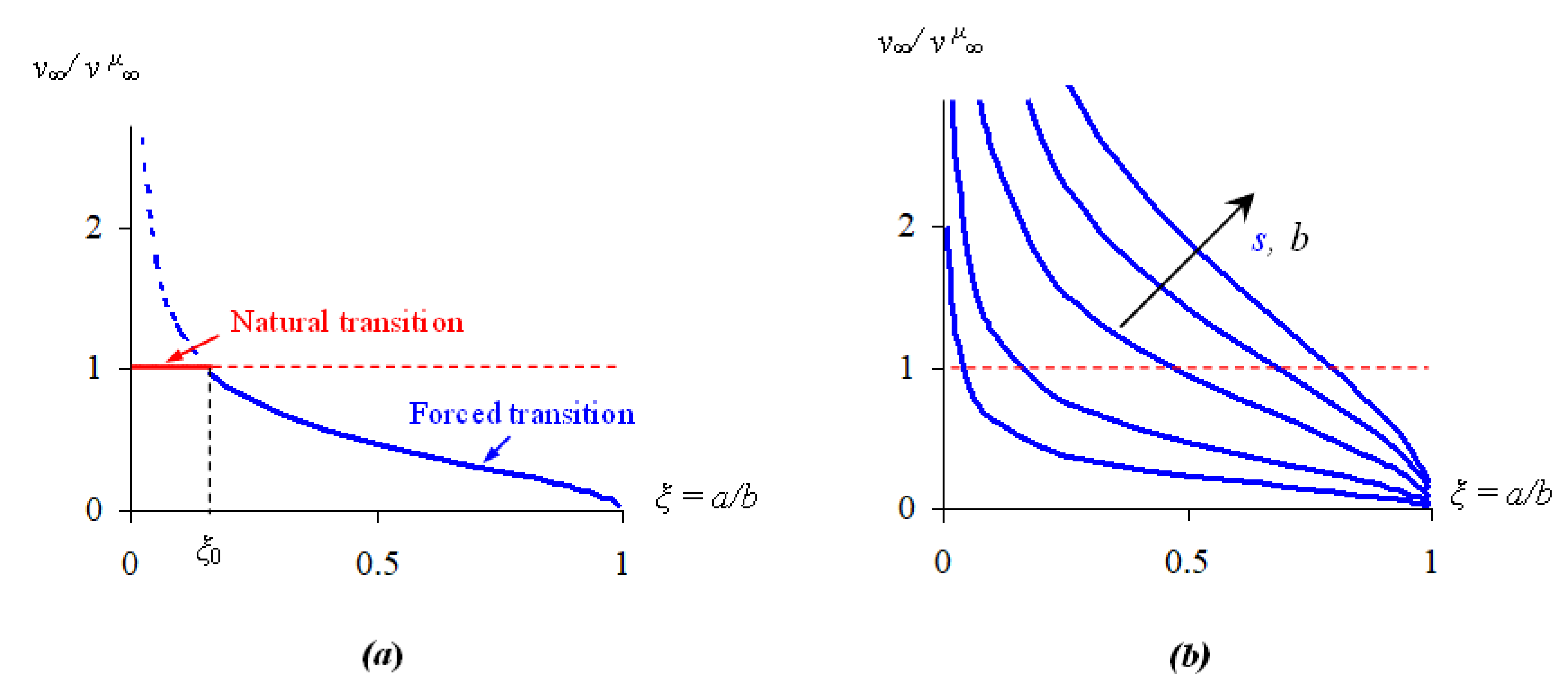
The competition between natural and forced (turbulent to vortex shedding) transitions is investigated as a function of the blockage ratio, $\xi =a/b$. The condition for vortex shedding is represented by a set of curves in the $\left(\xi ,\upsilon \right)$ diagram―$v=v_{\infty }/v_{\infty }^{\mu }$ being the normalized inlet velocity―by varying the shedding number $s$ in Equation (20), whereas the condition for Reynolds turbulence is represented by a single horizontal straight line $v=1$ (see Figure 6).

These curves separate distinct regions, each corresponding to a different flow regime. It is evident that vortex shedding occurs only for blockage ratios above the limit value ξ₀ (see Figure 6a).

As is shown in Figure 6b, the diverging vortex-shedding curves overcome the horizontal line $\upsilon =1$ for most blockage ratios $\xi =a/b$, when $s$ is sufficiently high. This means that the Reynolds turbulence tends to anticipate and obscure the vortex shedding even for high $a/b$ ratios, if the channel width $b$ is sufficiently large.

This scale effect is also revealed by the quadratic scaling of the obstacle sensitivity (Equation (16)) with the channel width, $a_0\propto b^2$, whereby for fixed ratios $a/b$ and by increasing $b$, the Reynolds turbulence tends to become the dominating mechanism [22,24].

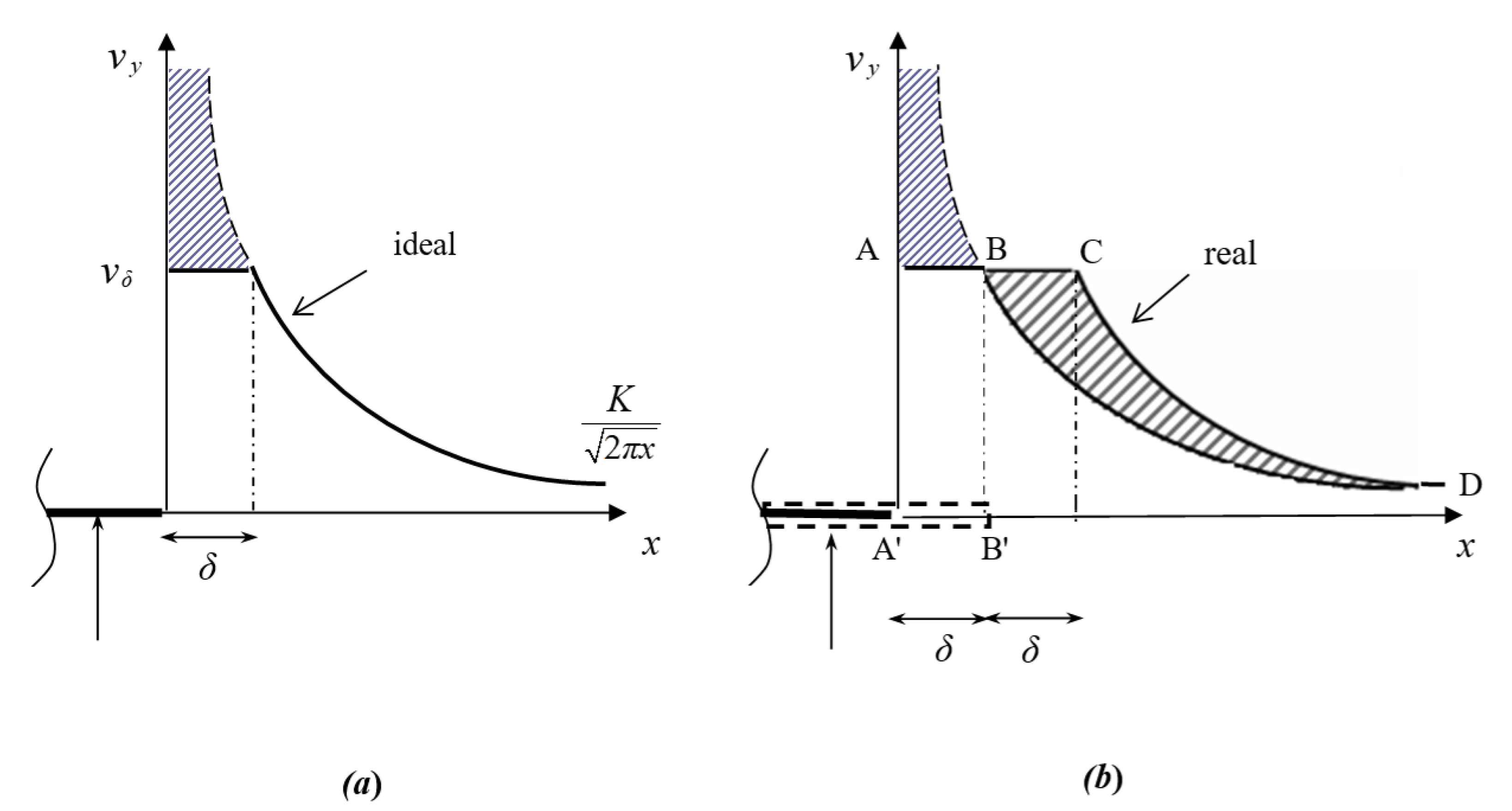
5. Viscosity at the Edges of the Obstacle

Considering real fluids, potential flow solutions must take into account the effects of viscosity within the boundary layer, where a velocity profile develops and truncates the singularity near sharp edges [25]. This is analogous to considering, in the framework of fracture mechanics, the plastic phenomena occurring at small distances from the crack tip, which relieve the elastic singularity. Hence, the concept of plastic-zone extension resembles that of boundary-layer thickness [26], defined as the distance of the solid surface to the boundary between viscous flow and external flow. An alternative parameter is the boundary layer displacement, $\delta$, which is defined as the distance at which the potential flow has to translate to produce the same mass flow rate as the real fluid [27,28]. Due to the slowing down of the real fluid in the boundary layer, this ideal flow essentially encounters an effective obstacle larger by $\delta$, namely, an extended fictitious plate with $a_{e\mathrm{ff}}=a+\delta$.

Hereafter, an Irwin-like approach [29] is proposed to estimate the critical boundary-layer thickness ahead of the edge of the plate. The singular velocity distribution $v_y\left(\vartheta =0\right)$ given by Equation (13b) is truncated by viscosity, and a flat profile $v_y=v_{\delta }$ for $x\le \delta$ is simply assumed (Figure 7a). Consequently, the condition $v_y=v_{\delta }=K/{\left(2\pi \delta \right)}^{1/2}$ gives the first approximation of the boundary layer’s thickness.

$$\delta =\frac{1}{2\pi }{\left(\frac{K}{v_{\delta }}\right)}^2$$

(22)

This estimate is not strictly correct because the conservation of mass rate appears to be violated. When the effect of viscosity is considered, velocities must redistribute in order to satisfy the conservation of mass rate. Namely, the singular velocity distribution is translated along the x-axis, so that the integral of the redistributed velocities (curve ABCD in Figure 7b) is equal to the integral of the aforementioned singular distribution. The integral of $v_y$ between the plate edge and the point $x=\delta$ gives

$${{\displaystyle \int }}_0^{\delta }K\mathrm{d}x/\sqrt{2\pi x}=2\delta v_{\delta }$$

(23)

where Equation (22) is exploited.

Therefore, the left-hand hatched area of Figure 7b is $\delta v_{\delta }$. Additionally, the right-hand hatched area, obtained with a translation by $\delta$, is equal to that of the rectangle A’ABB’, since both of them are complementary to the area underneath the curve BD, so that the conservation of mass is satisfied. Thus, a more accurate evaluation of the thickness of the boundary layer is $\tilde{\delta }=2\delta$. Finally, we obtain the following expression for the thickness of the boundary layer when vortex shedding starts:

$${\tilde{\delta }}_C=\frac{1}{\pi }{\left(\frac{K_C}{v_{\delta }}\right)}^2$$

(24)

Furthermore, if it is assumed $v_{\delta }=v_{\infty }^{\mu }$, ${\tilde{\delta }}_C$ comes to coincide with the obstacle sensitivity $a_0$ (see Equation (16)):

$${\tilde{\delta }}_C=a_0=\frac{1}{\pi }{\left(\frac{K_{C}D}{\mu R{e}_C}\right)}^2$$

(25)

This correspondence is analogous to that emerging in fracture mechanics between the size of the characteristic microcrack for the material and the size of the plastic zone at crack propagation [30].

Finally, considering the two problems represented in Figure 1, the aforementioned analogies are summarized in

Table 1. Summary of the main analogies.

Linear elastic constitutive laws: $\begin{array}{c}{\tau }_{xz}=G\frac{\partial w}{\partial x }\\ {\tau }_{yz}=G\frac{\partial w}{\partial y }\end{array}$ w= displacement along the z-axis	Potential flow (outside boundary layers and wakes): $\begin{array}{c}{v}_x=\frac{\partial \phi }{\partial x}\\ v_y=\frac{\partial \phi }{\partial y}\end{array}$ φ = velocity potential
Indefinite equilibrium equation: $\frac{\partial {\tau }_{xz}}{\partial x }+\frac{\partial {\tau }_{yz}}{\partial y }=0$	Continuity equation: $\frac{\partial v_x}{\partial x }+\frac{\partial v_y}{\partial y }=0$
Combining the above equations gives: ${\nabla }^{2}w=0\Rightarrow w=$Im$Z_{\mathrm{III}}/\mu$ where $Z_{\mathrm{III}}$ is an analytic function From the constitutive laws, it follows: ${\tau }_{xz}=$ Im$Z_{\mathrm{III}}^{\prime }$ ${\tau }_{yz}=$ Re$Z_{\mathrm{III}}^{\prime }$	Combining the above equations gives: ${\nabla }^2\phi =0\Rightarrow \phi =$Re$Z$ where $Z$ is an analytic function From the velocity potential, it follows: $v_x=$ Re$Z^{\prime }$ $v_y=-$Im$Z^{\prime }$
Boundary conditions: Stress-free crack surfaces: ${\tau }_{yz}=0\hspace{1em}$ for $y=0$, $-a<x<a$ Boundary conditions at infinity: ${\tau }_{xz}=0$, ${\tau }_{yz}=\tau \hspace{1em}$ for $\left|z\right|\to \infty$	Boundary conditions: Impenetrable plate surfaces: $v_y=0\hspace{1em}$ for $y=0$, $-a<x<a$ Boundary conditions at infinity: $v_x=0, v_y=v_{\infty }\hspace{1em}$ for $\left|z\right|\to \infty$
Westergaard solution: $Z_{\mathrm{III}}=\tau \sqrt{z^2-a^2} \Rightarrow Z_{\mathrm{III}}^{\prime }=\tau z/{\left(z^2-a^2\right)}^{1/2}$	Complex potential: $Z=-\mathrm{i} v_{\infty }\sqrt{z^2-a^2}$ $\Rightarrow Z^{\prime }=-\mathrm{i} v_{\infty }z/{\left(z^2-a^2\right)}^{1/2}$
Stress field near the crack tip: ${\tau }_{xz}=-\frac{K_{\mathrm{III}} }{\sqrt{2\pi r}}\sin \frac{\vartheta }{2}$ ${\tau }_{yz}=\frac{K_{\mathrm{III}} }{\sqrt{2\pi r}}\cos \frac{\vartheta }{2}$ where $K_{\mathrm{III}}=\tau \sqrt{\pi a}$	Flow field near the plate edge: $v_x=\frac{K }{\sqrt{2\pi r}}\sin \frac{\vartheta }{2}$ $v_y=-\frac{K }{\sqrt{2\pi r}}\cos \frac{\vartheta }{2}$ where $K=v_{\infty }\sqrt{\mathsf{\pi }a}$
Fracture sensitivity: $a_0=K_{\mathrm{III}C}^2/\pi {\tau }_P^2$	Obstacle sensitivity: $a_0=D^2{K}_C^2/\pi {\mu }^{2}R{e}_C{}^2$
Plastic flow collapse: $\tau ={\tau }_{P }$ for $a<a_0$ Crack propagation: $K_{\mathrm{III}}=K_{\mathrm{III}C}$ for $a\ge a_0$	Reynolds turbulence: $Re=R{e}_C$ for $a<a_0$ Vortex shedding: $K=K_C$ for $a\ge a_0$
Size-scale effects of interacting failure modes (${\tau }_{cr}$ = critical applied stress for crack propagation): $\frac{{\tau }_{\mathrm{cr}}}{{\tau }_{\mathrm{P}}}=\frac{s}{g\left(a/b\right)}$ Brittleness number $s=\frac{K_{\mathrm{III}\mathrm{C}}}{{\tau }_{\mathrm{P}} b^{1/2}}$	Size-scale effects of interacting transitional flows ($v_{\infty }^{\mathrm{cr}}$ = critical inlet velocity for vortex shedding): $\frac{v_{\infty }^{\mathrm{cr}}}{v_{\infty }^{\mu }}=\frac{s}{f\left(a/b\right)}$ Shedding number $s=\frac{K_C b^{1/2}}{\mu }$

.

6. Conclusions

The solutions to plane elasticity or to plane fluid-flow problems are often reduced to find the associated complex potentials that satisfy the appropriate boundary conditions. In the framework of the hydrodynamic analogy, calculating the linear elastic stress field associated with Mode III crack loading and the potential flow field past a transversal thin plate represent two equivalent problems.

Furthermore, in both cases, a phase change―either ductile-to-brittle or turbulent-to-vortex-shedding transition―intervenes at a critical point, when a sort of driving force exceeds its critical value.

Failure by general yielding occurs when the applied uniform out-of-plane shearing stress at infinity $\tau$ exceeds the material yield strength ${\tau }_{\mathrm{P}}.$This failure mode is analogous to the laminar-to-turbulent transition of pipe flows, which begins when the Reynolds number $Re$ exceeds its critical value $R{e}_C=2300$. This analogy appears between ${\tau }_{\mathrm{P}}$and the critical inlet velocity, $v_{\infty }^{\mu }=R{e}_C\mu /D$. If the strip or the channel width is fixed, the analogy can be expressed in terms of material or fluid properties, as the ability of the material to sustain applied stresses or the ability of the fluid to sustain laminar flows.

On the other hand, unstable crack propagation from a pre-existing defect occurs when the stress-intensity factor is equal to the Mode III fracture toughness, $K_{\mathrm{III}}=K_{\mathrm{III}C}$. Analogously, vortex shedding is expected to take place in fluid flow when the velocity-intensity factor is equal to the shedding toughness, $K=K_C$, thereby forming the so-called von Karman vortex street. As Mode III fracture toughness, $K_{\mathrm{III}C}$, expresses the ability of the material to resist fracture in the presence of cracks, so the shedding toughness, $K_C$, would express the ability of the fluid to resist generation and shedding of vortices behind obstacles. In addition, as the dimensional mismatch between strength and toughness involves a scale-dependent ductile-to-brittle failure transition in solids, so a scale-dependent turbulent-to-vortex-shedding fluid flow transition is driven by the difference in physical dimensions between the kinematic viscosity and the shedding toughness.

Future research work might concern the experimental measurement of $K_C$, which could be helpful, together with the shedding number $s$, in investigating the competition between different mechanisms in the turbulent-to-vortex-shedding transition. In this framework, it is interesting to recall that, by considering the shedding number, vortex shedding occurs only with relatively low shedding toughness values, high kinematic viscosities, and/or small channel sizes. This scale effect in fluid mechanics turned out to be the reverse of the scale effect that can be detected in solid mechanics by considering the brittleness number: in fact, a truly brittle failure occurs only for relatively low fracture toughness values, high material strengths, and/or large structural sizes.