
Evaluation of Synthetic Jet Flow Control Technique for Modulating Turbulent Jet Noise

Abstract
:1. Introduction
2. Materials and Methods
2.1. Aerodynamic Computation
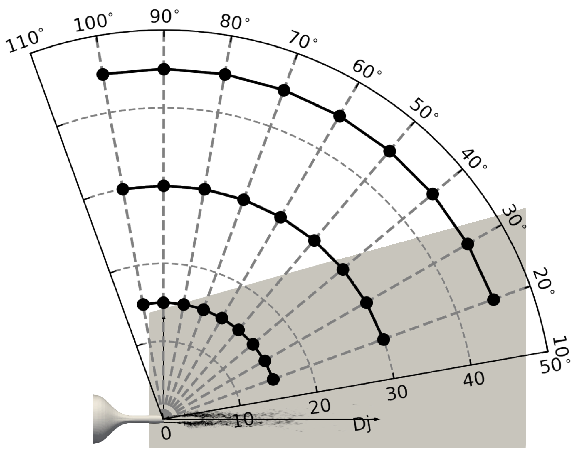
2.2. Aeroacoustic Computation
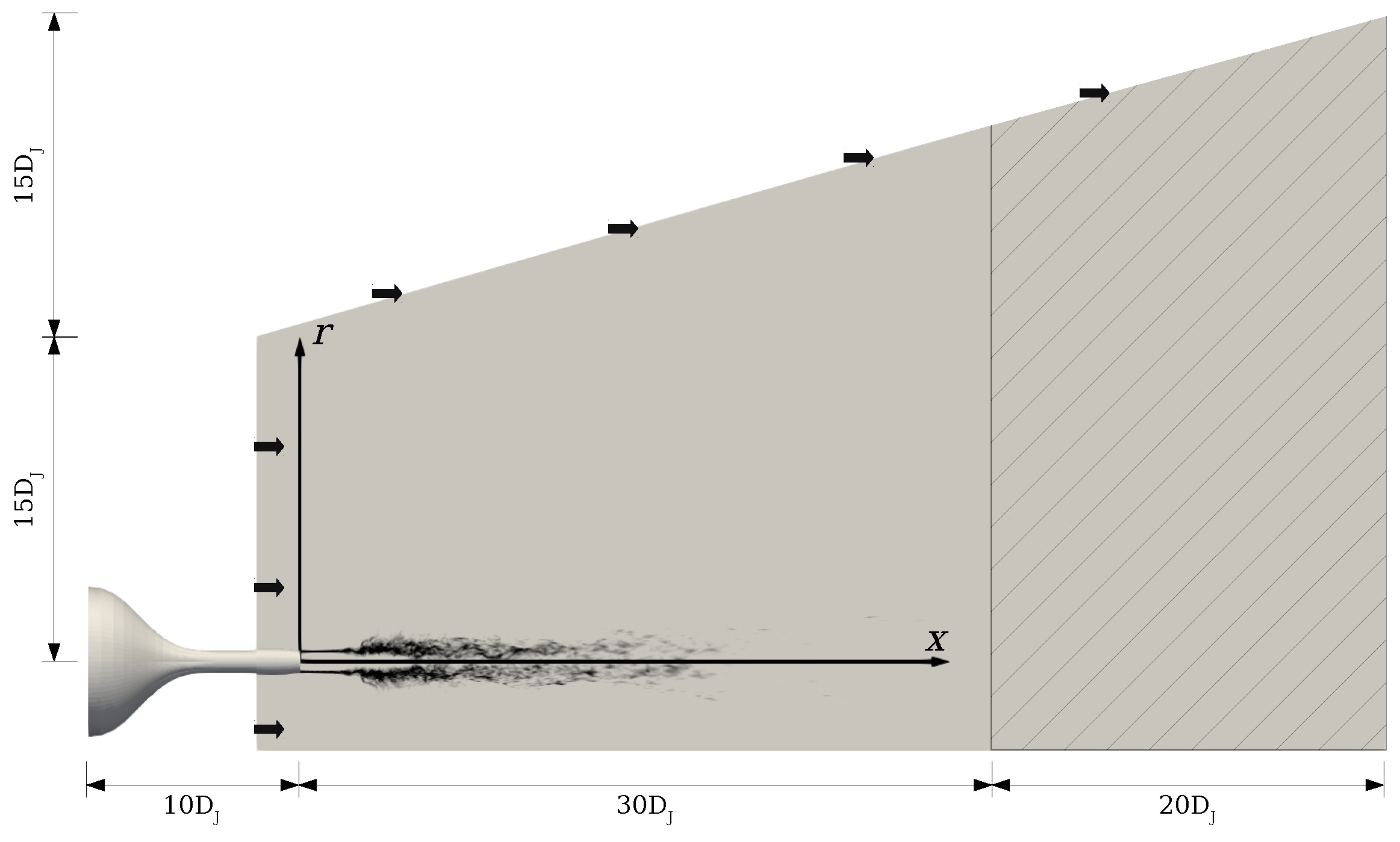
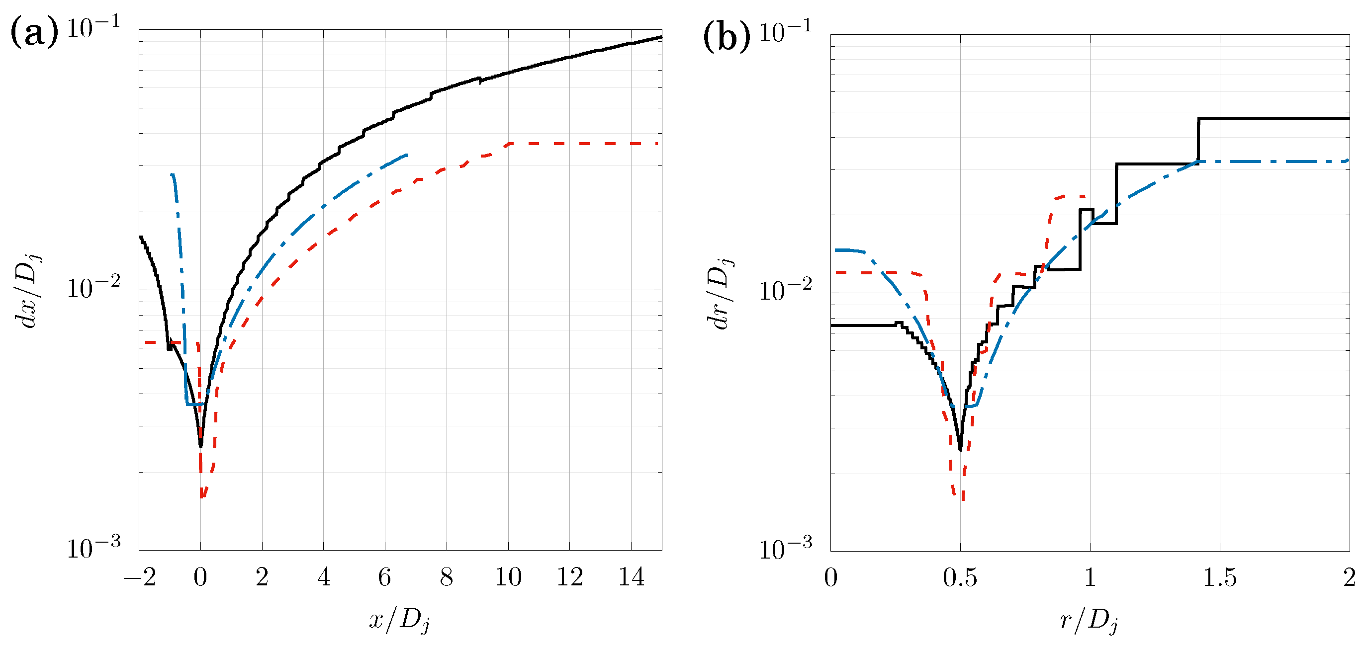
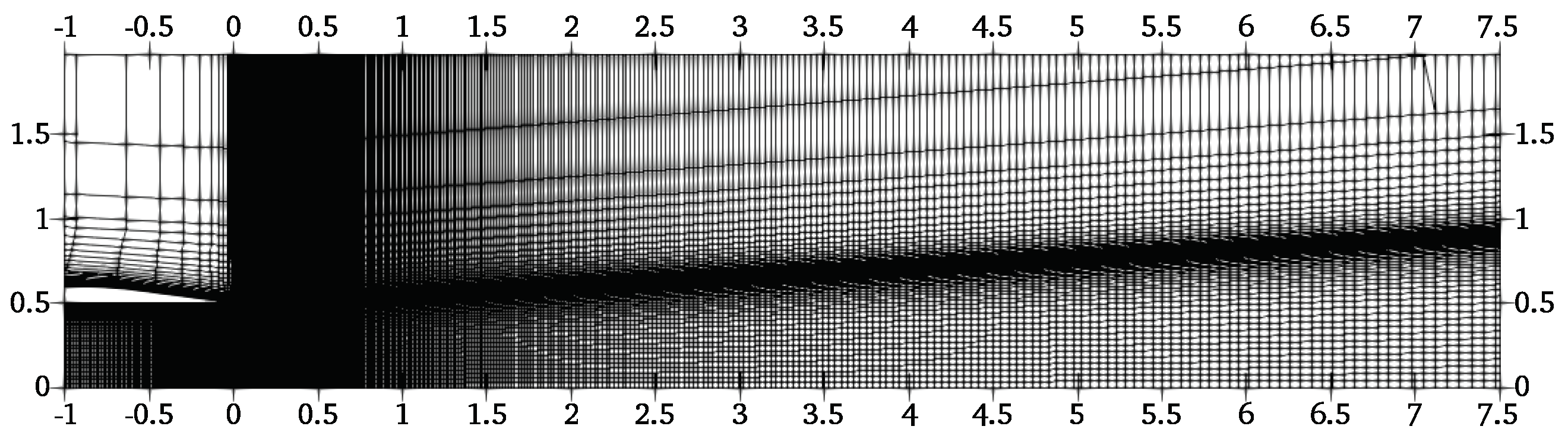
2.3. Computational Model
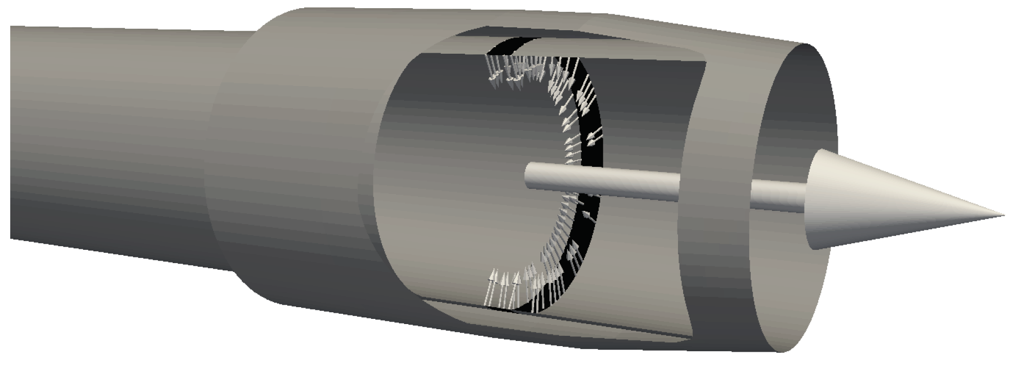
2.4. Flow Control Technique
3. Results and Discussion
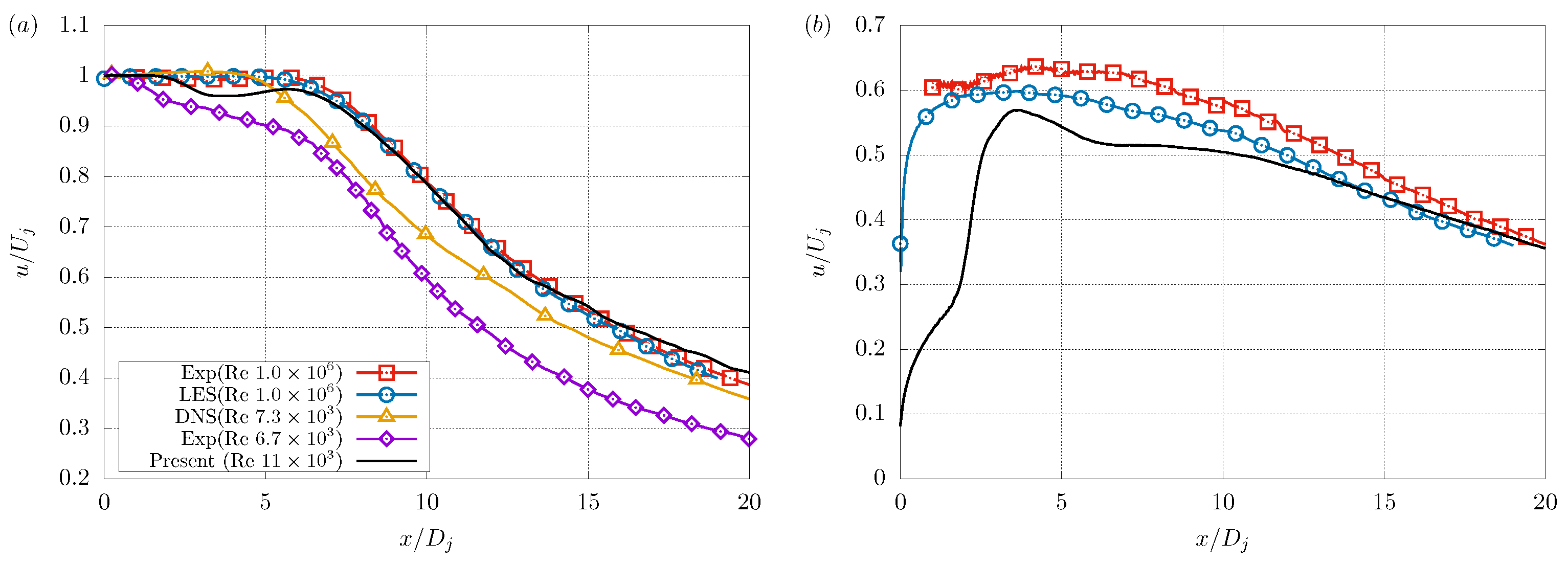
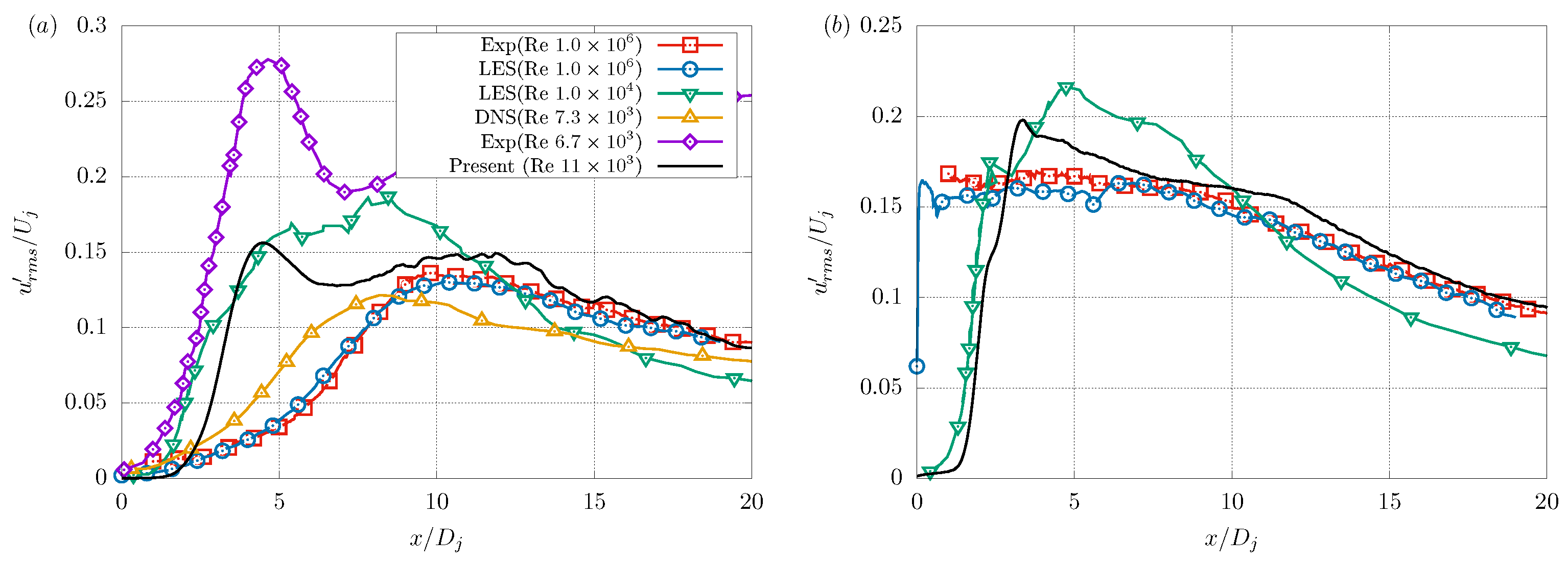
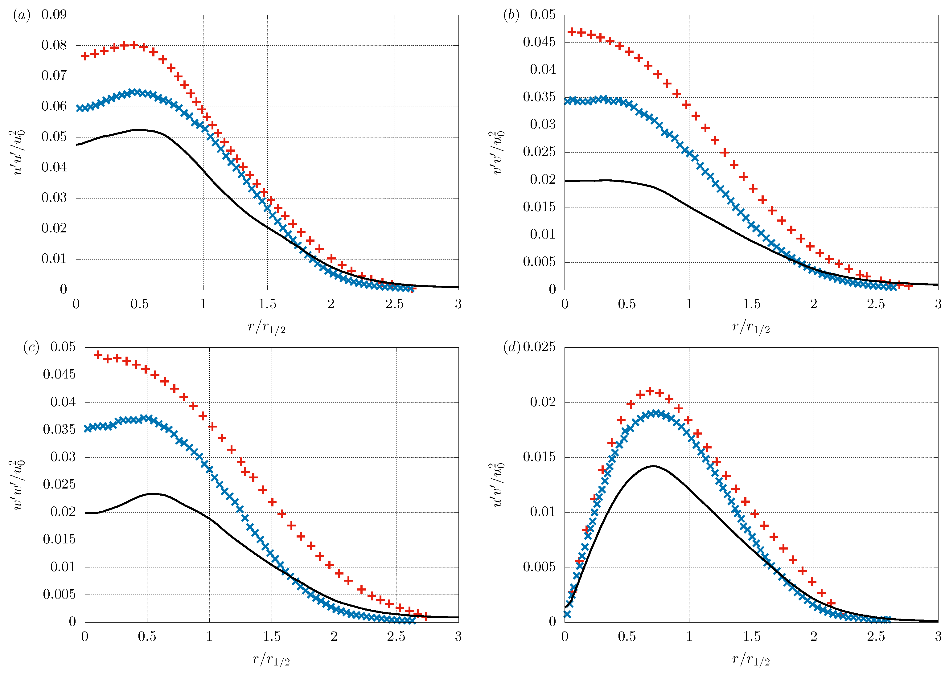
3.1. Validation
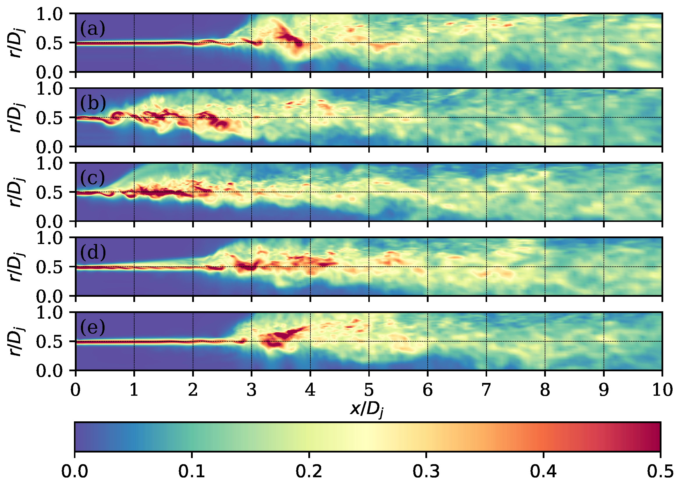
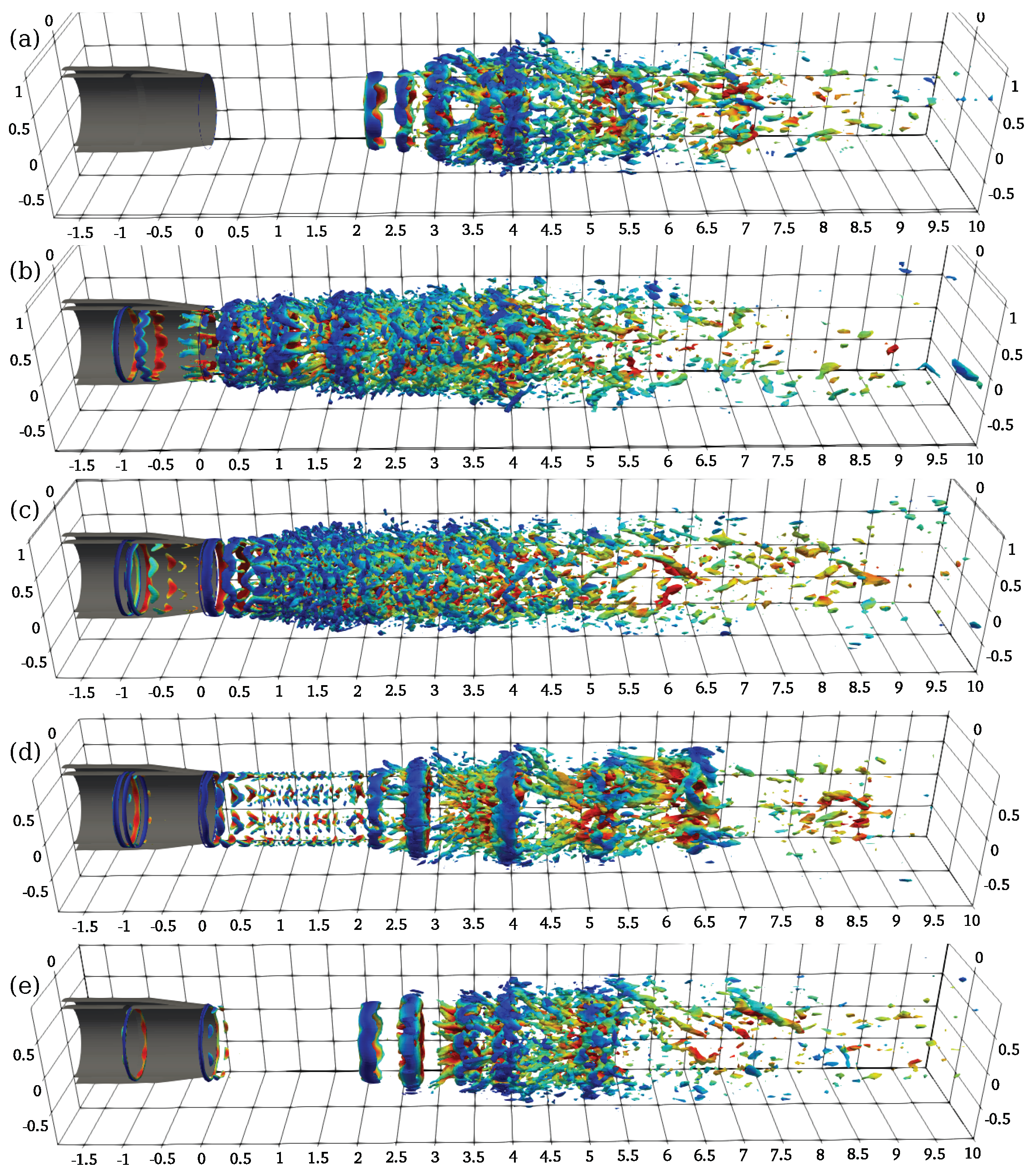
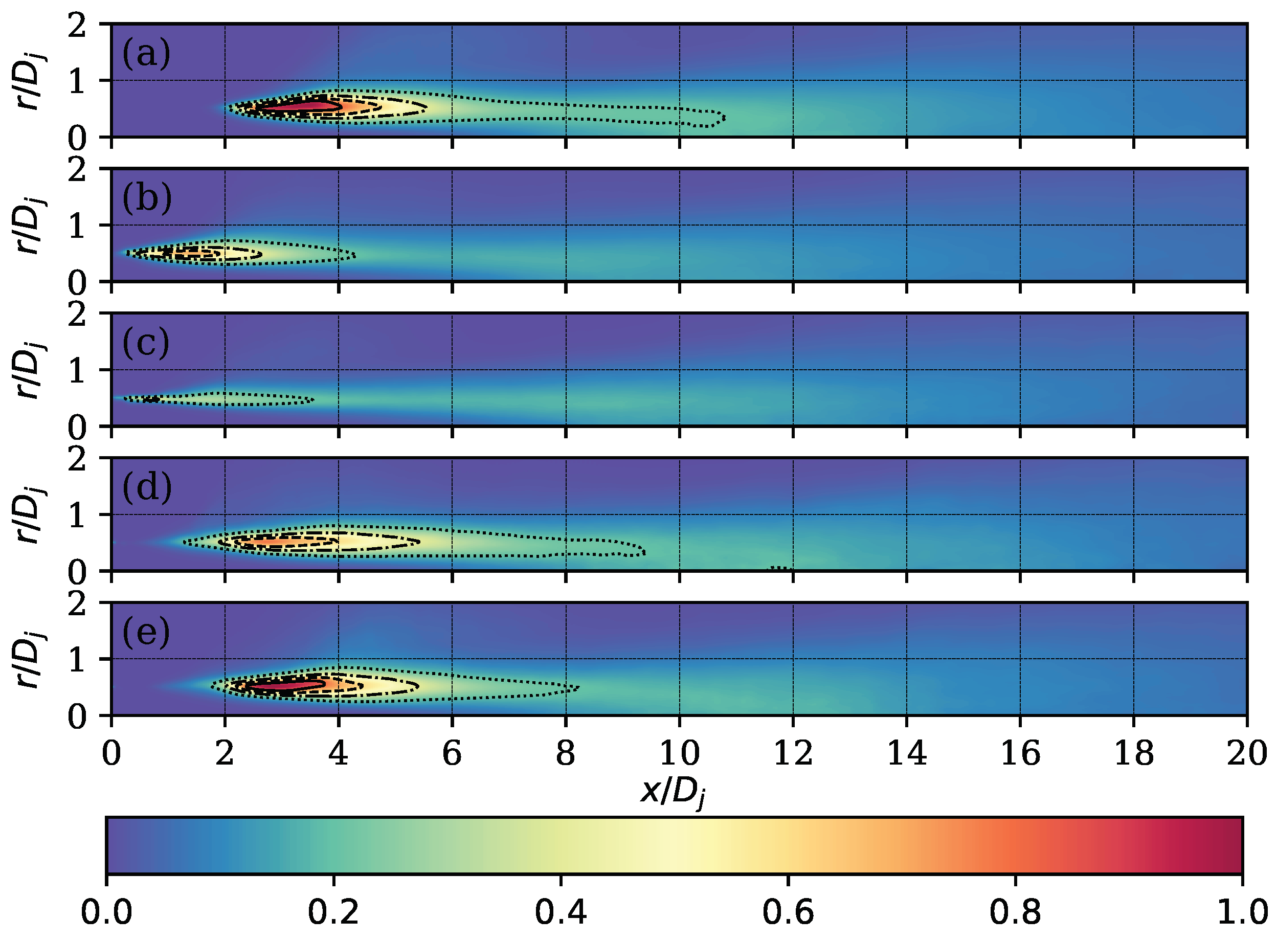
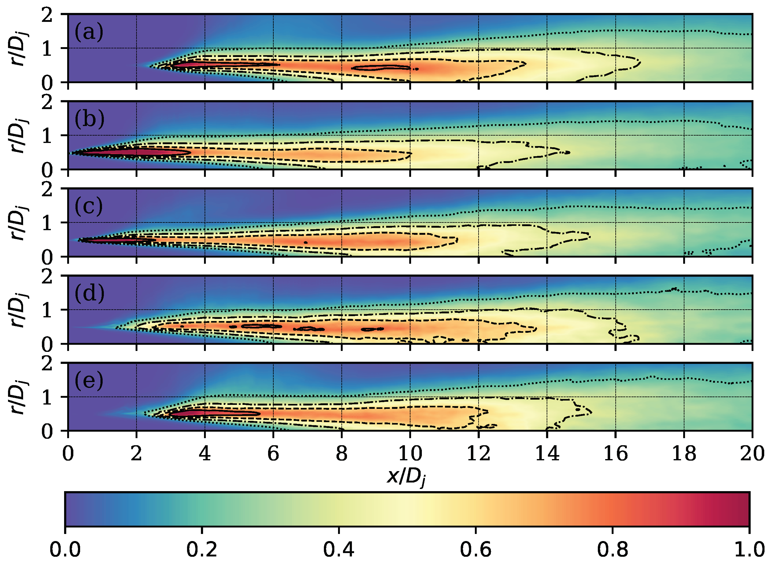
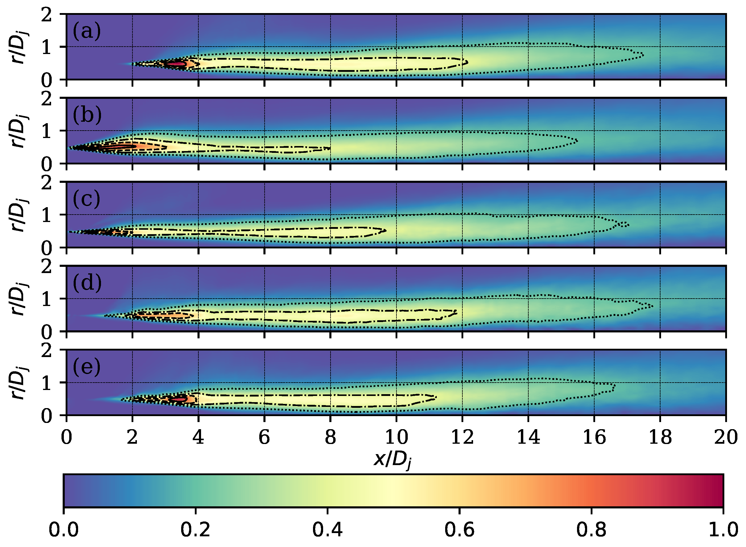
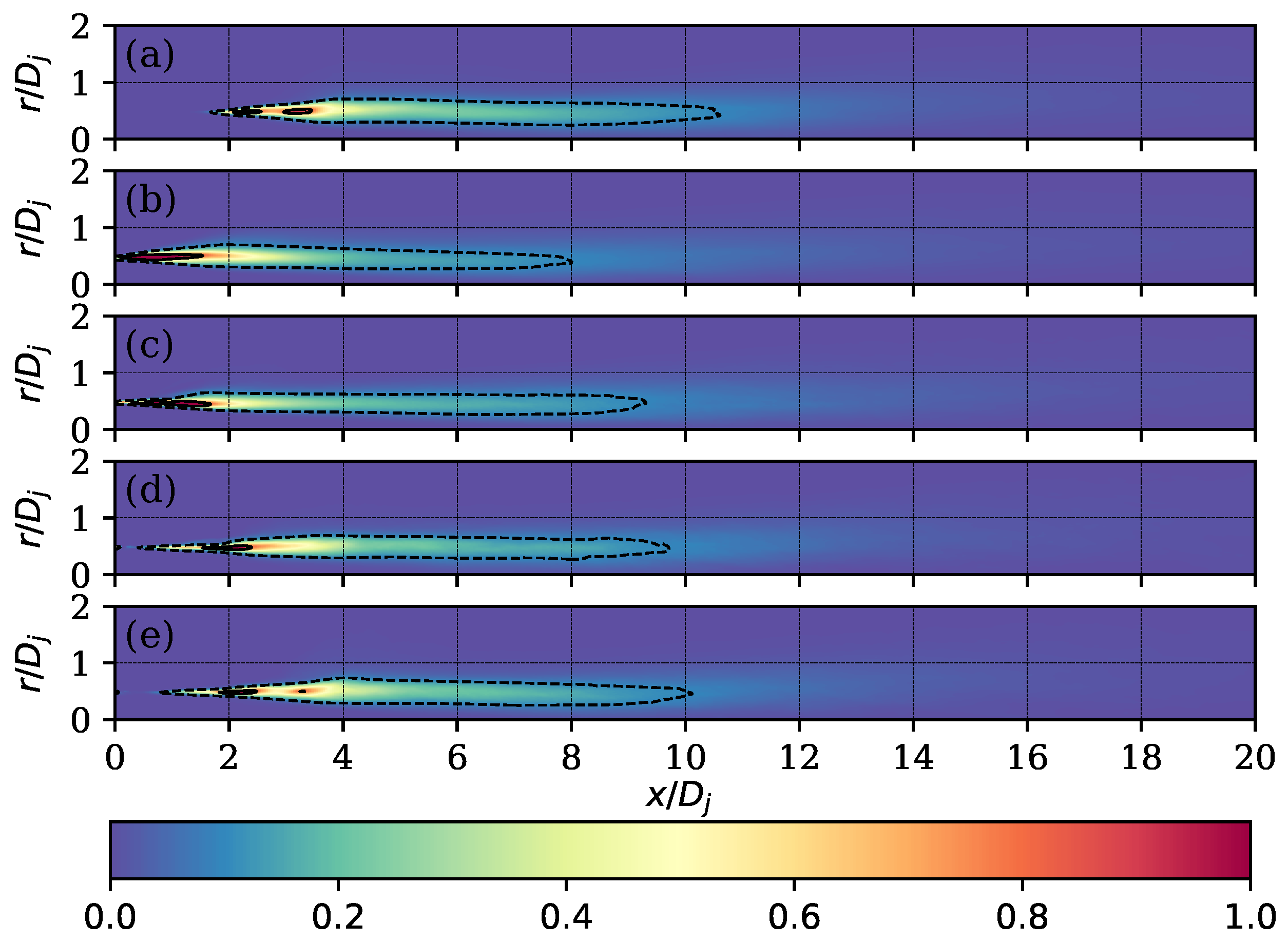
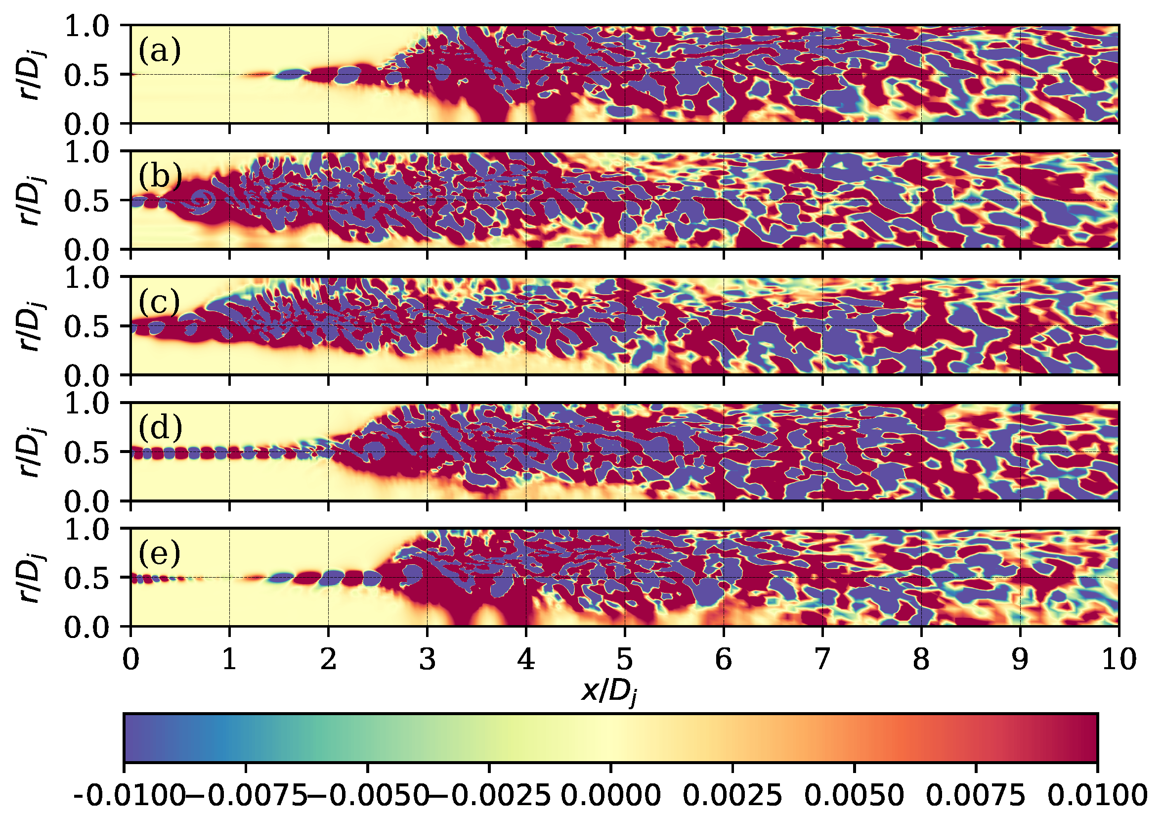
3.2. Flow Field
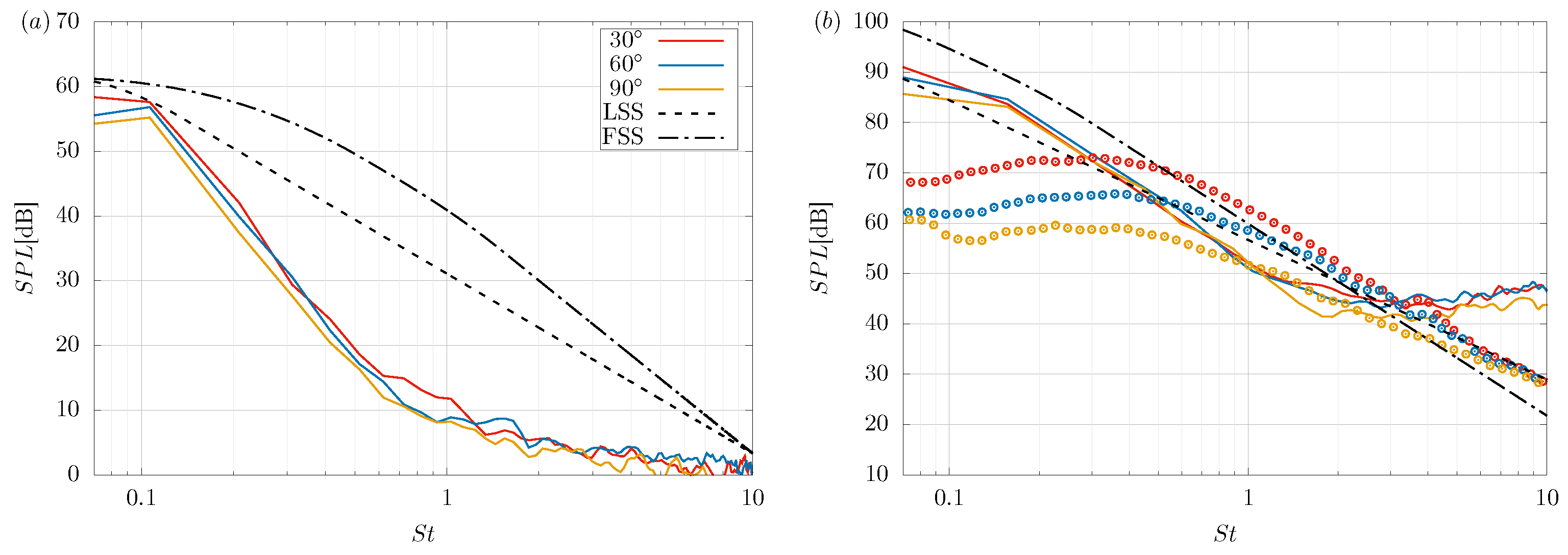
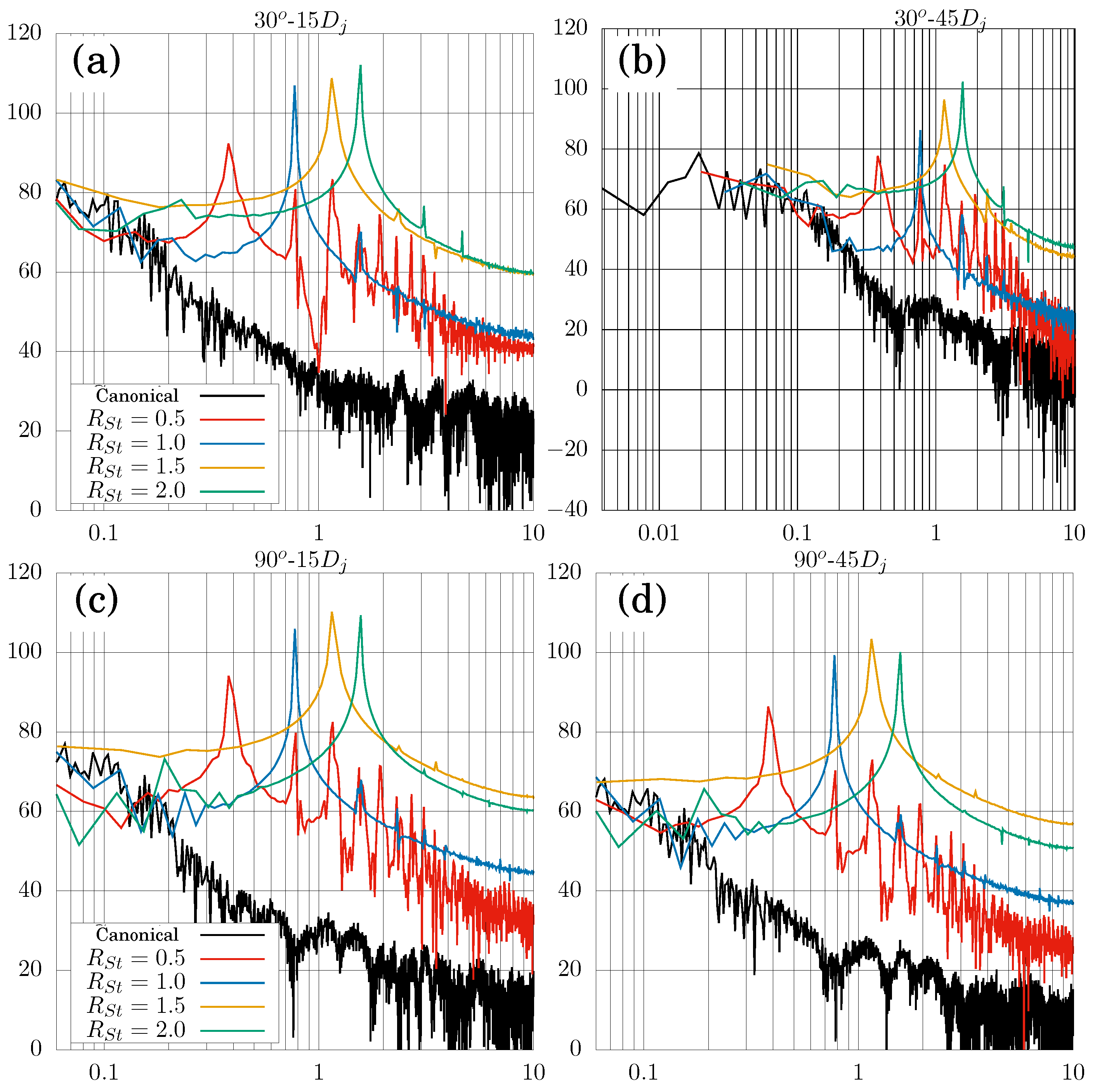
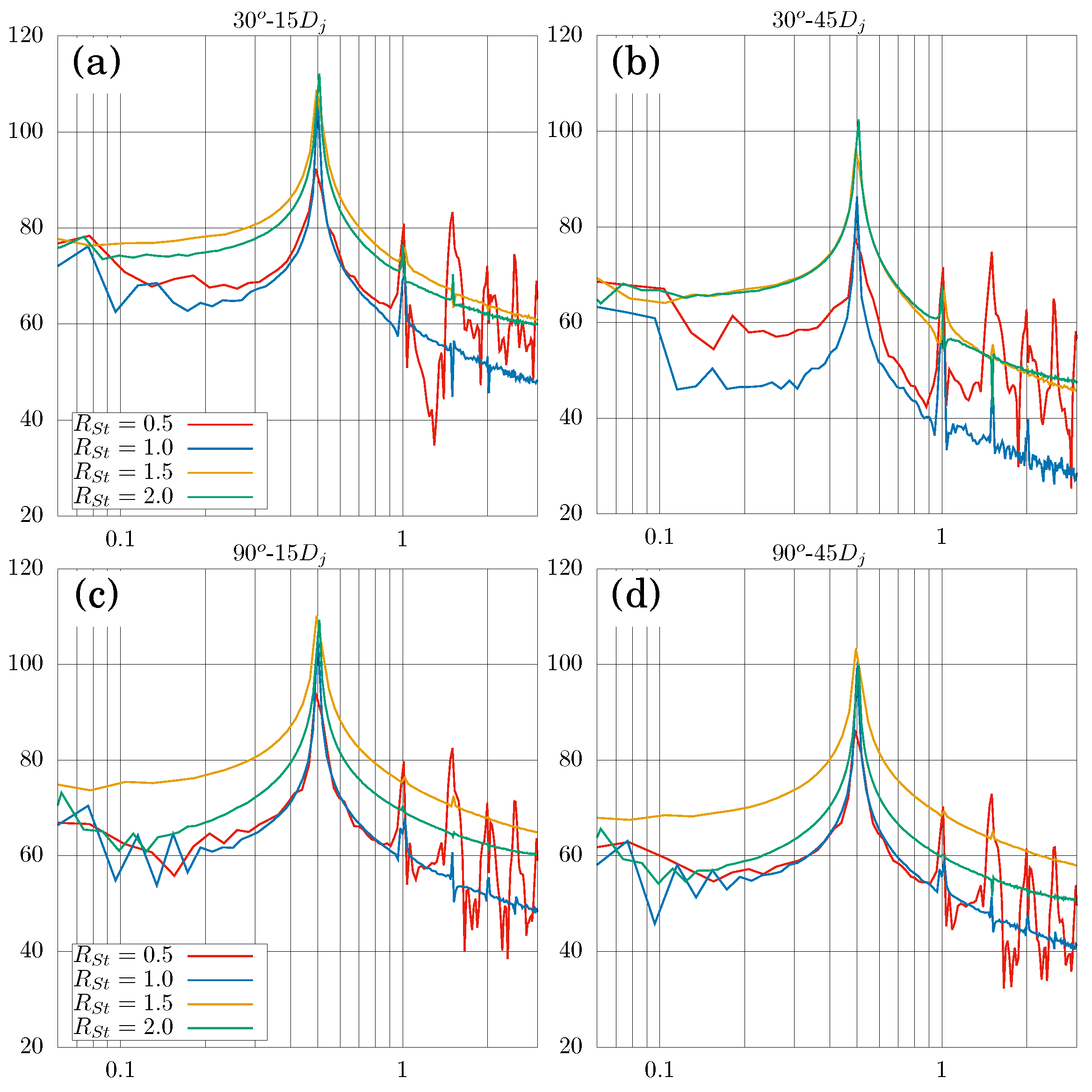
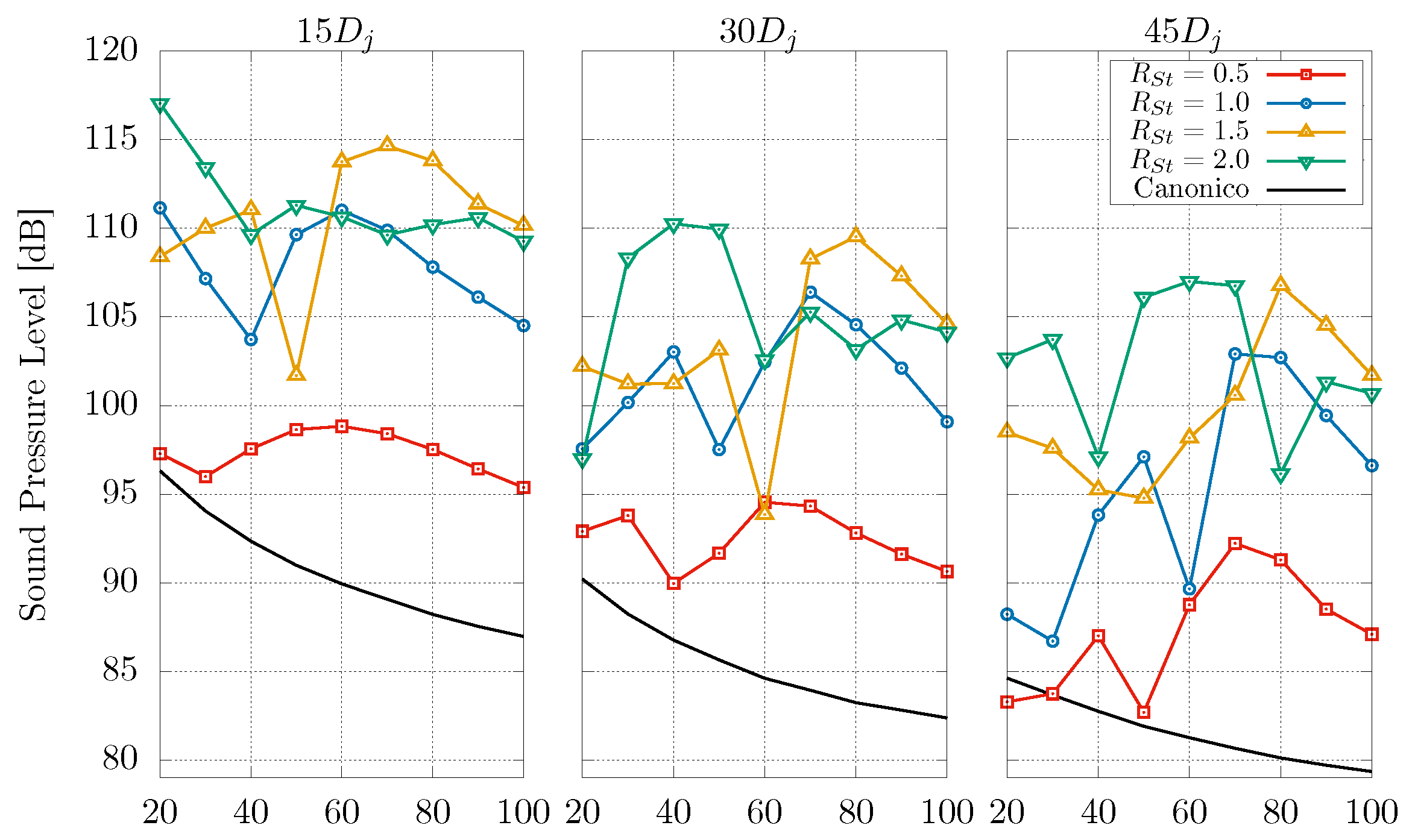
3.3. Acoustic Response
4. Conclusions
Supplementary Materials
Author Contributions
Funding
Institutional Review Board Statement
Informed Consent Statement
Data Availability Statement
Conflicts of Interest
References
- Kramer, C.; Gerhardt, H.; Knoch, M. Applications of jet flows in industrial flow circuits. J. Wind Eng. Ind. Aerodyn. 1984, 16, 173–188. [Google Scholar] [CrossRef]
- Gerges, S.; Sehrndt, G.; Parthey, W. 5 Noise Sources. In Occupational Exposure to Noise; World Health Organization: Geneva, Switzerland, 2001. [Google Scholar]
- Sheen, S.C.; Hsiao, Y.H. On using multiple-jet nozzles to suppress industrial jet noise. J. Occup. Environ. Hyg. 2007, 4, 669–677. [Google Scholar] [CrossRef] [PubMed]
- Sadeghian, M.; Bandpy, M. Technologies for Aircraft Noise Reduction: Review Paper. J. Aeronaut. Aerosp. Eng. 2020, 9, 218. [Google Scholar]
- WHO. Environmental Noise Guidelines for the European Region; World Health Organization: Geneva, Switzerland, 2018.
- Ahuja, K.; Bushell, K. An experimental study of subsonic jet noise and comparison with theory. J. Sound Vib. 1973, 30, 317–IN1. [Google Scholar] [CrossRef]
- Tam, C.K.; Tanna, H. Shock associated noise of supersonic jets from convergent-divergent nozzles. J. Sound Vib. 1982, 81, 337–358. [Google Scholar] [CrossRef]
- Viswanathan, K. Investigation of noise source mechanisms in subsonic jets. AIAA J. 2008, 46, 2020–2032. [Google Scholar] [CrossRef]
- Howe, M.S.; Howe, M.S. Acoustics of Fluid-Structure Interactions; Cambridge University Press: Cambridge, UK, 1998. [Google Scholar]
- Tam, C.; Golebiowski, M.; Seiner, J. On the two components of turbulent mixing noise from supersonic jets. In Proceedings of the Aeroacoustics Conference, State College, PA, USA, 6–8 May 1996; p. 1716. [Google Scholar]
- Camussi, R. Noise Sources in Turbulent Shear Flows: Fundamentals and Applications; Springer Science & Business Media: Berlin/Heidelberg, Germany, 2013; Volume 545. [Google Scholar]
- Henderson, B. Fifty years of fluidic injection for jet noise reduction. Int. J. Aeroacoust. 2010, 9, 91–122. [Google Scholar] [CrossRef]
- Rajput, P.; Kumar, S. Use of downstream fluid injection to reduce subsonic jet noise. Int. J. Aeroacoust. 2019, 18, 554–574. [Google Scholar] [CrossRef]
- Colonius, T.; Sinha, A.; Rodríguez, D.; Towne, A.; Liu, J.; Brès, G.; Appelö, D.; Hagstrom, T. Simulation and modeling of turbulent jet noise. In Direct and Large-Eddy Simulation IX; Springer: Berlin/Heidelberg, Germany, 2015; pp. 305–310. [Google Scholar]
- Callender, B.; Gutmark, E.; Martens, S. A comprehensive study of fluidic injection technology for jet noise reduction. In Proceedings of the 13th AIAA/CEAS Aeroacoustics Conference (28th AIAA Aeroacoustics Conference), Rome, Italy, 21–23 May 2007; p. 3608. [Google Scholar]
- Dhamankar, N.S.; Blaisdell, G.A.; Lyrintzis, A.S. Analysis of turbulent jet flow and associated noise with round and chevron nozzles using large eddy simulation. In Proceedings of the 22nd AIAA/CEAS Aeroacoustics Conference, Lyon, France, 30 May–1 June 2016; p. 3045. [Google Scholar]
- Stich, G.D.; Housman, J.A.; Ghate, A.S.; Kiris, C.C. Jet Noise Prediction with Large-Eddy Simulation for Chevron Nozzle Flows. In Proceedings of the AIAA Scitech 2021 Forum, Virtual Event, 11–15 January 2021; p. 1185. [Google Scholar]
- Powell, A. The influence of the exit velocity profile on the noise of a jet. Aeronaut. Q. 1954, 4, 341–360. [Google Scholar] [CrossRef]
- Kurbjun, M.C. Limited Investigation of Noise Suppression by Injection of Water into Exaust of Afterburning Jet Engine; National Advisory Committee for Aeronautics: Edwards, CA, USA, 1958; Volume 40. [Google Scholar]
- Michael, L.G. Jet Noise Suppression Means. U.S. Patent 2,990,905, 4 July 1961. [Google Scholar]
- Caeti, R.B.; Kalkhoran, I.M. Jet noise reduction via fluidic injection. AIAA J. 2014, 52, 26–32. [Google Scholar] [CrossRef]
- Prasad, C.; Morris, P.J. A study of noise reduction mechanisms of jets with fluid inserts. J. Sound Vib. 2020, 476, 115331. [Google Scholar] [CrossRef]
- Wang, J.; Feng, L. Synthetic Jet. In Flow Control Techniques and Applications; Cambridge Aerospace Series; Cambridge University Press: Cambridge, UK, 2018; pp. 168–205. [Google Scholar] [CrossRef]
- Chedevergne, F.; Léon, O.; Bodoc, V.; Caruana, D. Experimental and numerical response of a high-Reynolds-number M = 0.6 jet to a Plasma Synthetic Jet actuator. Int. J. Heat Fluid Flow 2015, 56, 1–15. [Google Scholar] [CrossRef]
- Zong, H.; Chiatto, M.; Kotsonis, M.; De Luca, L. Plasma synthetic jet actuators for active flow control. Proc. Actuators 2018, 7, 77. [Google Scholar] [CrossRef] [Green Version]
- Glezer, A. Some aspects of aerodynamic flow control using synthetic-jet actuation. Philos. Trans. R. Soc. A Math. Phys. Eng. Sci. 2011, 369, 1476–1494. [Google Scholar] [CrossRef] [PubMed]
- Tamburello, D.A.; Amitay, M. Active control of a free jet using a synthetic jet. Int. J. Heat Fluid Flow 2008, 29, 967–984. [Google Scholar] [CrossRef]
- Léon, O.; Caruana, D.; Castelain, T. Increase and decrease of the noise radiated by high-Reynolds-number subsonic jets through plasma synthetic jet actuation. In Proceedings of the International Conference on Acoustic Climate Inside and Outside Buildings, Vilnius, Lithuania, 23–26 September 2014; pp. 23–26. [Google Scholar]
- Arafa, N.; Sullivan, P.E.; Ekmekci, A. Jet Velocity and Acoustic Excitation Characteristics of a Synthetic Jet Actuator. Fluids 2022, 7, 387. [Google Scholar] [CrossRef]
- Lighthill, M.J. On sound generated aerodynamically I. General theory. Proc. R. Soc. Lond. Ser. A Math. Phys. Sci. 1952, 211, 564–587. [Google Scholar]
- Ffowcs Williams, J.E.; Hawkings, D.L. Sound generation by turbulence and surfaces in arbitrary motion. Philos. Trans. R. Soc. Lond. Ser. A Math. Phys. Sci. 1969, 264, 321–342. [Google Scholar]
- Brès, G.; Jordan, P.; Jaunet, V.; Le Rallic, M.; Cavalieri, A.; Towne, A.; Lele, S.; Colonius, T.; Schmidt, O. Importance of the nozzle-exit boundary-layer state in subsonic turbulent jets. J. Fluid Mech. 2018, 851, 83–124. [Google Scholar] [CrossRef] [Green Version]
- Panchapakesan, N.R.; Lumley, J.L. Turbulence measurements in axisymmetric jets of air and helium. Part 1. Air jet. J. Fluid Mech. 1993, 246, 197–223. [Google Scholar] [CrossRef]
- Moura, R.C.; Sherwin, S.J.; Peiró, J. Linear dispersion–diffusion analysis and its application to under-resolved turbulence simulations using discontinuous Galerkin spectral/hp methods. J. Comput. Phys. 2015, 298, 695–710. [Google Scholar] [CrossRef] [Green Version]
- Manneville, P.; Rolland, J. On modelling transitional turbulent flows using under-resolved direct numerical simulations: The case of plane Couette flow. Theor. Comput. Fluid Dyn. 2011, 25, 407–420. [Google Scholar] [CrossRef] [Green Version]
- Komen, E.; Shams, A.; Camilo, L.; Koren, B. Quasi-DNS capabilities of OpenFOAM for different mesh types. Comput. Fluids 2014, 96, 87–104. [Google Scholar] [CrossRef]
- Bosshard, C.; Deville, M.O.; Dehbi, A.; Leriche, E. UDNS or LES, that is the question. Open J. Fluid Dyn. 2015, 5, 339. [Google Scholar] [CrossRef] [Green Version]
- Ramirez-Pastran, J.; Duque-Daza, C. On the prediction capabilities of two SGS models for large-eddy simulations of turbulent incompressible wall-bounded flows in OpenFOAM. Cogent Eng. 2019, 6, 1679067. [Google Scholar] [CrossRef]
- LarKermani, E.; Roohi, E.; Porté-Agel, F. Evaluating the modulated gradient model in large eddy simulation of channel flow with OpenFOAM. J. Turbul. 2018, 19, 600–620. [Google Scholar] [CrossRef]
- Epikhin, A.; Evdokimov, I.; Kraposhin, M.; Kalugin, M.; Strijhak, S. Development of a Dynamic Library for Computational Aeroacoustics Applications Using the OpenFOAM Open Source Package. Procedia Comput. Sci. 2015, 66, 150–157. [Google Scholar] [CrossRef] [Green Version]
- Curle, N. The influence of solid boundaries upon aerodynamic sound. Proc. R. Soc. Lond. Ser. A. Math. Phys. Sci. 1955, 231, 505–514. [Google Scholar]
- Geuzaine, C.; Remacle, J.F. Gmsh: A 3-D Finite Element Mesh Generator with built-in Pre- and Post-Processing Facilities. Int. J. Numer. Methods Eng. 2009, 79, 1309–1331. [Google Scholar] [CrossRef]
- Bogey, C.; Marsden, O.; Bailly, C. Influence of initial turbulence level on the flow and sound fields of a subsonic jet at a diameter-based Reynolds number of 10 (5). J. Fluid Mech. 2012, 701, 352–385. [Google Scholar] [CrossRef] [Green Version]
- Mendez, S.; Shoeybi, M.; Lele, S.; Moin, P. On the use of the Ffowcs Williams-Hawkings equation to predict far-field jet noise from large-eddy simulations. Int. J. Aeroacoust. 2013, 12, 1–20. [Google Scholar] [CrossRef]
- Shin, D.H.; Aparece-Scutariu, V.; Richardson, E. High Fidelity Simulation of Turbulent Jet and Identification of Acoustic Sources. Civ. Aircr. Des. Res. 2017, 3, 1–9. [Google Scholar] [CrossRef]
- Todde, V.; Spazzini, P.G.; Sandberg, M. Experimental analysis of low-Reynolds number free jets. Exp. Fluids 2009, 47, 279–294. [Google Scholar] [CrossRef]
- Sautet, J.; Stepowski, D. Dynamic behaviour of variable-density, turbulent jets in their near development fields. Phys. Fluids 1995, 7, 2796–2806. [Google Scholar] [CrossRef]
- Bonelli, F.; Viggiano, A.; Magi, V. High-speed turbulent gas jets: An LES investigation of Mach and Reynolds number effects on the velocity decay and spreading rate. Flow Turbul. Combust. 2021, 107, 519–550. [Google Scholar] [CrossRef]
- Hussein, H.J.; Capp, S.P.; George, W.K. Velocity measurements in a high-Reynolds-number, momentum-conserving, axisymmetric, turbulent jet. J. Fluid Mech. 1994, 258, 31–75. [Google Scholar] [CrossRef] [Green Version]
- Viswanathan, K. Aeroacoustics of hot jets. In Proceedings of the 8th AIAA/CEAS Aeroacoustics Conference & Exhibit, Breckenridge, CO, USA, 17–19 June 2004; p. 2481. [Google Scholar]
- Jordan, E.L.P.; Delville, J.; Bonnet, J.P. Source-mechanism identification by nearfield-farfield pressure correlations in subsonic jets. Int. J. Aeroacoust. 2008, 7, 41–68. [Google Scholar] [CrossRef]


| Parameter | Value | Units (SI) |
|---|---|---|
| Diameter () | m | |
| Velocity () | 27 | m/s |
| Viscosity () | m/s | |
| Temperature (T) | K | |
| Mach number () | ≈0.1 | - |
| Reynolds number () | ≈11 | - |
| (Hz) | |
|---|---|
| 0.5 | 3803.88 |
| 1.0 | 7607.77 |
| 1.5 | 11,411.66 |
| 2.0 | 15,215.55 |
Disclaimer/Publisher’s Note: The statements, opinions and data contained in all publications are solely those of the individual author(s) and contributor(s) and not of MDPI and/or the editor(s). MDPI and/or the editor(s) disclaim responsibility for any injury to people or property resulting from any ideas, methods, instructions or products referred to in the content. |
© 2023 by the authors. Licensee MDPI, Basel, Switzerland. This article is an open access article distributed under the terms and conditions of the Creative Commons Attribution (CC BY) license (https://creativecommons.org/licenses/by/4.0/).
Share and Cite
Murillo-Rincón, J.; Duque-Daza, C. Evaluation of Synthetic Jet Flow Control Technique for Modulating Turbulent Jet Noise. Fluids 2023, 8, 110. https://doi.org/10.3390/fluids8040110
Murillo-Rincón J, Duque-Daza C. Evaluation of Synthetic Jet Flow Control Technique for Modulating Turbulent Jet Noise. Fluids. 2023; 8(4):110. https://doi.org/10.3390/fluids8040110
Chicago/Turabian StyleMurillo-Rincón, Jairo, and Carlos Duque-Daza. 2023. "Evaluation of Synthetic Jet Flow Control Technique for Modulating Turbulent Jet Noise" Fluids 8, no. 4: 110. https://doi.org/10.3390/fluids8040110