Numerical Analysis of Linear Traveling Wave in Rotating Rayleigh–Bénard Convection with an Adiabatic Sidewall

Abstract

In rotating Rayleigh–Bénard problems, convection with traveling waves may occur near the sidewalls. The Rayleigh number, Taylor number and Prandtl number are involved in this phenomenon, and the convection mode is determined depending on their values. We focused on the onset of this convection with traveling waves under the assumption that centrifugal force is neglected. By conducting two-dimensional linear stability analyses assuming periodicity of the flow and temperature fields along the sidewall direction, we investigated the effect of the Taylor number and the Prandtl number on the critical Rayleigh number and also attempted to understand the phenomenon qualitatively through three-dimensional visualizations. It was exhibited that as the Taylor number increases, the wave number, the Rayleigh number and the phase speed are found to increase. On the other hand, as the Prandtl number decreases, the wavenumber and the Rayleigh number decrease, but the phase velocity increases. The present analyses suggest that convection modes localized near the sidewalls are unlikely to emerge for low Prandtl number cases, which are comparable to those of liquid metals.

1. Introduction

Convection caused by bottom heating and top cooling of a horizontal fluid layer is called Rayleigh–Bénard convection. It is so named today after Bénard [1], who observed the convection pattern from an academic point of view, and Rayleigh [2], who first proposed a theory to explain it. In the system governed by the Navier–Stokes equations and the heat advection–diffusion equation, a linear stability analysis can be performed under the assumptions of the incompressible flow, the Boussinesq approximation and neglecting nonlinear terms. Initially, in this type of study, the thickness of the horizontal fluid layer was assumed to be sufficiently small compared to the horizontal scales, and the influence of sidewalls was not taken into consideration. In such cases, the factors involved in the onset of convection include the Rayleigh number as well as the upper and lower boundary conditions where the fluid layer is in contact.

Chandrasekar [3] employed linear stability analysis to investigate not only the instability of the Rayleigh–Bénard convection, but also the effects of Coriolis force and/or electromagnetic force due to the application of an external magnetic field. It is known that the critical state for the onset of convection in the so-called ordinary Rayleigh–Bénard problem without the influence of the rotational field is determined only by the Rayleigh number. The convection is a standing wave without accompanying phase velocity. However, in the Rayleigh–Bénard problem under the Coriolis force, according to Chandrasekar [3], oscillatory convection called overstability takes place. In the studies of Chandrasekar [3,4,5], one-dimensional linear analysis was performed neglecting centrifugal forces and assuming horizontal periodicity of the flow and temperature fields. Therefore, the influence of sidewalls was not taken into account. Kloosterziel and Carnevale [6] focused on the Chandrasekar’s work with the case of stress-free upper and lower boundaries, and they found simple expressions for the marginal stability boundary using the curve of the Taylor number as a function of the Rayleigh number and Prandtl number.

Subsequent experimental, theoretical and numerical studies have reported that convection in rotating Rayleigh–Bénard convection at a certain high Taylor number regime exhibits a wave-like behavior such that the flow is dominant near the sidewall of enclosure. Zhong et al. [7] made an optical shadowgraph flow visualization and heat transport measurements of the Rayleigh–Bénard convection of water confined in a cylindrical enclosure with an aspect ratio of 1. They showed that the onset of convection occurs at a much smaller Rayleigh number than that predicted by linear stability analysis for a laterally infinite system, and this is qualitatively consistent with finite-aspect-ratio linear-stability calculations of Buell and Catton [8]. Ning and Ecke [9] studied the initial bifurcations in rotating Rayleigh–Bénard convection for a cylindrical cell with an aspect ratio of 2.5. They used simultaneous optical-shadowgraph, heat-transport and local-temperature measurements to determine the stability and characteristics of the azimuthally periodic wall convection state. Their results for critical Rayleigh numbers, precession frequencies and critical mode numbers agreed well with theoretical results. Liu and Ecke [10] made similar experimental measurements for a sidewall traveling wave in rotating Rayleigh–Bénard convection of water (Pr = 6.3) in a cylinder (aspect ratio 5).

Kuo and Cross [11] showed that the wall-localized convection states observed in Rayleigh–Bénard convection in rotating cylindrical cells can be explained in terms of a geometry-independent traveling-wave wall state. They calculated the onset Rayleigh number, frequency and wave number of such a state, as well as its amplitude equation. Herrmann and Busse [12] derived asymptotic expressions for the onset of convection in a horizontal fluid layer of finite extent heated from below and rotating about a vertical axis in the limit of large rotation rates in the case of stress-free upper and lower boundaries. They found that critical Rayleigh number Ra_c grows in proportion to Ta^1/2, where Ta is the Taylor number, when the sidewall is insulating, whereas it grows in proportion to Ta^2/3 when the sidewall is infinitely conducting.

Goldstein et al. [13,14] studied the onset of convection in a uniformly rotating vertical cylinder heated from below. They showed that the spiral patterns typically precess counter to the rotation direction. In particular, two types of modes were distinguished: the fast modes with relatively high precession velocity whose amplitude peaks near the sidewall and the slow modes whose amplitude peaks near the center. Results were presented for Prandtl numbers in the range of 6.7 $\le$ Pr $\le$ 7.0 in their paper of Part 1 [13], while specific predictions were made for the Prandtl numbers at 0.025, 0.49 and 0.78 in that of Part 2 [14]. Bajaj et al. [15] studied rotating Rayleigh–Bénard convection for a small Prandtl number using a H₂-Xe gas mixture whose Prandtl number was about 0.18.

Plaut [16] analyzed weakly nonlinear dynamics of the traveling-wave sidewall modes appearing in rotating Rayleigh–Bénard convection using the Ginzburg–Landau envelope equation. Scheel [17] derived the amplitude equation for rotating Rayleigh–Bénard convection. The results of amplitude equation for a specific set of parameters were compared with numerical results from simulations of the full equations. Tagare et al. [18] investigated linear and weakly nonlinear properties of Rayleigh–Bénard convection in rotating fluids. They derived a nonlinear one-dimensional Landau–Ginzburg equation with real coefficients near the onset of stationary convection at the supercritical pitchfork bifurcation. Husain et al. [19] carried out three-dimensional numerical investigation of rotating Rayleigh–Bénard convection in a large-aspect-ratio (8:8:1) rectangular enclosure. The simulations were carried out for liquid metal flows with Pr = 0.01 and Ra = 10⁷, while the rotational Rayleigh number and the Taylor number were varied through non-dimensional rotation rate.

Research reports on rotating Rayleigh–Bénard convection can be found even in recent years. Yu et al. [20] determined convection patterns that occur at and slightly above the onset of Rayleigh–Bénard convection in cylindrical containers as a function of aspect ratio, using simulations and linear stability analyses. Their study focused primarily on the aspect ratios 6 to 20 with conducting or insulating sidewalls and Prandtl numbers Pr = 0.7 and 28.9. Favier et al. [21] explored the possibility of subcritical behavior in the geostrophic turbulence regime of rapidly rotating thermally driven convection. Favier and Knobloch [22] showed that wall modes in Rayleigh–Bénard convection in a rapidly rotating cylinder persist even very far from their linear onset.

Other recent studies related to rotating Rayleigh–Bénard convection include research on dynamics and statistics of reorientations of large-scale circulation (LSC) in turbulence [23], horizontal translational motion of columnar vortices formed in rotating Rayleigh–Bénard convection [24], spatially resolved measurements of the columnar vortex structures [25], inverse cascade and flow speed scaling behavior [26], force balance [27], understanding the dynamics of large-scale vortices (LSVs) in gas giants [28] and the context of geophysics and astrophysics [29,30].

In summary, in the rotating Rayleigh–Bénard problem, the convection mode is variously influenced by the upper and the lower boundaries, the thermal condition of the sidewalls, the speed of enclosure rotation (the Taylor number), the Prandtl number and the aspect ratio of the enclosure. In the present study, from a fundamental viewpoint, the works of Kuo and Cross [11] and Plaut [16] are extended to determine the onset of wave-type convection observed along the vertical sidewall of an enclosure. Particularly, we focus on obtaining critical Rayleigh numbers, horizontal wavenumbers, phase velocities and flow structures using a developed numerical method for linear stability analysis. Furthermore, the influence of heating condition at the bottom wall is further discussed.

2. Mathematical Formulations

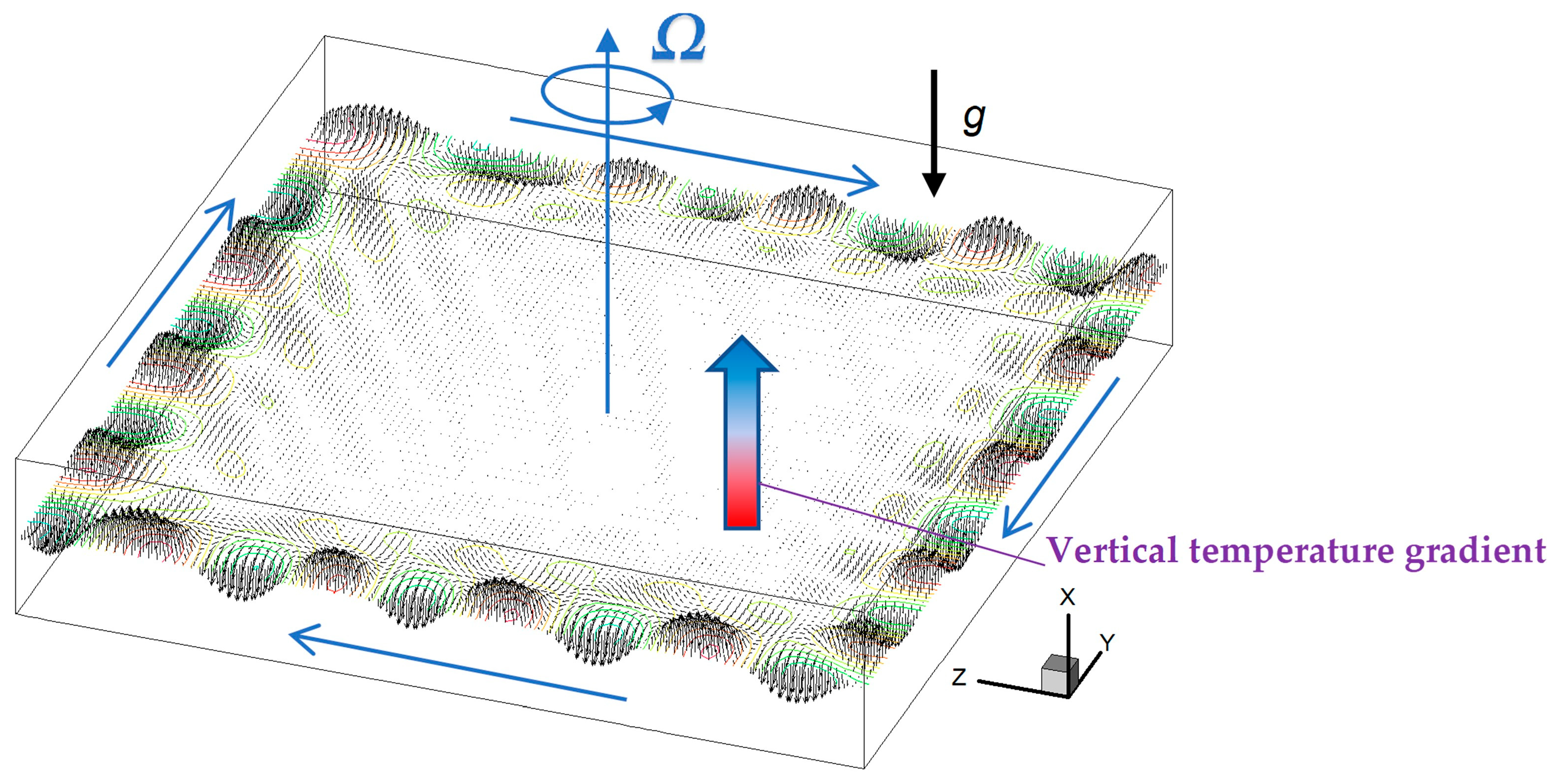
2.1. Schematic Model for Rotating Rayleigh–Bénard Convection

Rayleigh–Bénard convection in a rectangular enclosure rotating at a constant angular velocity, whose vector is parallel to the direction of gravity, is considered as illustrated in Figure 1. The height of the fluid layer is taken as the representative length. In the rotating frame of reference, it is known that the Coriolis force and the centrifugal force appear in the equation of motion, but the mass conservation equation and the energy equation are not modified. It is assumed that the sidewalls of the enclosure are adiabatic, the bottom wall is heated at a constant temperature or heat flux and the top wall is cooled at a constant temperature.

2.2. Governing Equations

When we consider a fluid flow with a constant density, such as a single-phase isothermal field, the centrifugal force is a conservative force, just like gravity. In this case, the centrifugal force does not affect the flow, but merely changes the pressure field. However, the centrifugal buoyancy force may act in the direction perpendicular to the rotation axis for the flow treated in this study where the fluid density depends on the temperature. In Rayleigh–Bénard convection without rotation, a perfect heat conduction state is realized when the Rayleigh number is less than its critical value, whereas in Rayleigh–Bénard convection subjected to rotating condition, a weak convection occurs due to the effect of centrifugal buoyancy. Hence, the state of pure heat conduction may not be realized. The ratio of centrifugal force to gravity is expressed using the Froude number. If this value is small, the centrifugal force is negligible relative to gravity. In fact, in Chandrasekhar’s analysis of rotating Rayleigh–Bénard convection, the pure heat conduction state ignoring the centrifugal force effect is regarded as the basic state for the linear stability analysis. Therefore, in this study, we decided to perform the linear stability analysis ignoring the centrifugal force effect.

The governing equations are the incompressible continuity equation, the momentum equation with the Boussinesq approximation and the energy equation. Each is shown below. The x-axis of the Cartesian coordinate system is taken in vertical, and the y- and z-axes are taken in horizontal:

Continuity of mass:

$$\nabla \cdot \mathit{u}=0;$$

(1)

Momentum equations:

$$\frac{\partial \mathit{u}}{\partial t}+\mathit{u}\cdot \nabla \mathit{u}=-\frac{1}{{\rho }_0}\nabla p+\nu {\nabla }^2\mathit{u}+g\beta \left(T-T_0\right){\mathit{e}}_x+2\Omega \mathit{u}\times {\mathit{e}}_x;$$

(2)

Energy equation:

$$\frac{\partial T}{\partial t}+\mathit{u}\cdot \nabla T=\alpha {\nabla }^{2}T;$$

(3)

Boundary conditions:

$$\left\{\begin{array}{l}x=h:\hspace{1em}u=v=w=0,\hspace{1em}T=T_c\\ x=0:\hspace{1em}u=v=w=0,\hspace{1em}T=T_h\hspace{1em}or\hspace{1em}q=-\lambda \frac{\partial T}{\partial x}=const.\end{array}\right..$$

(4)

3. Linear Stability Analysis (LSA)

3.1. Basic State

The basic state is assumed to be in heat conduction with no convection. The temperature and pressure gradients are given by the following equations, respectively. In this study, the temperature difference is defined as $\Delta T=T_h-T_c$ (during isothermal heating) or $\Delta T=qh/\lambda$ (during uniform flux heating):

$$\overline{u}=\overline{v}=\overline{w}=0,\hspace{1em}\overline{T}\left(x\right)=T_h-\Delta T\frac{x}{h},\hspace{1em}\frac{\partial \overline{p}}{\partial y}=\frac{\partial \overline{p}}{\partial z}=0,\hspace{1em}\frac{\partial \overline{p}}{\partial x}={\rho }_{0}g\beta \Delta T\left(\frac{1}{2}-\frac{x}{h}\right).$$

(5)

3.2. Disturbance Equations

3.2.1. One-Dimensional LSA

In one-dimensional analysis, the effects of sidewalls cannot be taken into account. In the Cartesian coordinate system, the linearized perturbation equations are expressed as follows:

$$\nabla \cdot \mathit{u}\prime =0,$$

(6)

$$\frac{\partial \mathit{u}\prime }{\partial t}=-\frac{1}{{\rho }_0}\nabla p\prime +\nu {\nabla }^2\mathit{u}\prime +g\beta T\prime {\mathit{e}}_x+2\Omega \left(w\prime {\mathit{e}}_y-v\prime {\mathit{e}}_z\right),$$

(7)

$$\frac{\partial T\prime }{\partial t}=\frac{\Delta T}{h}u\prime +\alpha {\nabla }^{2}T\prime .$$

(8)

The boundary conditions for the perturbed quantities are as follows:

$$\left\{\begin{array}{l}x=h:\hspace{1em}u\prime =v\prime =w\prime =0,\hspace{1em}T\prime =0\\ x=0:\hspace{1em}u\prime =v\prime =w\prime =0,\hspace{1em}T\prime =0\hspace{1em}or\hspace{1em}\frac{\partial T\prime }{\partial x}=0\end{array}\right..$$

(9)

Furthermore, each variable is assumed to be using a complex amplitude function, as follows:

$$\varphi \prime \left(x,y,z,t\right)=\tilde{\varphi }\left(x\right)\exp \left\{i\left(a_{y}y+a_{z}z\right)+st\right\}+\mathrm{c}.\mathrm{c}.,$$

(10)

where a_y and a_z represent the wavenumbers in the y- and z-directions, respectively. Furthermore, i represents the imaginary unit, and s is a complex number whose real part indicates the linear growth rate and whose imaginary part is the angular frequency. Substituting Equation (10) into Equations (6)–(9), and making it dimensionless, the simultaneous ordinary equations for the amplitude function can be summarized as follows:

$$D\tilde{U}+i\left(k_Y\tilde{V}+k_Z\tilde{W}\right)=0,$$

(11)

$$S\tilde{U}=-D\tilde{P}+\left(D^2-k^2\right)\tilde{U}+Ra\tilde{\Theta },$$

(12)

$$S\tilde{V}=-i{k}_Y\tilde{P}+\left(D^2-k^2\right)\tilde{V}+T{a}^{1/2}\tilde{W},$$

(13)

$$S\tilde{W}=-i{k}_Z\tilde{P}+\left(D^2-k^2\right)\tilde{W}-T{a}^{1/2}\tilde{V},$$

(14)

$$PrS\tilde{\Theta }=\tilde{U}+\left(D^2-k^2\right)\tilde{\Theta },$$

(15)

where dimensionless variables and dimensionless numbers are defined as follows:

$$\begin{array}{l}\left(\tilde{U},\tilde{V},\tilde{W}\right)=\frac{\left(\tilde{u},\tilde{v},\tilde{w}\right)}{\alpha /h},\hspace{1em}\tilde{P}=\frac{\tilde{p}}{{\rho }_0\alpha \nu /h^2},\hspace{1em}\tilde{\Theta }=\frac{\tilde{T}}{\Delta T},\hspace{1em}\left(k_Y,k_Z\right)=\frac{\left(a_y,a_z\right)}{1/h},\hspace{1em}X=\frac{x}{h},\hspace{1em}D\equiv \frac{d}{dX},\hspace{1em}\\ k^2=k_Y{}^2+k_Z{}^2,\hspace{1em}S=\frac{s}{\nu /h^2},\hspace{1em}Ta={\left(\frac{2\Omega h^2}{\nu }\right)}^2,\hspace{1em}Ra=\frac{g\beta \Delta T{h}^3}{\alpha \nu },\hspace{1em}Pr=\frac{\nu }{\alpha }.\end{array}$$

(16)

3.2.2. Linear Stability Analysis of Traveling-Wave Sidewall Mode

In this subsection, we describe two-dimensional LSA, which is the main part of this paper. The x-axis is taken in the vertical direction in common with the one-dimensional analysis, but periodicity is assumed only in the z-axis direction. It is assumed that y = constant surface (sidewall) is thermally insulated, and the centrifugal force is neglected herein as well. The analysis area is an x-y cross-section. Therefore, it can be assumed that the basic state is a state of heat conduction with no convection. The temperature and pressure gradients are given by Equation (5). The linearized perturbation equations in the Cartesian coordinate system are the same as Equations (6)–(8). The boundary conditions for the perturbations are given by Equation (17) in addition to Equation (9). The aspect ratio (width to height) of the x-y cross-section of the enclosure was assumed to be 2, and a slip condition was applied to the boundary condition at the non-walled side (as can be seen from the actual analysis, y = 2h is the bulk region sufficiently away from the sidewall, where the magnitude of flow and temperature disturbances is nearly zero). The adiabatic conditions were imposed at y = 0 and 2h:

$$\left\{\begin{array}{l}y=2h:\hspace{1em}\frac{\partial u\prime }{\partial y}=\frac{\partial v\prime }{\partial y}=\frac{\partial w\prime }{\partial y}=\frac{\partial T\prime }{\partial y}=0\\ y=0:\hspace{1em}u\prime =v\prime =w\prime =\frac{\partial T\prime }{\partial y}=0\end{array}\right..$$

(17)

In the two-dimensional LSA, each variable is assumed to be as follows, using a complex amplitude function as shown in Equation (18):

$$\varphi \prime \left(x,y,z,t\right)=\tilde{\varphi }\left(x,y\right)\exp \left(i{a}_{z}z+st\right)+\mathrm{c}.\mathrm{c}..$$

(18)

The dimensionless system of the amplitude functions is summarized as follows:

$${\partial }_X\tilde{U}+{\partial }_Y\tilde{V}+ik\tilde{W}=0,$$

(19)

$$S\tilde{U}=-{\partial }_X\tilde{P}+\left({\partial }_X^2+{\partial }_Y^2-k^2\right)\tilde{U}+Ra\tilde{\Theta },$$

(20)

$$S\tilde{V}=-{\partial }_Y\tilde{P}+\left({\partial }_X^2+{\partial }_Y^2-k^2\right)\tilde{V}+T{a}^{1/2}\tilde{W},$$

(21)

$$S\tilde{W}=-ik\tilde{P}+\left({\partial }_X^2+{\partial }_Y^2-k^2\right)\tilde{W}-T{a}^{1/2}\tilde{V},$$

(22)

$$PrS\tilde{\Theta }=\tilde{U}+\left({\partial }_X^2+{\partial }_Y^2-k^2\right)\tilde{\Theta },$$

(23)

The dimensionless variables and dimensionless numbers for the two-dimensional LSA are defined similarly to Equation (16).

3.3. Numerical Methodology

According to the Chandrasekhar’s works [3,4,5], two kinds of convection mode in the rotating Rayleigh–Bénard problem are discussed. One is the stationary mode and the other is the oscillatory mode (overstability). According to references [3,4,5], the latter may occur when the Prandtl number is lower than the critical value of the Prandtl number (Pr_c = 0.6766). Here, we present a numerical calculation method for capturing these two modes, respectively.

3.3.1. One-Dimensional LSA with the Stationary Mode

When considering the neutral stability state in the stationary mode, the real and imaginary parts of S are both zero, and therefore this state is independent of the Prandtl number. In order to obtain this state, in this research, the simultaneous equations, in which virtual time-derivative terms are introduced into the equations of motion and energy, are numerically solved using the HSMAC (Highly Simplified Marker and Cell) method. It is necessary and sufficient to calculate the real part of the vertical velocity component, pressure, temperature and the imaginary part of the two horizontal velocity components. It can be regarded as an eigenvalue problem to find the neutral Rayleigh number when the wavenumber k is given. Therefore, by numerically solving the above simultaneous equations while modifying the Rayleigh number and continuing iterative calculations until the virtual time-derivative term becomes almost zero, the Rayleigh number as an eigenvalue and the corresponding eigenfunction (amplitude function) can be obtained. At the same time, the normalization of the eigenfunction was made by fixing the calculated value of an arbitrarily chosen amplitude function at an arbitrarily chosen grid point.

Next, we explain the iterative correction formula for obtaining the eigenvalues. From the equation of motion in the vertical direction:

$$f\left(Ra\right)=\frac{\partial {\tilde{U}}_R}{\partial \tau }=-D{\tilde{P}}_R+\left(D^2-k^2\right){\tilde{U}}_R+Ra{\tilde{\Theta }}_R=0.$$

(24)

Therefore, considering Newton’s method, we obtain the following iterative correction formula:

$$R{a}^{\left(m+1\right)}=R{a}^{\left(m\right)}-\frac{f\left(R{a}^{\left(m\right)}\right)}{\partial f/\partial Ra}=R{a}^{\left(m\right)}-C_1\frac{\Delta {\tilde{U}}_R{}^{\left(m\right)}}{{\tilde{\Theta }}_R{}^{\left(m\right)}},$$

(25)

where C₁ is a constant and it plays a role in adjusting the convergence speed. At an arbitrarily chosen grid point, the Rayleigh number can be converged by imposing this formula. The Rayleigh number obtained using the correction formula is the neutral Rayleigh number for the given wavenumber k.

3.3.2. Two-Dimensional LSA with the Oscillatory Mode

In this mode, we need to find both the angular frequency and linear growth rate. Therefore, unlike the stationary mode, it is necessary to calculate both the real and imaginary parts of each amplitude function. In order to acquire the oscillatory mode, we introduced a virtual time-derivative term to the equations of motion and the energy equation, and analyzed them via iterative calculation using the HSMAC method. In the analysis of oscillatory mode, the problem is reduced to finding the most unstable complex eigenvalue S and its corresponding eigenfunction for a given wavenumber k and a Rayleigh number Ra. For example, Equation (20) can be separated into the two real function equations as follows:

$$\begin{array}{l}f\left(S_R\right)=\frac{\partial {\tilde{U}}_R}{\partial \tau }=-\left(S_R{\tilde{U}}_R-S_I{\tilde{U}}_I\right)-{\partial }_X{\tilde{P}}_R+\left({\partial }_X^2+{\partial }_Y^2-k^2\right){\tilde{U}}_R+Ra{\tilde{\Theta }}_R\cong 0\\ f\left(S_I\right)=\frac{\partial {\tilde{U}}_I}{\partial \tau }=-\left(S_R{\tilde{U}}_I+S_I{\tilde{U}}_R\right)-{\partial }_X{\tilde{P}}_I+\left({\partial }_X^2+{\partial }_Y^2-k^2\right){\tilde{U}}_I+Ra{\tilde{\Theta }}_I\cong 0\end{array}.$$

(26)

The linear growth rate S_R was obtained by imposing the following equation during the iterative calculation:

$$S_R{}^{\left(m+1\right)}=S_R{}^{\left(m\right)}-C_2\frac{\Delta {\tilde{U}}_R{}^{\left(m\right)}}{{\tilde{U}}_R{}^{\left(m\right)}}.$$

(27)

Similarly, the angular frequency S_I was obtained via iterative calculation using the following equation:

$$S_I{}^{\left(m+1\right)}=S_I{}^{\left(m\right)}-C_3\frac{\Delta {\tilde{U}}_I{}^{\left(m\right)}}{{\tilde{U}}_R{}^{\left(m\right)}}.$$

(28)

Basically, the complex eigenvalue problem was circumvented in this way. In addition to this, the following iterative correction formula was imposed to obtain neutral Rayleigh number:

$$R{a}^{\left(m+1\right)}=R{a}^{\left(m\right)}-C_4{S}_R{}^{\left(m\right)}.$$

(29)

Using formula (29), the value of Ra changes little by little from the value of Ra once given, and, when it converges, the neutral Ra value is obtained. See references [31,32] for details of this technique.

4. Results

4.1. One-Dimensional LSA

4.1.1. Stationary Mode

Table 1. The critical Rayleigh numbers for various Taylor number (stationary mode).

Ta	k	Present Study		Chandrasekar [3] Ra
		Ra and Number of Grids
10	3.10	1.7128 × 103	400	1.7130 × 103
100	3.15	1.7564 × 103	400	1.7566 × 103
500	3.30	1.9403 × 103	400	1.9403 × 103
1000	3.50	2.1514 × 103	400	2.1517 × 103
2000	3.75	2.5301 × 103	400	2.5305 × 103
5000	4.25	3.4686 × 103	400	3.4686 × 103
10,000	4.80	4.7121 × 103	400	4.7131 × 103
30,000	5.80	8.3246 × 103	800	8.3264 × 103
105	7.20	1.6720 × 104	800	1.6721 × 104
106	10.80	7.1085 × 104	1600	7.1132 × 104
108	24.5	1.5252 × 106	3200	1.5313 × 106
1010	55.5	3.4498 × 107	6400	3.4574 × 107

shows the critical Rayleigh numbers for various Taylor numbers when the stationary mode is assumed. As long as the wavenumber k is the same, the critical value is uniquely determined no matter how the two horizontal wavenumbers are combined. In other words, the present calculation was performed with k_Z = k (k_Y = 0). A comparison with Chandrasekhar’s study [3] is shown. As the value of the Taylor number increases, the boundary layer formed near the heating or cooling wall becomes thinner, and it becomes difficult to maintain calculation accuracy with a coarse grid. Even for calculations with high Taylor numbers, we obtained a solution that does not depend on the number of grids by securing a sufficient number of grid points. At low Taylor numbers, the agreement with Chandrasekhar’s critical Rayleigh number is good. At high Taylor numbers, the Rayleigh number obtained by the present numerical calculation is slightly lower than that of Chandrasekhar. Regardless, the present numerical analysis code is judged to be valid.

Figure 2 shows the visualization for k = 4.8 and Ta = 10⁴. In order to perform two-dimensional visualization using the one-dimensional amplitude function results, the following conversion formula was used:

$$\varphi \left(X,Z\right)\equiv \Re \left(\varphi \prime \right)={\tilde{\varphi }}_R\left(X\right)\cos \left(kZ\right)-{\tilde{\varphi }}_I\left(X\right)\sin \left(kZ\right),$$

(30)

where φ is a general representation of (U, V, W, P, Θ). Since the vertical velocity U and the temperature Θ have the same phase, the temperature takes positive values where there is an upward velocity. The phases of V and W deviate from that of U. Therefore, the velocity vectors are rather deformed from a circular vortex. The pressure takes a maximum or a minimum value at the stagnation point of the velocity field.

4.1.2. Oscillatory Mode (Overstability)

In this subsection, we present the critical Rayleigh numbers for the overstability, which was reported by Chandrasekhar [3]. Depending on the value of the Prandtl number, various critical Rayleigh numbers would be obtained, but we limited ourselves to the case of Pr = 0.025 for the sake of comparison and validity.

Table 2. The dependency of the grids on the angular frequency and the Rayleigh number (Pr = 0.025).

Ta	k	SI			Ra
		Present Study		Chandrasekar	Present Study		Chandrasekar
		200 Grids	400 Grids		200 Grids	400 Grids
104	3.08	4.47036 × 101	4.47038 × 101	4.45 × 101	4.370328 × 103	4.370333 × 103	4.39 × 103
106	4.09	5.82579 × 102	5.82585 × 102	5.82 × 102	9.5102 × 103	9.5096 × 103	9.51 × 103
5 × 107	8.10	2.4258 × 103	2.4262 × 103	2.43 × 103	6.313 × 104	6.302 × 104	6.29 × 104
2 × 108	10.28	3.916 × 103	3.918 × 103	3.92 × 103	1.388 × 105	1.381 × 105	1.38 × 105
109	13.46	6.805 × 103	6.813 × 103	6.81 × 103	3.607 × 105	3.552 × 105	3.54 × 105
1010	19.70	1.489 × 104	1.494 × 104	1.50 × 104	1.520 × 106	1.436 × 106	1.42 × 106
1011	28.75	3.251 × 104	3.262 × 104	3.27 × 104	6.418 × 106	6.139 × 106	5.83 × 106

summarizes the overstability solutions obtained by the present numerical calculations. To show the convergence of the solution with the number of grids, both results of 200 and 400 grids are shown. As the Taylor number increases, boundary layer type flow and temperature fields are formed, revealing the insufficient number of grids. Compared to Chandrasekar’s solution, the angular frequency of the present results tends to be lower, while the Rayleigh number tends to be higher. However, when the number of grids is increased from 200 to 400, it tends to approach the solution obtained by Chandrasekhar, so the analysis method is judged to be valid.

Figure 3 shows the neutral stability curve of the Rayleigh number and the angular frequency obtained using 400 grids for Pr = 0.025 and Ta = 10⁶. This figure shows the dependence of the Rayleigh number and the angular frequency on the wavenumber, with the neutral stable state obtained at wavenumber steps of 0.1. It can be seen that it takes a local minimum at k = 4.1. As for the angular frequency, it looks like a linear change in this wavenumber range, but it is a slightly downward convex curve.

Figure 4 shows a visualization of the eigenfunctions when the instability sets in overstability. Since the calculation assumes periodicity in the Z-direction, the visualization for only one wavelength is shown herein as well. While maintaining this state, the wave moves from right to left (in the negative Z-direction) at a constant speed. It should be noted that that there exist solutions to this eigenvalue problem that have the same absolute value of the angular frequency and differ only in their sign. In that case, the critical Rayleigh number remains the same. The wave moves from left to right (positive Z-direction) because the eigenfunction distribution is left–right reversed.

Although the vertical velocity U and the temperature Θ are in the same phase, V, W and P are in different phases. At first glance, the appearance of the velocity vector is similar to that of the stationary convection, but it is slightly different in that the velocity is distorted in the boundary layer.

Let us compare the stationary convection in Table 1 and overstability in Table 2. It can be seen that, for the same Taylor number, the critical Rayleigh number for overstability is much lower than that for the stationary convection. Thus, for Pr = 0.025, the resulting flow is expected to emerge as overstability. In this one-dimensional analysis, the influence of the sidewall cannot be considered, so it is difficult to compare with experiments. Therefore, in the next section, the LSA analysis considering the sidewall is performed, and based on the results, the interpretation of the results of the one-dimensional analysis will be reconsidered.

4.2. Two-Dimensional LSA (Traveling-Wave Sidewall Mode)

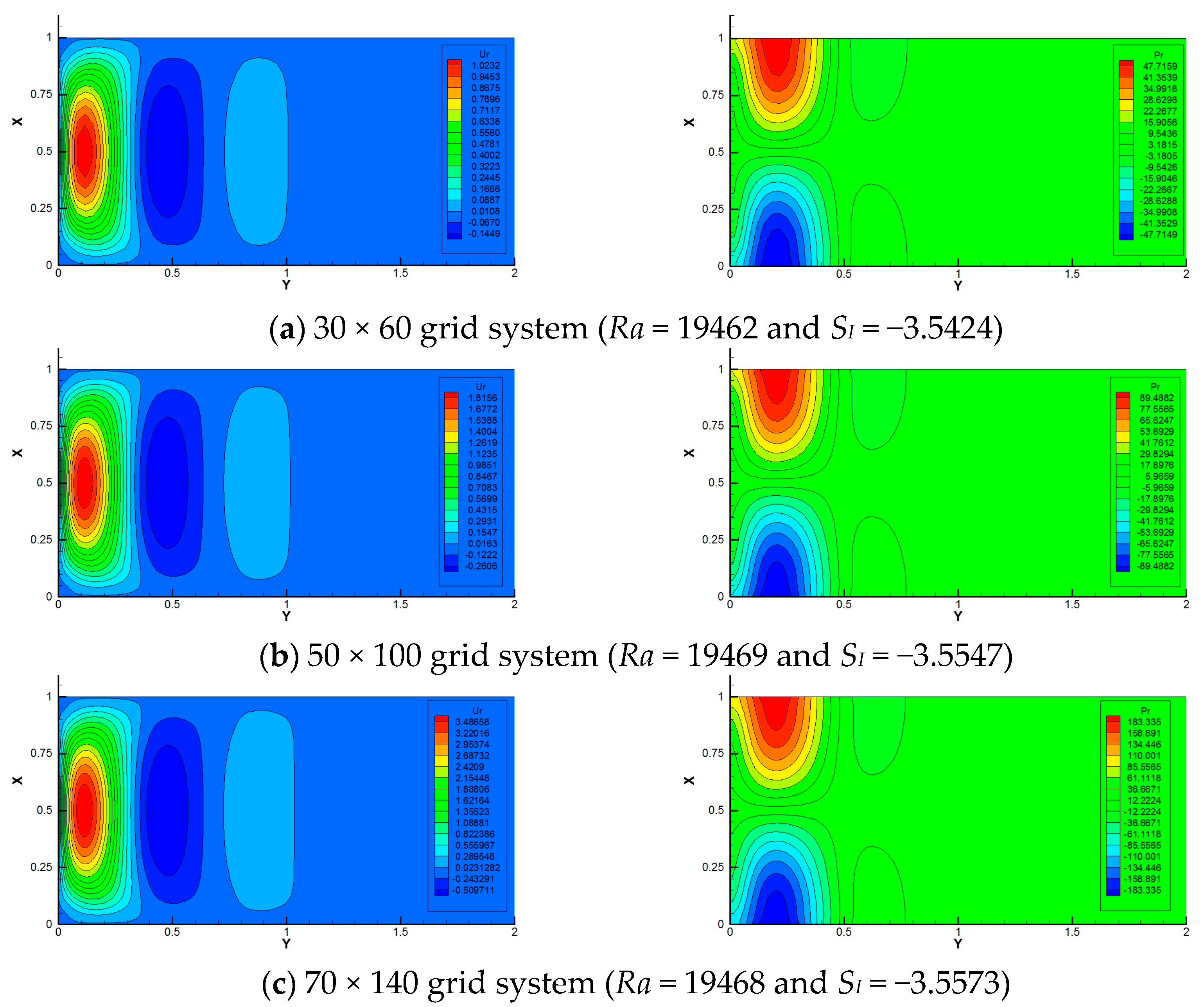
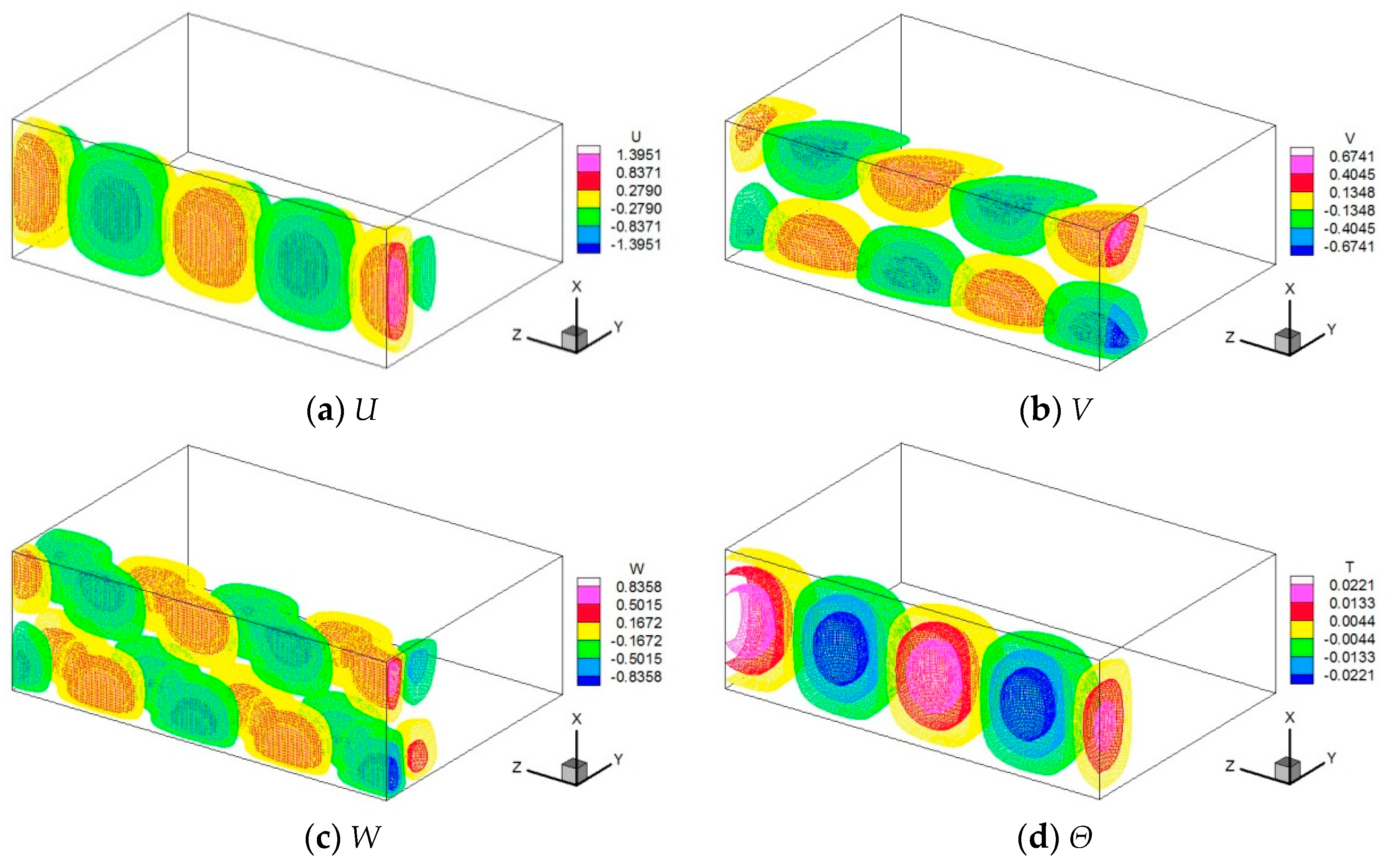
4.2.1. Verification of the Present Numerical Code

The number of grid points used in this two-dimensional analysis was set to 50 for the vertical and 100 for the horizontal directions due to computation time. Using this as a baseline, calculations were also performed for the 30 × 60 and the 70 × 140 grid systems to check the dependence on the number of grids employed.

First, a comparison with the previous study by Plaut [16] is performed to confirm the validity and accuracy of this analysis method. In that paper, comparisons are made with Liu and Ecke [10] as an experimental study and with Kuo and Cross [9] as a theoretical study. The dimensionless parameters are the Prandtl number Pr = 6.3 and the Coriolis number η = 548. In the present study, instead of using the Coriolis number, we used the Taylor number following Chandrasekar. Their dimensionless relation is given by Ta^1/2 = η. Therefore, η = 548 corresponds to Ta = 3 × 10⁵.

Figure 5 shows the neutral stability curve obtained by the present numerical analysis using the 50 × 100 grid system. The critical wavenumber, Rayleigh number and angular frequency were obtained to be approximately k_c = 4.225, Ra_c = 1.9649 × 10⁴ and S_I,c = −3.5547. To investigate the grid dependence on these critical values, numerical analyses were further performed using the 30 × 60 and the 70 × 140 grid systems. Figure 6 shows the eigenfunction distributions of vertical velocity and pressure in the X-Y cross-section. From the top to bottom, the 30 × 60, the 50 × 100 and the 70 × 140 grid systems are shown. It can be recognized that there is little qualitative difference in the eigenfunctions, and there are no significant differences in the neutral Rayleigh number and angular frequency. Therefore, the calculations using the 50 × 100 grid system are judged to be reasonable.

Table 3. Comparison of the important values between the previous results and the present result for Pr = 6.3 and Ta = 3 × 10⁵.

	Rac	kc	ωc
Expt. of Liu and Ecke [10]	20,850	4.65	−22.0
Theor. of Kuo and Cross [9]	19,500	4.00	−24.0
Theor. of Plaut [16]	19,660	4.22	−22.4
Present study	19,649	4.225	−22.39

summarizes the critical Rayleigh numbers, wavenumbers and angular frequencies obtained by the three previous studies and the present study. Since there is a difference in the dimensionless equations between these previous studies and the present study, the S_I value (−3.5547) was not used in its original form for the angular frequency, but was corrected by multiplying it by the value of the Prandtl number. As a result, the dimensionless angular frequency ω_c in this study was obtained as −22.39. Since Plaut’s results and our analysis results show good agreement, we judged that the 2D LSA analysis code is appropriate.

Figure 7 shows the isosurfaces of each eigenfunction at this critical state. The visualization range is two wavelengths in the z-axis direction. The flow field and temperature field are dominant near the sidewall at Y = 0, while no disturbance is observed in the region far from the sidewall. Since this disturbance has a negative angular frequency, it proceeds in the positive direction along the z-axis. The vertical velocity component and temperature are even functions with respect to the center of X, while the horizontal velocity components are odd functions, similar to the one-dimensional analysis of overstability. The vertical velocity U and the temperature Θ were in the same phase in the case of overstability where sidewalls cannot be considered, but they differ in that they have a phase difference in the traveling wave.

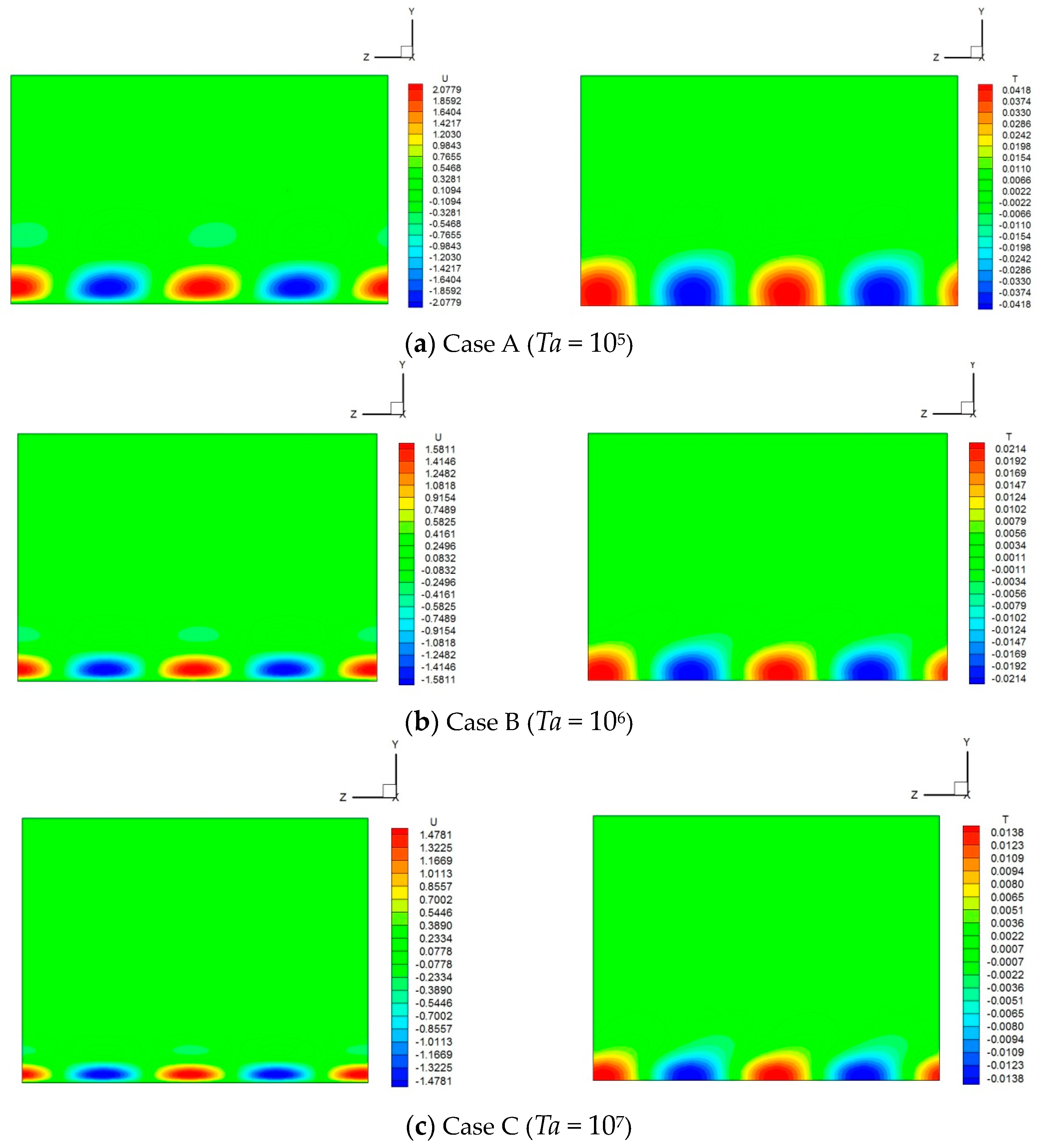
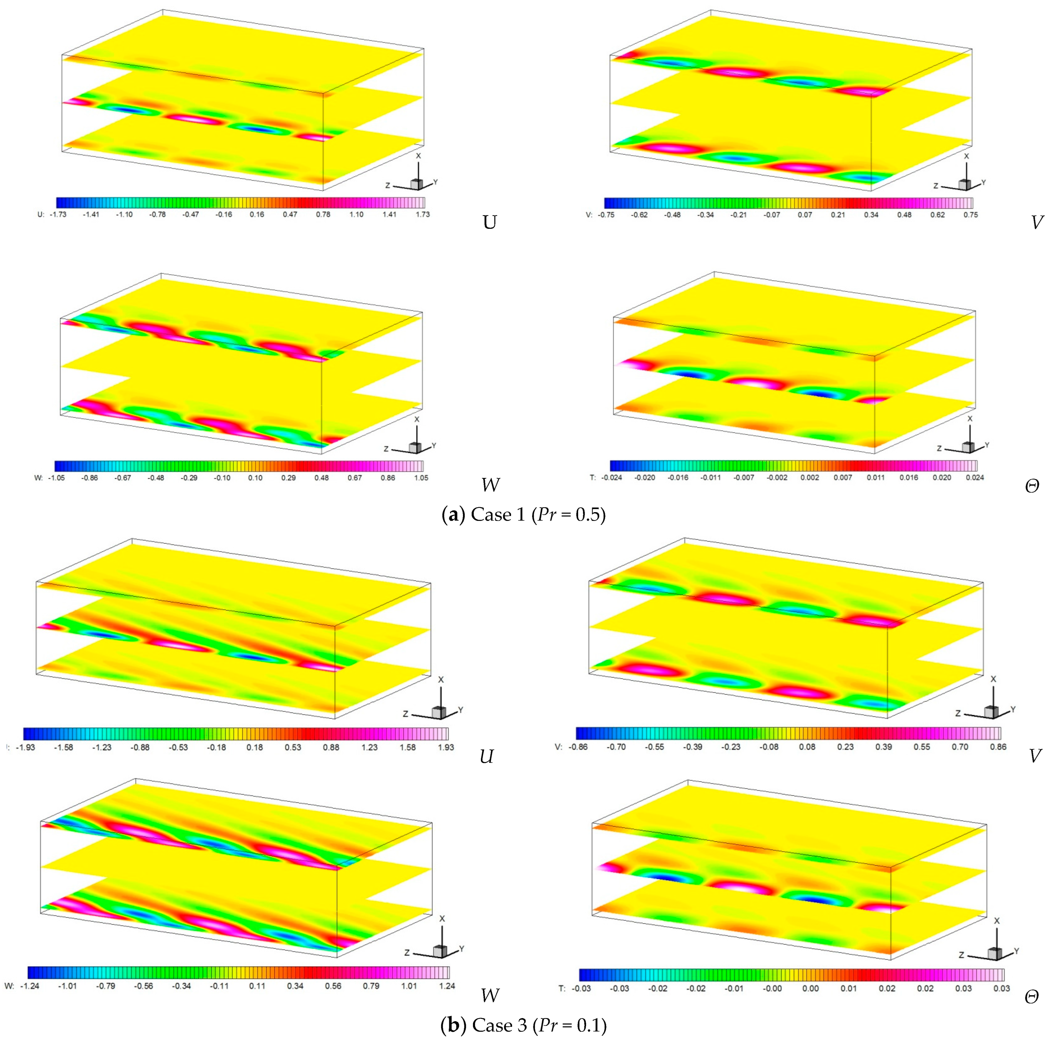
4.2.2. Effect of the Taylor Number and the Prandtl Number

In this subsection, we discuss the effects of the Taylor number and the Prandtl number. First, when the Prandtl number was fixed at 1, the calculations were performed for the three different Taylor numbers. The results are summarized in

Table 4. Effect of the Taylor number on the onset of instability at Pr = 1.

	Ta	kc	Rac	SI
Case A	105	3.82	1.1245 × 104	−1.6653 × 101
Case B	106	4.32	3.3086 × 104	−2.5993 × 101
Case C	107	4.80	1.0225 × 105	−3.5321 × 101

. It shows that the critical wavenumber, Rayleigh number and angular frequency increase with increasing the Taylor number. Compared with the critical values in Table 1, where the existence of the sidewall is not taken into account, it can be recognized that both the wavenumber and the Rayleigh number are lowered for the same Taylor number. This means that sidewall traveling-wave convection occurs at a lower Rayleigh number due to the existence of the sidewall of the container.

Figure 8 shows the contour visualization of vertical velocity and temperature at the middle horizontal cross-section for the three cases. The difference in the aspect ratio of the figure is due to the difference in the critical wavenumber. Both the velocity and the temperature disturbances are observed only near the sidewall, but they tend to become thinner as the Taylor number increases. Since S_I takes a negative value, the traveling wave has a phase velocity in the positive direction of the Z-axis. In the visualization of the vertical velocity component, a weak disturbance whose sign is opposite to that of the disturbance developed near the sidewall can also be recognized. In the temperature field, it can be seen that the disturbance is stretched obliquely backward.

We also discuss the effect of decreasing the Prandtl number.

Table 5. Effect of Prandtl number on the onset of instability at Ta = 10⁶.

	Pr	kc	Rac	SI
Case B	1	4.32	3.3086 × 104	−2.5993 × 101
Case 1	0.5	4.20	3.1615 × 104	−4.9341 × 101
Case 2	0.25	4.00	2.9227 × 104	−8.9960 × 101
Case 3	0.10	3.50	2.4580 × 104	−1.8228 × 102

summarizes the calculation results when the Taylor number is fixed at 10⁶. Numerical results were also obtained for even lower Prandtl numbers such as Pr = 0.05 and 0.025, but they are not included in Table 5. The reason for this will be explained later. As the Prandtl number decreases, the critical wavenumber and the Rayleigh number decrease, but the phase velocity increases.

Figure 9 shows the visualization of the velocity and temperature fields for Cases 1 and 3. As the Prandtl number becomes smaller, the velocity and temperature disturbances are not localized near the sidewall but spread to the bulk region. In cases such as Pr = 0.025 and 0.05, which are not listed in Table 5, a sufficiently large value of disturbance takes place even at the boundary of y = 2h. Therefore, the assumption of the sidewall traveling-wave mode fails (the computation does not diverge but it is not considered to be a physically meaningful solution). That is why Table 5 lists the results up to Pr = 0.1. From the visualization in Figure 9b, it can be observed from the W distribution that the disturbance extends diagonally forward to relatively far places from the sidewall. In the computational area with an aspect ratio of 2 (twice the container height in the Y-direction) secured in this computation, the limitation is about Pr = 0.1. This limitation value seems to depend somewhat on the Taylor number.

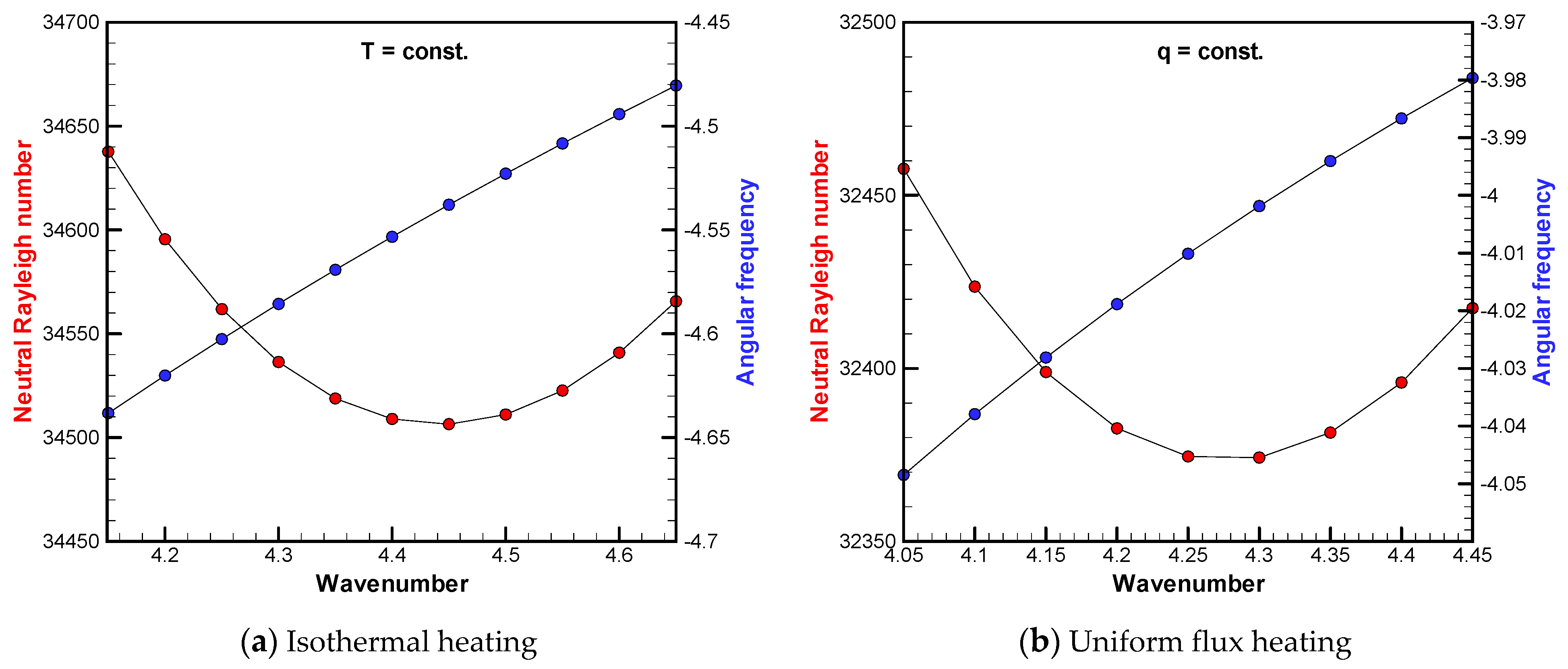
4.2.3. Effect of the Bottom Heating Condition

Figure 10 shows the neutral stability curves of the Rayleigh number and the angular frequency for the isothermal heating and the uniform flux heating. At first glance, there is not much difference due to the heating conditions of the bottom surface, and the relationships among the wavenumber, the Rayleigh number, and the angular frequency are similar to each other. The critical Rayleigh number for isothermal heating is about 34,500 at the corresponding wavenumber 4.42, while for uniform flux heating, it is about 32,370 at wavenumber 4.27. Therefore, the sidewall traveling mode occurs at a lower Rayleigh number when uniform flux heating is applied.

5. Discussion

5.1. Effect of Sidewall

As a result of performing the two-dimensional LSA including the sidewall, it was confirmed that the traveling wave occurred near the sidewall regardless of the Prandtl number. This is a phenomenon that cannot be captured by the one-dimensional LSA in which the effect of sidewalls cannot be considered. In the 1D LSA, the critical Rayleigh number for overstability was lower than that for the stationary convection, so it is predicted that oscillatory convection is more likely to occur. However, according to Chandrasekar’s studies [3,4,5], overstability does not occur above the value of Pr = 0.6766. On the other hand, in the 2D LSA considering the sidewall, a traveling wave along the sidewall was observed even when the value of the Prandtl number was larger than the critical Prandtl number of 0.6766. It is difficult to interpret the solution of overstability based on the 1D analysis as a physical phenomenon. This is because the direction of the phase velocity cannot be determined uniquely in the 1D LSA. Therefore, the 2D LSA is necessary if we need to compare it with actual experiments (which must include sidewalls).

5.2. Centrifugal Force

In the present study, we performed 2D linear stability analyses under the assumption that centrifugal force is neglected to find the critical Rayleigh number corresponding to given Taylor and Prandtl numbers, and then the velocity, temperature and the pressure fields were visualized. If the analysis takes centrifugal force into account, an additional dimensionless parameter governing this phenomenon should be considered as the Froude number, which represents the ratio of centrifugal force to gravity. In such a case, weak convection already takes place in the basic state, which is necessary for the linear stability analysis, and it is inferred that the temperature distribution deviates slightly from the heat conduction state [33]. Numerical calculations are required to obtain such a basic state. While it may be reasonable to ignore the inertia terms in the Navier–Stokes equation when attempting to obtain this weak basic flow, consideration of the convective term in the energy equation is essential. The velocity, temperature and pressure fields would change depending on the dimensionless numbers such as the Froude number and the enclosure aspect ratio. If the enclosure would have a large aspect ratio (thin fluid layer), even for a small Froude number (rotational angular velocity), the centrifugal force effect would not be negligible near the sidewall due to the large radius. When numerically calculating the basic state, it is necessary to input not only the Froude number, but also the Prandtl number (unnecessary if the inertia terms are ignored in the basic state), the Taylor number and the Rayleigh number. This is in sharp contrast to the fact that the basic state, when ignoring the centrifugal effect, is independent of dimensionless numbers. Therefore, if linear stability analysis including the centrifugal force effect is performed, it is difficult to strictly determine the neutral Rayleigh number (and thus the critical Rayleigh number). Instead, whether the weak convection caused by the combination of non-dimensional numbers input to obtain the basic state is stable or unstable can be judged by the sign of the linear growth rate obtained by the linear stability analysis.

5.3. Free-Surface

As mentioned in many textbooks, the upper and lower boundary conditions for the Rayleigh–Bénard problem consider not only solid walls but also free surfaces. In the absence of rotation, the assumption that the free surface is flat is valid, whereas in the rotating field the free surface is not flat. It is a complex problem where the free surface shape is determined by considering centrifugal force, gravity, surface tension and fluid temperature. In addition, the Marangoni effect also appears. In the analysis of phenomena with such complexities, it seems that there is not much meaning to perform such linear stability analyses anymore. Therefore, it would be preferable to execute a complete numerical simulation, although the computational cost is high. Such simulation automatically incorporates finite-amplitude nonlinear effects of disturbances.

6. Conclusions

In this study, linear stability analyses of the rotating Rayleigh–Bénard convection were carried out for cases wherein centrifugal force was ignored and the upper and lower boundary conditions were limited to solid walls. For LSA models, 1D analysis that does not consider the influence of the sidewall and 2D analysis with a vertical adiabatic sidewall were targeted.

In the 1D analysis, numerical analyses were performed for both the stationary convection mode and overstability mode, which was suggested in Chandrasekar’s study. In the stationary convection mode, the Prandtl number had nothing to do with the phenomenon, but in the overstability mode for Pr = 0.025, we confirmed quantitative agreement with Chandrasekar’s solution for a wide range of Taylor numbers.

In the 2D analysis, calculations were performed for several Prandtl numbers, limited to relatively high Taylor numbers. Within the range of parameters dealt with in the present study, we always detected the mode of the sidewall traveling wave. This mode is common to overstability in the sense that it oscillates, but it seems that the properties are different in the sense that the disturbance travels along the sidewall. It was confirmed that when the Prandtl number becomes small, the disturbance tends to spread from the sidewall to the inner bulk region.

Finally, the 2D analyses were performed when the bottom heating condition was either isothermal or uniform flux. There was a slight difference in the value of the critical Rayleigh number as well as the corresponding wavenumber. The sidewall traveling mode occurs at a lower Rayleigh number when uniform flux heating is applied.

References

1. Bénard, H. Étude expérimentale des courants de convection dans une nappe liquide.—Régime permanent: Tourbillons cellulaires. J. Phys. Théor. Appl. 1900, 9, 513–524. [Google Scholar] [CrossRef]
2. Rayleigh, L. LIX. On convection currents in a horizontal layer of fluid, when the higher temperature is on the under side. Lond. Edinb. Dublin Philos. Mag. J. Sci. 1916, 32, 529–546. [Google Scholar] [CrossRef] [Green Version]
3. Chandrasekar, S. Hydrodynamic and Hydromagnetic Stability; Dover Publication, Inc.: New York, NY, USA, 1961. [Google Scholar]
4. Chandrasekhar, S. The instability of a layer of fluid heated below and subject to Coriolis forces. Proc. R. Soc. London. Ser. A Math. Phys. Sci. 1953, 217, 306–327. [Google Scholar]
5. Chandrasekhar, S.; Elbert, D.D. The instability of a layer of fluid heated below and subject to Coriolis forces. II. Proc. R. Soc. London. Ser. A Math. Phys. Sci. 1955, 231, 198–210. [Google Scholar]
6. Kloosterziel, R.C.; Carnevale, G.F. Closed-form linear stability conditions for rotating Rayleigh-Bénard convection with rigid stress-free upper and lower boundaries. J. Fluid Mech. 2003, 480, 25–42. [Google Scholar] [CrossRef] [Green Version]
7. Zhong, F.; Ecke, R.E.; Steinberg, V. Rotating Rayleigh–Bénard convection: Asymmetric modes and vortex states. J. Fluid Mech. 1993, 249, 135–159. [Google Scholar] [CrossRef]
8. Buell, J.C.; Catton, I. Effect of rotation on the stability of a bounded cylindrical layer of fluid heated from below. Phys. Fluids 1983, 26, 892–896. [Google Scholar] [CrossRef]
9. Ning, L.; Ecke, R.E. Rotating Rayleigh-Bénard convection: Aspect-ratio dependence of the initial bifurcations. Phys. Rev. E 1993, 47, 3326. [Google Scholar] [CrossRef] [Green Version]
10. Liu, Y.; Ecke, R.E. Nonlinear traveling waves in rotating Rayleigh-Bénard convection: Stability boundaries and phase diffusion. Phys. Rev. E 1999, 59, 4091. [Google Scholar] [CrossRef]
11. Kuo, E.Y.; Cross, M.C. Traveling-wave wall states in rotating Rayleigh-Bénard convection. Phys. Rev. E 1993, 47, R2245. [Google Scholar] [CrossRef] [Green Version]
12. Herrmann, J.; Busse, F.H. Asymptotic theory of wall-attached convection in a rotating fluid layer. J. Fluid Mech. 1993, 255, 183–194. [Google Scholar] [CrossRef]
13. Goldstein, H.F.; Knobloch, E.; Mercader, I.; Net, M. Convection in a rotating cylinder. Part 1 Linear theory for moderate Prandtl numbers. J. Fluid Mech. 1993, 248, 583–604. [Google Scholar] [CrossRef]
14. Goldstein, H.F.; Knobloch, E.; Mercader, I.; Net, M. Convection in a rotating cylinder. Part 2. Linear theory for low Prandtl numbers. J. Fluid Mech. 1994, 262, 293–324. [Google Scholar] [CrossRef] [Green Version]
15. Bajaj, K.M.; Ahlers, G.; Pesch, W. Rayleigh-Bénard convection with rotation at small Prandtl numbers. Phys. Rev. E 2002, 65, 056309. [Google Scholar] [CrossRef] [Green Version]
16. Plaut, E. Nonlinear dynamics of traveling waves in rotating Rayleigh-Bénard convection: Effects of the boundary conditions and of the topology. Phys. Rev. E 2003, 67, 046303. [Google Scholar] [CrossRef] [PubMed]
17. Scheel, J.D. The amplitude equation for rotating Rayleigh–Bénard convection. Phys. Fluids 2007, 19, 104105. [Google Scholar] [CrossRef]
18. Tagare, S.G.; Babu, A.B.; Rameshwar, Y. Rayleigh–Benard convection in rotating fluids. Int. J. Heat Mass Transf. 2008, 51, 1168–1178. [Google Scholar] [CrossRef]
19. Husain, A.; Baig, M.F.; Varshney, H. Turbulent rotating Rayleigh–Benard convection: Spatiotemporal and statistical study. J. Heat Transf. 2009, 131, 022501. [Google Scholar] [CrossRef]
20. Yu, J.; Goldfaden, A.; Flagstad, M.; Scheel, J.D. Onset of Rayleigh-Bénard convection for intermediate aspect ratio cylindrical containers. Phys. Fluids 2017, 29, 024107. [Google Scholar] [CrossRef]
21. Favier, B.; Guervilly, C.; Knobloch, E. Subcritical turbulent condensate in rapidly rotating Rayleigh–Bénard convection. J. Fluid Mech. 2019, 864, R1. [Google Scholar] [CrossRef] [Green Version]
22. Favier, B.; Knobloch, E. Robust wall states in rapidly rotating Rayleigh–Bénard convection. J. Fluid Mech. 2020, 895, R1. [Google Scholar] [CrossRef]
23. Vishnu, V.T.; De, A.K.; Mishra, P.K. Dynamics and statistics of reorientations of large-scale circulation in turbulent rotating Rayleigh-Bénard convection. Phys. Fluids 2019, 31, 055112. [Google Scholar] [CrossRef] [Green Version]
24. Noto, D.; Tasaka, Y.; Yanagisawa, T.; Murai, Y. Horizontal diffusive motion of columnar vortices in rotating Rayleigh–Bénard convection. J. Fluid Mech. 2019, 871, 401–426. [Google Scholar] [CrossRef] [Green Version]
25. Shi, J.Q.; Lu, H.Y.; Ding, S.S.; Zhong, J.Q. Fine vortex structure and flow transition to the geostrophic regime in rotating Rayleigh-Bénard convection. Phys. Rev. Fluids 2020, 5, 011501. [Google Scholar] [CrossRef] [Green Version]
26. Maffei, S.; Krouss, M.J.; Julien, K.; Calkins, M.A. On the inverse cascade and flow speed scaling behaviour in rapidly rotating Rayleigh–Bénard convection. J. Fluid Mech. 2021, 913, A18. [Google Scholar] [CrossRef]
27. Guzmán, A.J.A.; Madonia, M.; Cheng, J.S.; Ostilla-Mónico, R.; Clercx, H.J.; Kunnen, R.P. Force balance in rapidly rotating Rayleigh–Bénard convection. J. Fluid Mech. 2021, 928, A16. [Google Scholar] [CrossRef] [PubMed]
28. Cai, T. Large-scale Vortices in rapidly rotating Rayleigh–Bénard convection at small Prandtl number. Astrophys. J. 2021, 923, 138. [Google Scholar] [CrossRef]
29. Ecke, R.E. Rotating Rayleigh-Bénard convection: Bits and pieces. Phys. D Nonlinear Phenom. 2022, 444, 133579. [Google Scholar] [CrossRef]
30. Ecke, R.E.; Zhang, X.; Shishkina, O. Connecting wall modes and boundary zonal flows in rotating Rayleigh-Bénard convection. Phys. Rev. Fluids 2022, 7, L011501. [Google Scholar] [CrossRef]
31. Tagawa, T. Linear stability analysis of liquid metal flow in an insulating rectangular duct under external uniform magnetic field. Fluids 2019, 4, 177. [Google Scholar] [CrossRef] [Green Version]
32. Tagawa, T. Effect of the direction of uniform horizontal magnetic field on the linear stability of natural convection in a long vertical rectangular enclosure. Symmetry 2020, 12, 1689. [Google Scholar] [CrossRef]
33. Satake, H.; Tagawa, T. Influence of centrifugal buoyancy in thermal convection within a rotating spherical shell. Symmetry 2022, 14, 2021. [Google Scholar] [CrossRef]
Figure 1. Schematic illustration of the rotating Rayleigh–Bénard convection. The black arrows indicate the wave-like velocity vectors that are formed near the sidewalls, and they travel along the sidewall in clockwise direction.
Fluids 08 00096 g001
Figure 2. Visualization of eigenfunctions for a wavelength for stationary convection at the critical state of k = 4.8, Ra = 4.71 × 10³ and Ta = 104.
Fluids 08 00096 g002
Figure 3. Neutral stability curve of the Rayleigh number near the critical point and the angular frequency for Pr = 0.025 and Ta = 106.
Fluids 08 00096 g003
Figure 4. Visualization of eigenfunctions within the fluid layer for a wavelength for overstability at the critical state of Pr = 0.025, k = 4.09, Ra = 9.51 × 10³ and Ta = 106.
Fluids 08 00096 g004
Figure 5. Neutral stability curve of the Rayleigh number near the critical point and the angular frequency for Pr = 6.3 and Ta = 3 × 10⁵.
Fluids 08 00096 g005
Figure 6. Grid dependency for the three systems. Contour maps of the real part of vertical velocity component (left) and the real part of the pressure (right) at the neutral state for k = 4.225, Pr = 6.3 and Ta = 3 × 10⁵.
Fluids 08 00096 g006
Figure 7. Isosurface of the eigenfunctions for two wavelengths at the critical state of Ra = 19649, k = 4.225, Pr = 6.3 and Ta = 3 × 10⁵.
Fluids 08 00096 g007
Figure 8. Contour maps of the vertical velocity component (left) and the temperature (right) for two wavelengths at the X = 0.5 cross-section for Pr = 1.0.
Fluids 08 00096 g008
Figure 9. Contour maps of the three velocity components (U, V, W), and the temperature (Θ) for two wavelengths at the X = 0.1, 0.5 and 0.9 cross-sections for Ta = 106.
Fluids 08 00096 g009
Figure 10. Neutral stability curve of the Rayleigh number near the critical point and the angular frequency at Pr = 6 and Ta = 106.
Fluids 08 00096 g010