1. Introduction
The change in the qualitative state of the raw material base leads to development and involvement in the operation of oil fields with high contents of paraffins, resins, and asphaltenes. The development of such deposits requires the use of unconventional methods of oil production and its preparation for transportation. Light oil products (gasoline, kerosene, etc.) are easily transported through pipelines at any time of the year and operations with them do not cause any particular difficulties. The operations with dark oil products (fuel oil, lubricating oils, etc.) and crude oil cause significant difficulties due to the fact that dark oil products become more viscous when the air temperature drops, and their transportation without heating becomes impossible. For the pipeline transportation of oil and oil products, an approach is used based on the regulation of the rheological properties of oil, for example, by heating the oil with its subsequent transportation through a pipeline with increased thermal insulation (hot oil transfer). In some cases, an increase in the viscosity of oil with a decrease in temperature leads to unacceptable stresses on the walls of the pipeline and stops transportation.
Heat exchange processes are carried out in heat exchangers of various types and designs [
1,
2,
3,
4,
5]. For heating, various heat carriers are used, for example, hot water or steam. Energy consumption is one of the important factors that has a significant impact on the choice of heat exchanger design [
6]. In the oil and gas industry, shell and tube heat exchangers are used, which provide good performance characteristics over a wide range of operating conditions, high reliability, and low cost. To determine the efficiency of heat exchange processes, final temperatures and the required operating parameters of heat carriers, a thermal calculation is performed.
The composition of oil (in particular, the content of asphaltenes, resins, and paraffins) has a significant effect on the dependence of viscosity on temperature [
7,
8]. Empirical formulas describing the change in kinematic viscosity depending on temperature have the form of various functions (exponential, polynomial, power, etc.), which are characterized by the presence of coefficients that depend on the properties of the liquid. Constant coefficients are determined based on measurements of kinematic viscosity at several points. To calculate the thermodynamic parameters of oil, gas condensates, and their fractions, the generalized Lee–Kessler equation of state [
9] is used. The dependence of the kinematic viscosity of oil and oil mixtures on temperature is analysed in [
10], where the existing formulas for calculating the kinematic viscosity of oil in main pipelines are compared.
The fluid flow in the annular space of the heat exchanger is complex and depends on many factors. The numerical modelling of heat transfer in heat exchange devices of various designs is carried out in [
11,
12]. The results of the numerical calculations are used to find the optimal ways to intensify heat transfer processes [
13,
14,
15]. The results obtained indicate a decrease in the effect of the viscosity of the pumped oil on the hydraulic characteristics of the pipeline when pumping in developed turbulent regimes.
A comparison of the accuracy of various turbulence models used to close the Reynolds-averaged Navier–Stones (RANS) equations is the subject of study in [
16,
17,
18,
19]. Two-parameter turbulence models, including the
k–
model,
k–
model, and SST model, are used in the CFD calculations. The obtained results are in satisfactory agreement with the data of the industrial experiments. This allows for solving the problems of process control and increasing production efficiency and determining the optimal regime parameters of technological processes. At the same time, the available calculations using two-parameter turbulence models do not take into account the laminar–turbulent transition, which affects the determination of the effective length of the heat exchanger.
Many experimental and computational works have been performed before, and various flow arrangements and methods of enhancement of heat transfer have been proposed and investigated [
20,
21,
22,
23]. In classical heat exchangers, a tube bundle for one coolant is placed inside a casing along which another coolant moves. In the design of helicoid heat exchangers, profiled tubes and screw profile fins are used, with the help of which heat exchange conditions are improved. The tubes have a small diameter and thin walls (about 0.3 mm). In the case where the viscosity depends on temperature, the flow regime in such thin tubes changes from laminar to turbulent.
Reducing the viscosity of oil by heating it is one of the ways to increase the energy efficiency of the process of pumping high-viscosity oil during production and transportation. Performing numerical simulation allows for solving a number of issues related to improving the efficiency of heat transfer, which remains one of the most important in the design of heat exchange devices in the oil and gas industry. The laminar–turbulent transition plays a significant role in a new type of heat exchangers, for example, helicoid ones, consisting of a large number of long thin profiled tubes and being characterized by a high speed of the heat carriers used. In this study, a mathematical model of a heat exchanger is developed that takes into account the laminar–turbulent transition. For simplicity, a “pipe in pipe” heat exchanger scheme with a thin and smooth inner tube is selected. A calculation method is provided for a parallel flow heat exchanger, in which the working fluid in the inner pipeline is oil (cold coolant), and, in the outer pipe, it is water (hot coolant). The calculations are carried out for a model design of a heat exchanger both using a theoretical approach based on the Log–Mean Temperature Difference (LMTD) method at constant and variable viscosity, and based on Computational Fluid Dynamics (CFD) tools. The data obtained within the framework of various approaches are compared with each other, which causes it to be possible to draw a conclusion about the accuracy of each of the approaches and the possibility of their application in practice.
2. Dependence of Viscosity on Temperature
The Uzen oil and gas field is located in the Mangistau region of Kazakhstan. The oil deposits are deep 0.9–2.4 km. The oil density is 844–874 kg/m3, dynamic viscosity is 3.4–8.15 mPa·c, content of sulphur is 0.16–2%, content of paraffins is 16–22%, and content of resins is 8–20%.
In the literature, various formulas are used to take into account the dependence of viscosity on temperature. In the oil industry, temperature-dependent kinematic viscosity, the Walther formula is widely used [
10]:
where
a and
b are empirical coefficients experimentally determined. The coefficients
a and
b in the Formula (
1) are found from the relations
Here, and are kinematic viscosity values at temperatures and .
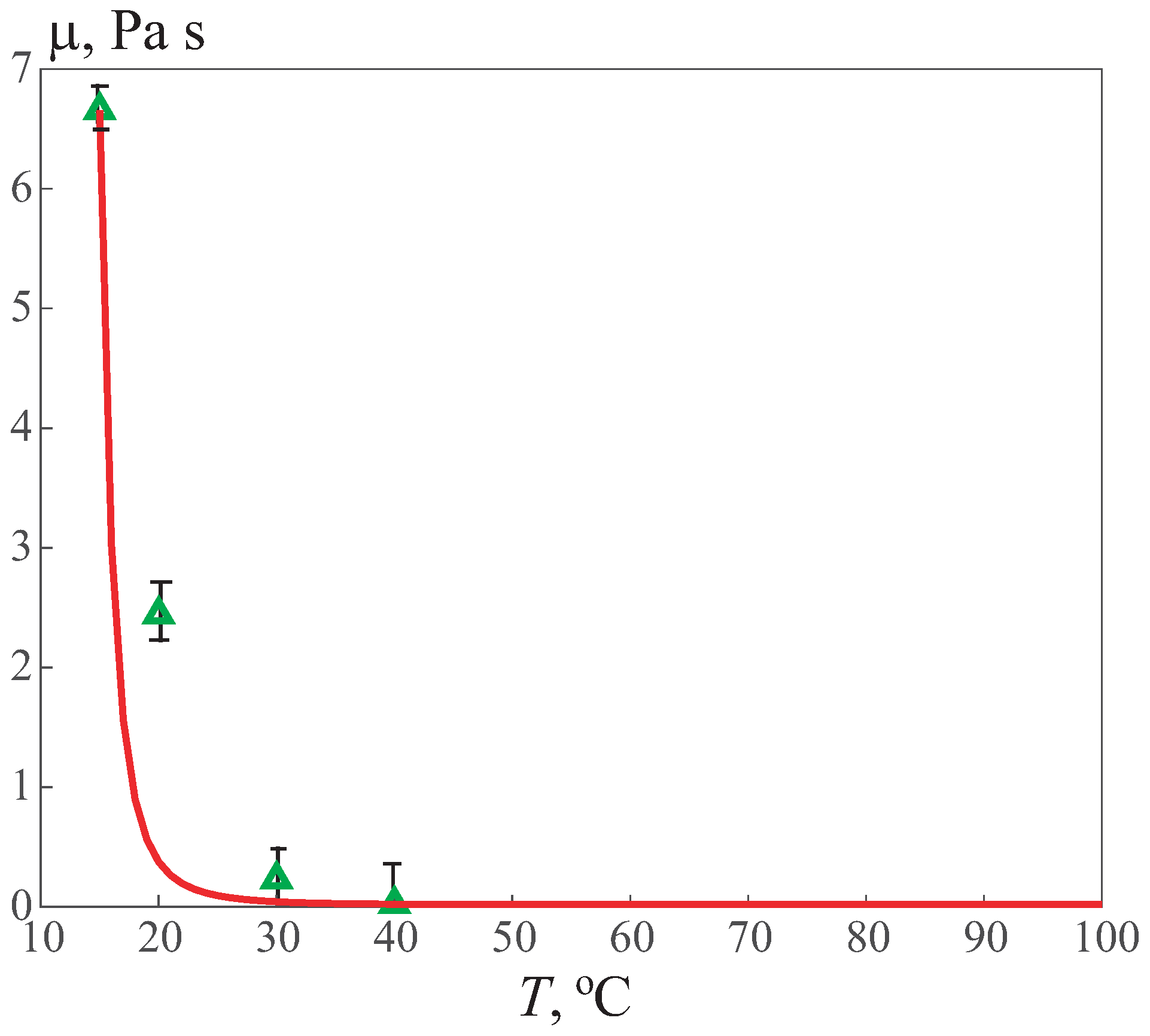
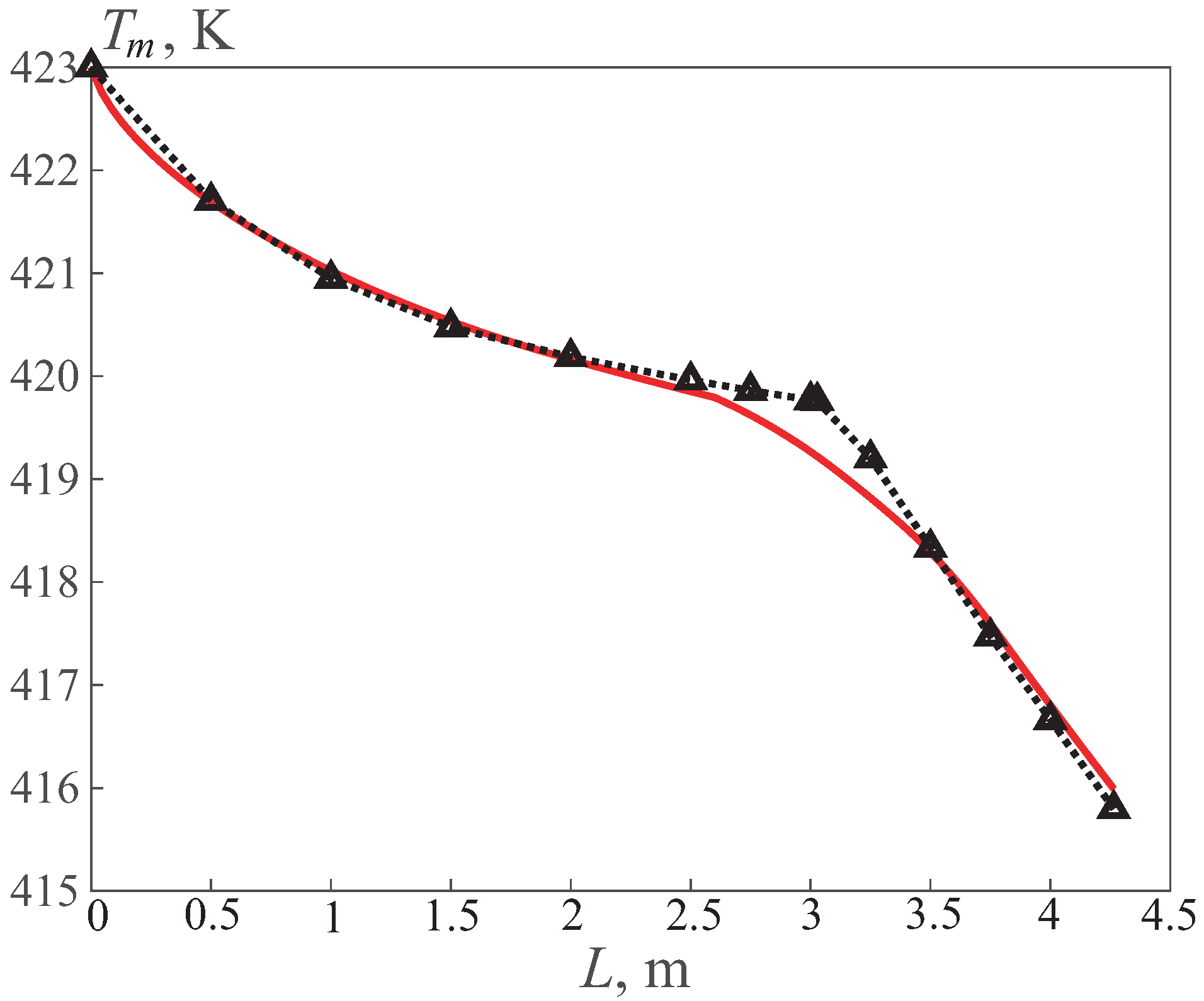
The comparison of the results of calculations using the Voltaire formula with the experimental values of dynamic viscosity is shown in
Figure 1 for oil from the Uzen field. The solid line corresponds to the dependence of the viscosity on temperature, obtained using the Walther Formula (
1), and the triangular icons correspond to the results of a physical experiment [
24].
The rheological properties of oil are considered as a property of a colloidal and dispersed system, which, under certain conditions, is prone to the formation of bulk structures with pronounced thixotropy. The rheological parameters of oil are experimentally estimated by the nature of the dependence of shear stresses on the shear gradient.
In a state of equilibrium, the oil system behaves similar to a plastic fluid and has some spatial structures that can resist shear stress until its value exceeds the value of the static shear stress. After reaching a certain shear rate, the oil is able to flow as a Newtonian fluid. An example of a plastic fluid are oils with a high paraffin content at temperatures below the crystallization temperature, abnormally viscous oils, with a high content of asphaltenes, and structured colloidal systems used for enhanced oil recovery.
The viscosity of Newtonian oil does not depend on the deformation mode and is constant. Such oil is characterized by a relatively low content of resins, mainly not exceeding 15–20%. The oils with a low content of high-melting paraffins, as a rule, do not form structures and are classified as Newtonian liquids. For non-Newtonian oil, the viscosity during movement changes with time, since the destruction of the spatial structure is constantly occurring. The structural and mechanical properties of non-Newtonian oil disappear when heated.
The properties of oil from the Uzen field allow it to be attributed to Newtonian fluids. The Newtonian model can be used as a basis for research. This is all the more true for the use of various turbulence models, which, as a rule, are tested on a number of problems for media exhibiting Newtonian properties.
3. Method for Constant Viscosity
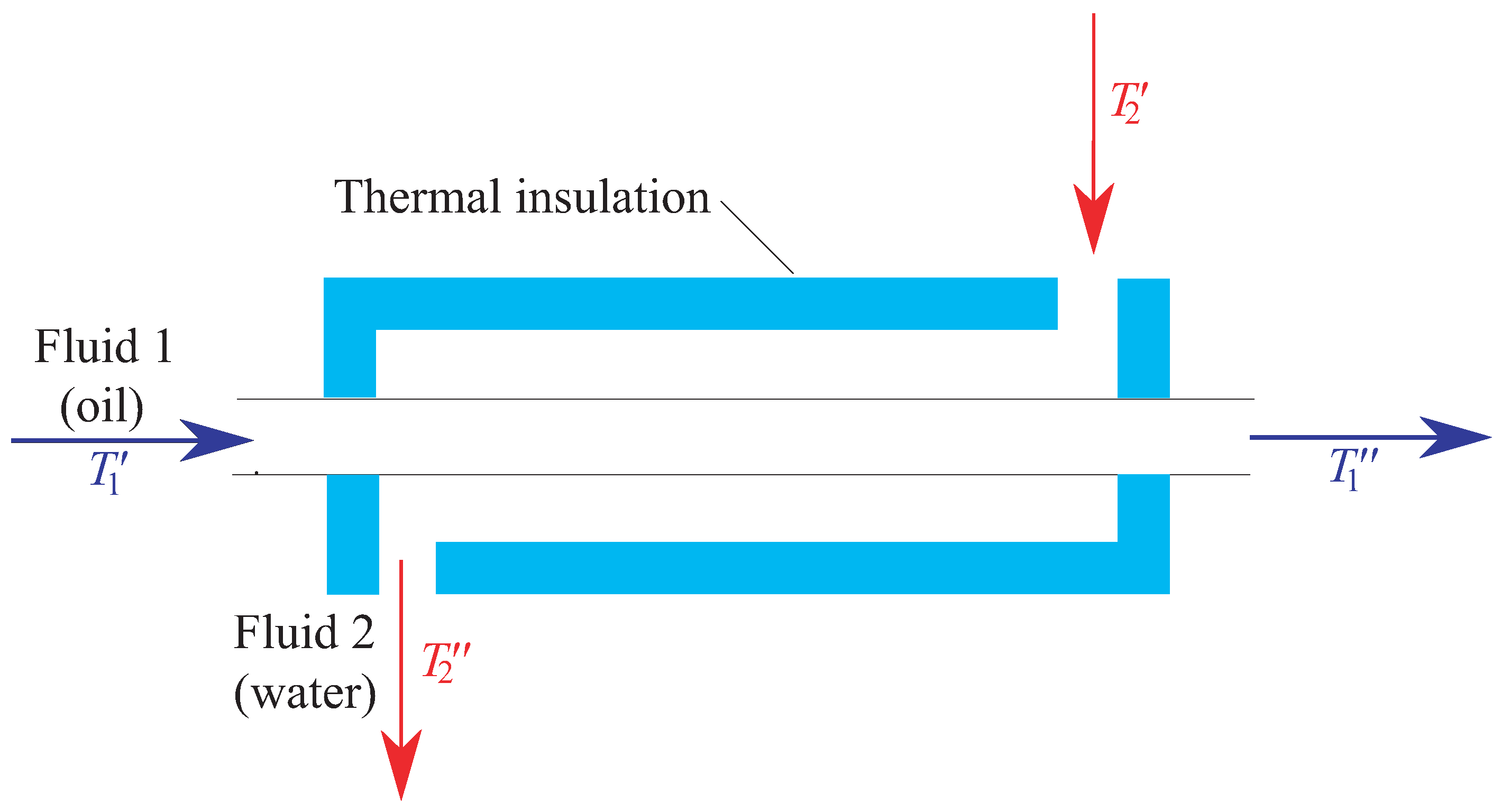
To estimate heat flux from a hot coolant to a cold coolant, a model of a coolant with a constant viscosity along the length is used, based on the use of the log–mean temperature difference. In a recuperative heat exchanger, two fluids with different temperatures move in a space separated by a solid wall (
Figure 2). The thermal calculation is reduced to the coupled solution of the equations of the heat balance and heat transfer.
The energy balance equation has the form [
25]:
Here, Q is amount of heat transferring from hot stream to cold stream, G is the mass flow rate, is the specific heat capacity, is the inlet temperature, and is the outlet temperature. Subscript 1 corresponds to the hot stream, and subscript 2 corresponds to the cold stream.
The heat transfer equation for a heat exchanger is represented as
where
is the average heat transfer coefficient calculated at average temperature
and
,
is the average temperature difference. The average temperature difference is defined as
where
F is the surface area.
Defining
, Equations (
2) and (
3) are written in differential form:
The plus sign is chosen in the case of a parallel heat exchanger, and the minus sign is chosen in the case of a counterflow heat exchanger. The equation is valid along the direction of movement of the hot stream. Assuming that
m and
are constant over the length, integration from 0 to
F and from
and
leads to the equation
where
is temperature difference at the inlet of the hot coolant. The temperature difference along the heat exchange surface changes exponentially. By averaging the temperature difference over the entire heat exchange surface, the logarithmic mean temperature difference is found from the relation
In the design calculation of heat exchanges, the amount of heat
Q is determined using Equation (
2). The area of the heat exchange surface
F is found from the equation
When calculating the heat transfer surface area, the problem is reduced to calculating the average heat transfer coefficient and the logarithmic mean temperature difference. The length of the heat exchange device is calculated using the formula , where n is number of inner tubes and d is their hydraulic diameter.
The temperature distributions along the heat exchange surface are expressed by the relations:
- —
Parallel flow heat exchanger:
- —
Counterflow heat exchanger:
Here, is the dependence of the heat exchange surface area on the length measured along the path of the hot coolant. In the case of a cylindrical surface, the heat transfer area is expressed in terms of the length , where is the wetted perimeter heat exchange surfaces.
For the case of thin cylindrical walls, the relations for surface temperatures have the form
Here, , is the heat exchange area from coolant 1 side, is the heat transfer area from coolant 2 side, is the thickness wall, is the thermal conductivity of the wall, and is the heat transfer coefficient. The relations are implicit and require an iterative solution, since the heat transfer coefficient depend on the temperature.
For a thin single-layer wall, the average heat transfer coefficient is calculated as follows
where
is average heat transfer coefficient to the cold coolant and
is average heat transfer coefficient to the hot coolant.
The Nusselt number depends on the flow regime (laminar or turbulent) and the heat transfer regime (heating or cooling). The average heat transfer coefficient is expressed in terms of the Nusselt number averaged over the length
, where
is the effective hydraulic diameter,
is the flow area channel,
is the wetted perimeter, and
is the liquid thermal conductivity. For the flow in a pipe or for the longitudinal flow around bundles of pipes, the Nusselt number is calculated using a semi-empirical dependence of the form
where
is the Reynolds number,
is the Prandtl number, and
is the Prandtl number calculated at the wall temperature. The similarity numbers are calculated from the average coolant temperature. The Reynolds number is defined as
, where
v is the characteristic flow velocity,
is the density, and
is the dynamic viscosity.
4. Method for Variable Viscosity
In the case of a strong dependence of viscosity on temperature, the heat exchanger is divided into elementary sections along the length. At each section, an assumption is presented about a negligible change in the viscosity. The local Nusselt numbers in the laminar and turbulent flow regimes are found using semi-empirical relations. The transition between different criterion relationships corresponding to laminar, transitional, and turbulent flow regimes is realized depending on the Reynolds number.
With a weak dependence of the viscosity of the coolant on temperature, the average Reynolds number is found from the average temperature of the coolant. Such an assumption does not introduce significant errors into the calculation, since it practically does not affect the flow regime. In the case of a strong dependence of viscosity on temperature, as the coolant heats up, the flow regime changes from laminar to developed turbulent. In this case, the local heat transfer coefficient
is calculated, and the relations for the local Nusselt number
calculated from local similarity numbers are used
The average value of the heat transfer coefficient is found using the formula
To calculate the local Nusslelt number in the laminar flow regime in a pipe (for
), the following relation is used [
25]:
This relation is valid for
. The expression for calculating the local Nusselt number for the turbulent flow in a pipe (for
) with an additional correction for the change in the Prandtl number has the form
where
In the transient flow regime, linear interpolation is used. For an annular channel in a turbulent flow regime, the ratio is used as for the flow in a pipe but with its own equivalent hydraulic diameter.
The heat balance equation for an elementary section in the direction of movement of the hot coolant is written in the following form
Here,
is the loss of the heat quantity by the hot coolant,
is the acquired quantity of heat by the cold coolant,
G is the mass flow rate of the coolant,
is the heat capacity, and
is the temperature change. The plus sign corresponds to the direct-flow circuit and the minus sign corresponds to the counterflow circuit. The heat transfer equation for an elementary section adopts the form
Here, k is the local heat transfer coefficient and is the change in the heat exchange area, which remains constant for a heat exchanger of straight pipes.
Equations (
5) and (
6) imply a closed system of equations for coolant temperatures
Since
is known, the system of Equation (
7) is a system of ordinary differential equations with a non-linear right-hand side. In the case of a direct-flow scheme (plus sign), the Cauchy problem is posed for the system (
7), and, for a counterflow scheme (minus sign), a boundary value problem is solved. In this case, the integration is carried out up to the length
L, which is not known in advance.
The system of Equation (
7) is solved by the finite difference method on the interval
, which causes it to be possible to apply the developed approach for calculating both the direct-flow and counter-flow heat exchangers. To stabilize the iterative process during the linearization of the system, the under-relaxation method is used. The length of the integration interval
L is not known in advance. Newton’s method is used to determine it.
5. CFD Simulation
The results of the thermal calculations are compared with the data obtained using the CFD methods. Oil is considered a Newtonian fluid with a constant density. The calculations are carried out using the numerical solution of the RANS equations for a viscous incompressible fluid, closed using a turbulence model that takes into account the laminar–turbulent transition.
The numerical simulation of fluid flow and heat transfer includes the numerical solution of continuity, momentum, and energy transport equations in the computational domain. The flow is described in the Cartesian coordinates. The governing equations for steady state flow have the form:
- —
Momentum equation:
- —
Energy equation:
Here, is the density and is the velocity component in the coordinate direction. p is the pressure, T is the temperature, is the kinematic viscosity, and Pr is the Prandtl number. Subscript t corresponds to the turbulent flow quantities. For a simulation of the turbulent flows, the linear model employs a Boussinesq stress–strain relation. The eddy viscosity is found from the solution of the transport equations of the turbulence model. Water and oil are Newtonian incompressible fluids. It is assumed for simplicity that water and oil satisfy the equation of the state of ideal gas with their densities.
The turbulence models that are usually used in the CFD simulations of internal and external flows do not take into account the laminar–turbulent transition. In some turbulence models, a transition point is predicted before the calculations based on some additional considerations. In the analysis of the CFD results, a flow transition from the laminar regime to the turbulent is defined using a distribution of the skin friction coefficient. However, this way is not accurate and could not be applied to a wide range of practical applications. There are a limited number of turbulence models taking into account the laminar–turbulent transition.
The SST turbulence model is designed to efficiently combine the reliable
k–
model in the near-wall region and
k–
model in free flow [
26,
27]. To switch between models, a special function is used that removes a unit value in the near-wall region (the standard
k–
model is used) and a zero value away from the wall (the
k–
model is used).
The model that takes into account the laminar–turbulent transition (Local-Correlation Transition Model,
–
transition model) is based on a combination of the equations of the SST turbulence model with two additional transport equations for the intermittency parameter
and the critical Reynolds number
constructed from the momentum loss thickness [
28,
29].
The turbulence model, proposed in [
28], includes solutions for two extra transport equations. One equation is written for the transition onset momentum thickness Reynolds number,
(it is included into the correlation between the location of the transition onset and transition location), and the other equations is derived for the intermittency,
(measure of the flow regime). The transport equations for the momentum thickness Reynolds number and intermittency have the form:
- —
Equation for momentum thickness Reynolds number:
- —
Equation for intermittency:
Here, is the production term of the momentum thickness Reynolds number, and are production and dissipation terms of the intermittency, and are constants of the model.
The mass flow rate is specified in the inlet section of the tube, and the free outflow boundary conditions are applied to the outlet section. The external tube is considered as perfectly insulated with the specification of the adiabatic boundary conditions on the solid wall.
To simplify the model, the equation for
is not considered, and the equation for the intermittency parameter assumes that the convective terms are small [
30]. This approach leads to algebraic relations for finding the intermittency parameter. The
–
model used in the calculations was developed to solve problems in the external aerodynamics. Subsequently, the model was used to simulate a wide range of flows. In particular, [
31] compared different turbulence models (
k–
,
k–
,
k–
SST,
–
f,
–
) applied to the flow in the channel.
To discretize the governing Equations (
8)–(
12), the finite volume method on unstructured meshes is used [
32]. The computational procedure employs the time marching algorithm. Time integration is carried out by the third order Runge–Kutta method. The inviscid fluxes are discretized using the MUSCL (Monotonic Upstream Schemes for Conservation Laws) scheme, and the viscous fluxes are discretized using a centred scheme of the second order. The MUSCL scheme causes it to be possible to increase the order of approximation in the spatial variables without losing the monotonicity of the solution, satisfies the TVD (Total Variation Diminishing) condition, and is a combination of the centred finite differences of the second order and a dissipative term, which are switched between using a flux limiter built on the basis of characteristic variables. The geometric multigrid method [
33] is used to solve the system of difference equations.
The energy balance equation for the solid domain is written as
where
is the density,
c is the specific heat capacity, and
is the thermal conductivity. The internal heat sources in Equation (
13) are neglected.
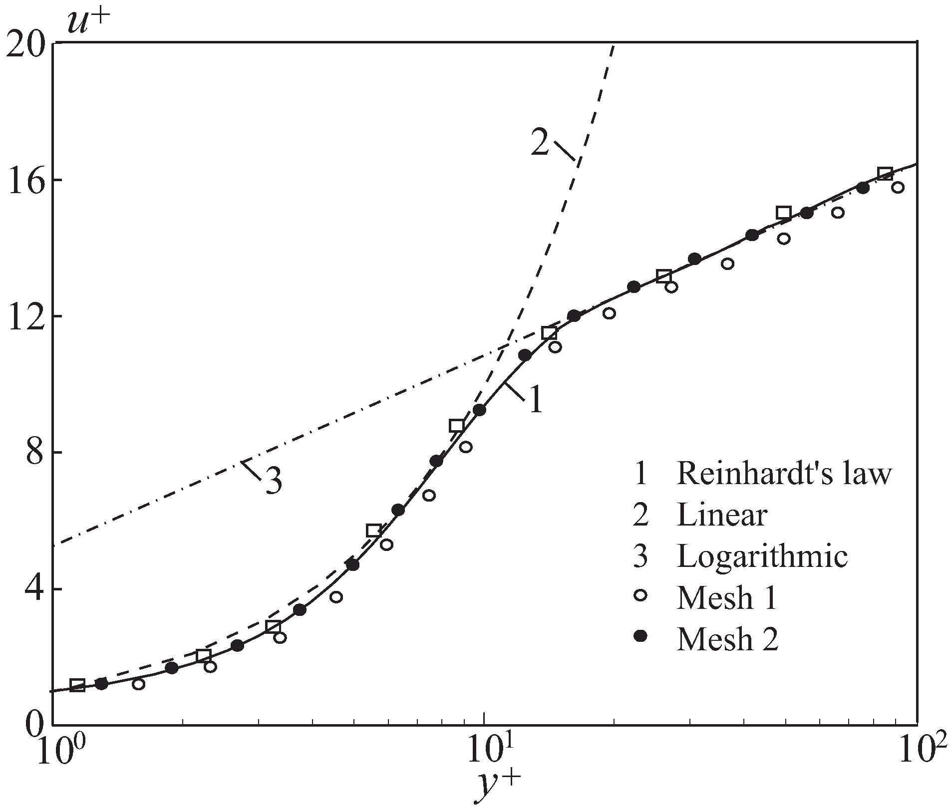
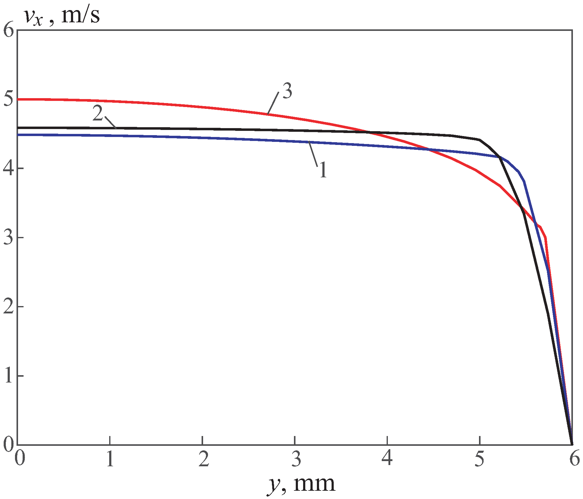
To perform mesh sensitivity analysis, the boundary layer velocity profiles computed with various meshes are assessed. The comparison of the velocity profiles is presented in
Figure 3. The Reinhard’s law covering the boundary layer region (line 1), linear (line 2), and logarithmic (line 3) velocity profiles are also presented. The symbols □, •, and ∘ correspond to meshes with 12 (mesh 1), 24 (mesh 2), and 48 (mesh 3) nodes in the normal direction (the number of nodes in a stream-wise directions is the same for the three meshes). The results obtained show that the velocity profiles computed with meshes 2 and 3 are similar and the maximum discrepancy between them is not larger than 3%. Mesh 2 is used in the CFD simulations.
The calculations use a mesh consisting of 19,461 cells, of which
cells are placed in the area filled with oil,
cells are placed in the steel area, and
cells are placed in an area filled with water (
Figure 4). The cells are thickened near the pipe walls in such a way that
, where
is the dimensionless near-wall coordinate. To achieve this, 15 mesh nodes are placed in the near-wall layer; the distance between varies according to the law of geometric progression.
To control the convergence of the iterative process, the discrepancy level of the unknown physical quantities and satisfying of the mass balance equation are verified. The calculations are terminated when the level of discrepancy of all the physical quantities decreases by three orders of magnitude, and the mismatch of the mass flow rates at the input and output boundaries of the computational domain becomes less than kg/s.
6. Results and Discussion
The forward flow scheme was chosen as a model. The developed approach does not impose restrictions on the scheme of the heat exchanger used. For the ordinary differential equations with constant or variable viscosity, the Cauchy problem is not solved (which is obtained only with the parallel flow scheme) but the boundary value problem (in the case of the parallel flow scheme, the boundary conditions are set at one end, and, in the counterflow scheme, the boundary conditions are specified at different ends of the pipes).
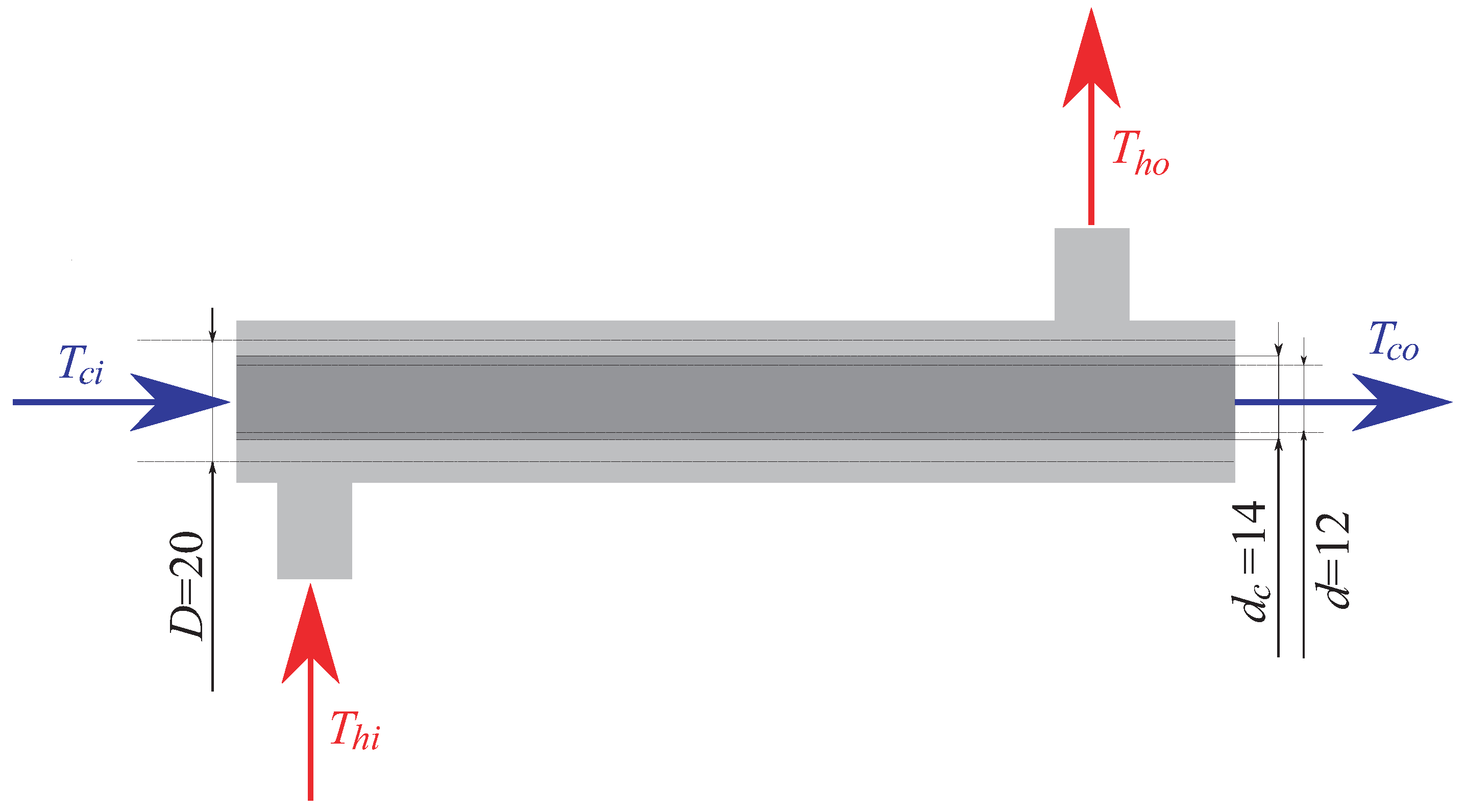
Figure 5 shows the diagram of a parallel flow heat exchanger (the dimensions are provided in millimetres). The index
h corresponds to a hot medium (water) and the index
c corresponds to a cold medium (oil). The indices
i and
o refer to the inlet and outlet sections.
To calculate the effective length of the heat exchanger and the temperature of the hot heat carrier at the outlet, the parameters provided in
Table 1 are specified (inlet and outlet temperatures of the cold heat carrier, inlet temperature of the hot and outer tubes, and the physical properties of the tube material).
To calculate the effective length of the heat exchanger and the temperature of the hot coolant at the outlet, the following parameters are set: K and K (inlet and outlet temperatures of the cold coolant), K (hot coolant inlet temperature), m/s and m/s (cold and hot coolant velocities), kg/s and kg/c (mass flow rates of hot and cold coolant), geometric characteristics (tube wall thickness mm, inner and outer diameters of tubes mm and mm, casing inner diameter mm), and the physical properties of the tube material. The transitions between different semi-empirical Equations (laminar, transient, and turbulent) are implemented by a jump based on the Reynolds number calculated from the average mass velocity.
The heat balance equations are used to determine the hot outlet temperature and the corresponding effective length of the heat exchanger. Solving the heat balance equations using the finite difference method, the distributions of the mass–average coolant temperatures provided in
Table 2 are obtained. Solving the heat balance equations by the finite difference method, the length of the heat exchanger is
m in the case of the constant viscosity and the length of the heat exchanger is
in the case of the variable viscosity. In both cases, the temperature of the hot coolant at the outlet reaches 416 K.
The results obtained are compared with the CFD data.
Figure 6 shows the distributions of the mass–average temperature of oil (cold coolant) along the length of the heat exchanger, obtained using the finite difference method and based on the numerical simulation. The mass–average oil temperature increases along the length due to heating from a heat source (hot coolant). The results of the theoretical and numerical calculations are in good agreement with each other.
The distributions of the mass–average temperature of water (hot coolant) along the length, obtained on the basis of theoretical and numerical calculations, are shown in
Figure 7. Compared to the results shown in
Figure 6, the mass–average water temperature decreases along the length due to the heat transfer from it to the cold coolant. It should also be noted that there is a good agreement between the results of the calculations obtained on the basis of different approaches.
From the results shown in
Figure 6 and
Figure 7, one can notice the characteristic changes in the curvature of the lines at a distance of about 2.5 m from the inlet section, where, in both cases, there are sharp changes in the temperature gradients with the corresponding signs. This transition occurs at the distance where the laminar flow regime becomes turbulent.
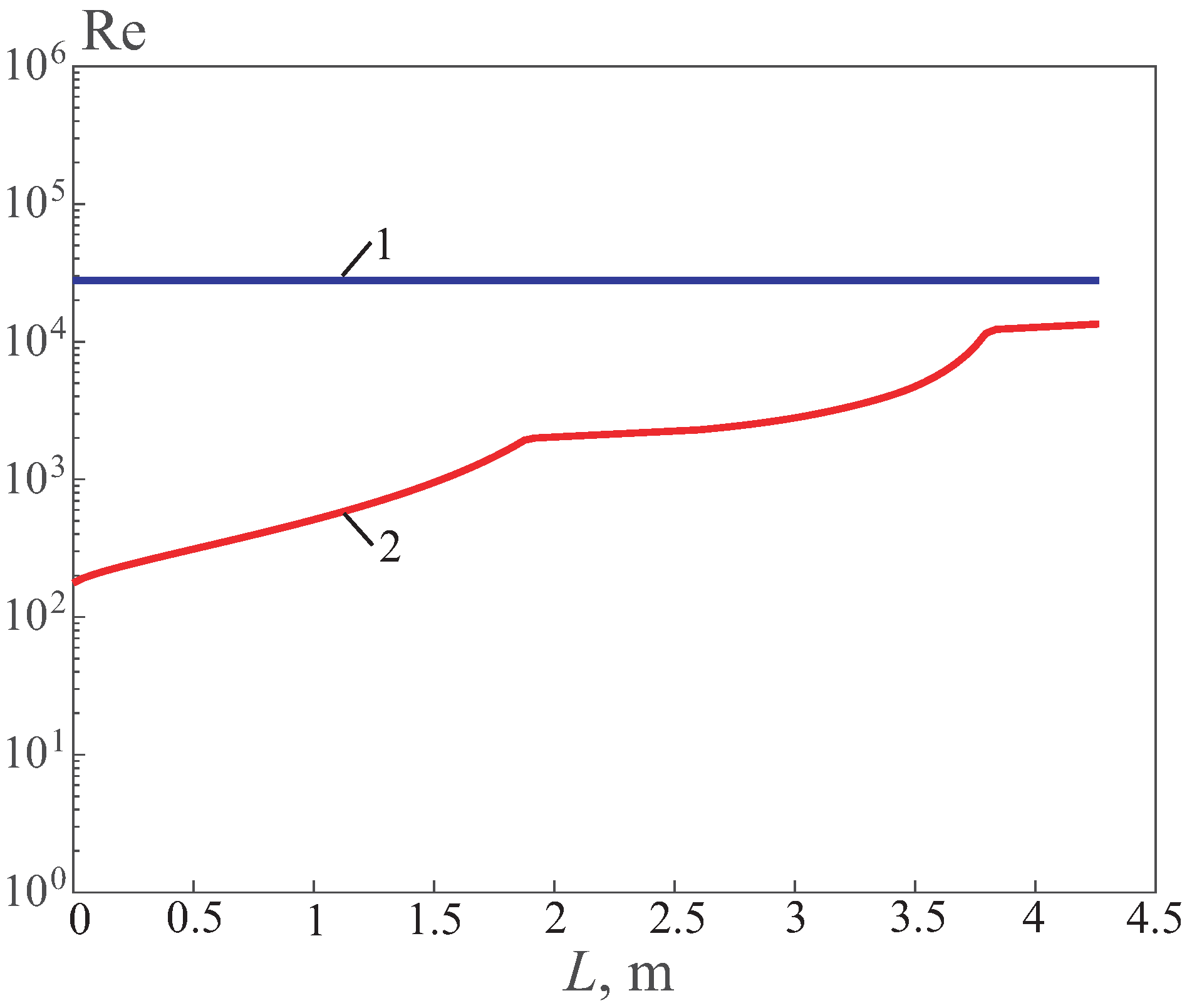
Figure 8 shows graphs of the change in the Reynolds number of coolants along the length, obtained in the calculation based on the model with the variable viscosity. For water, the Reynolds number practically does not change along the length at a constant value of viscosity and a slight change in the water temperature. The reverse picture is observed for a cold coolant (oil). The Reynolds number increases significantly along the length, which is associated with a sharp decrease in the viscosity of oil at its practically unchanged density. The figure also shows a transitional section at a distance from about 1.85 to 3.8 m, where the transition from the laminar to turbulent flow occurs.
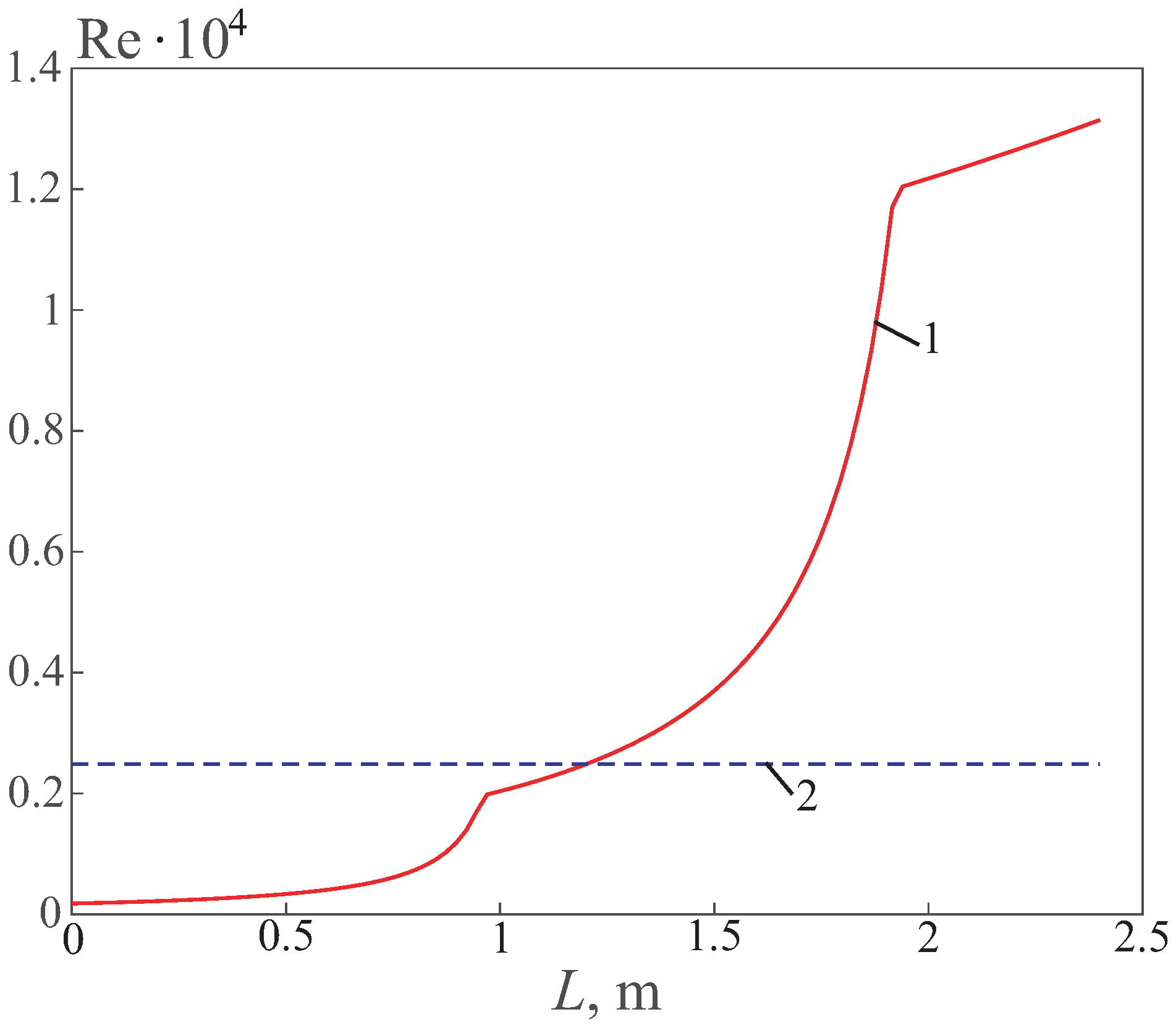
Figure 9 shows a graph of the change in the Reynolds number of oil (cold coolant) along the length of the heat exchanger at variable oil viscosity (line 1). The values of the Reynolds number sharply increase along the longitudinal coordinate, which is explained by a decrease in the viscosity of oil due to its heating. The figure also shows a graph of the behaviour of the Reynolds number of oil at an average coolant temperature (line 2). At a constant viscosity, the Reynolds number of the cold coolant is also constant along the length and cannot adequately characterize the heat transfer in a given heat exchanger. The first break corresponds to switching formulas at Re ∼2 × 10
(transition from laminar to transitional flow), and the second break corresponds to switching formulas at Re ∼10
(transition from transitional flow regime to turbulent). The work uses three sections and three different sets of formulas (laminar, transitional, and turbulent).
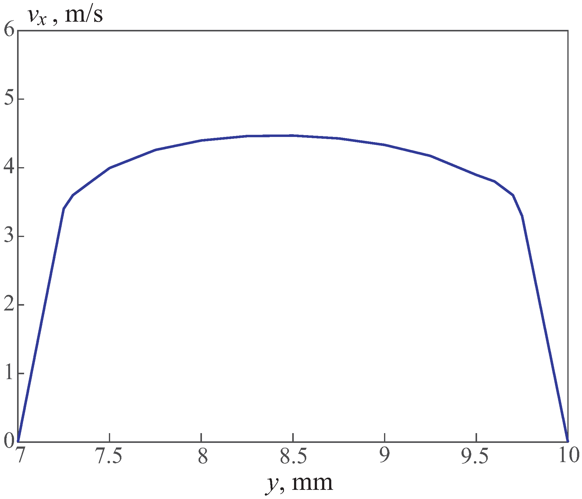
The distribution of the axial velocity of the coolant (oil) in various cross sections of the pipeline is shown in
Figure 10. In the cross section, the oil velocity varies from the maximum value on the axis of the pipeline to zero on its surface. The increase in the axial velocity at the outlet is explained by the decrease in the oil viscosity due to its heating as it approaches the outlet section. In this case, a turbulent flow regime occurs for oil.
Fluid enters the tube with a uniform velocity. When the fluid contacts the surface, viscous effects become important, and a boundary layer develops with an increasing axial coordinate. This development occurs at the expense of a shrinking inviscid flow region and concludes with the boundary layer merger at the centreline (hydrodynamic entry region). Following this merger, the viscous effects extend over the entire cross section, and the velocity profile no longer changes with the increasing axial coordinate (fully developed flow). The fully developed velocity profile is parabolic for the laminar flow in a circular tube. For the turbulent flow, the profile is flatter due to turbulent mixing in the radial direction. If a fluid enters the tube at a uniform temperature that is less than the surface temperature, convection heat transfer occurs, and a thermal boundary layer begins to develop. Moreover, if the tube surface condition is fixed by imposing either a uniform temperature or a uniform heat flux, a thermally fully developed condition is eventually reached. The shape of the fully developed temperature profile differs according to whether a uniform surface temperature or heat flux is maintained. For both surface conditions, however, the amount by which the fluid temperatures exceed the entrance temperature increases with the increasing axial coordinate.
The distribution of the axial velocity of water in the outlet section of the pipeline is shown in
Figure 11. The water velocity changes from zero on the wall to a maximum value on the channel axis. The flow of the water in this case is turbulent. The velocity profile has a character typical of the turbulent flow in a round pipe, being more filled near the axis and having large velocity gradients near the wall compared to the laminar flow.
The temperature distribution along the wall of the pipe through which the cold coolant flows is shown in
Figure 12. The temperature remains almost constant up to the cross section
m, after which a sharp increase in the temperature is observed. This behaviour is associated with the transition from the laminar flow regime to the turbulent one. At the inlet, the oil is cold and the wall on the oil side cools down strongly, then it warms up (heat transfer by thermal conductivity predominates), a laminar–turbulent transition occurs, the heat transfer increases significantly, and the wall temperature decreases.
On the graphs of the temperature distribution along the pipe, there is a steepening of the profile at the beginning of the transition zone (2.5–3 m), i.e., an increase in the heat exchange intensity. For example, if we consider a graph showing the distribution of the coefficient of friction along the length of the pipe, then, in the transition region, there is a dip in the coefficient of friction near the transition region.
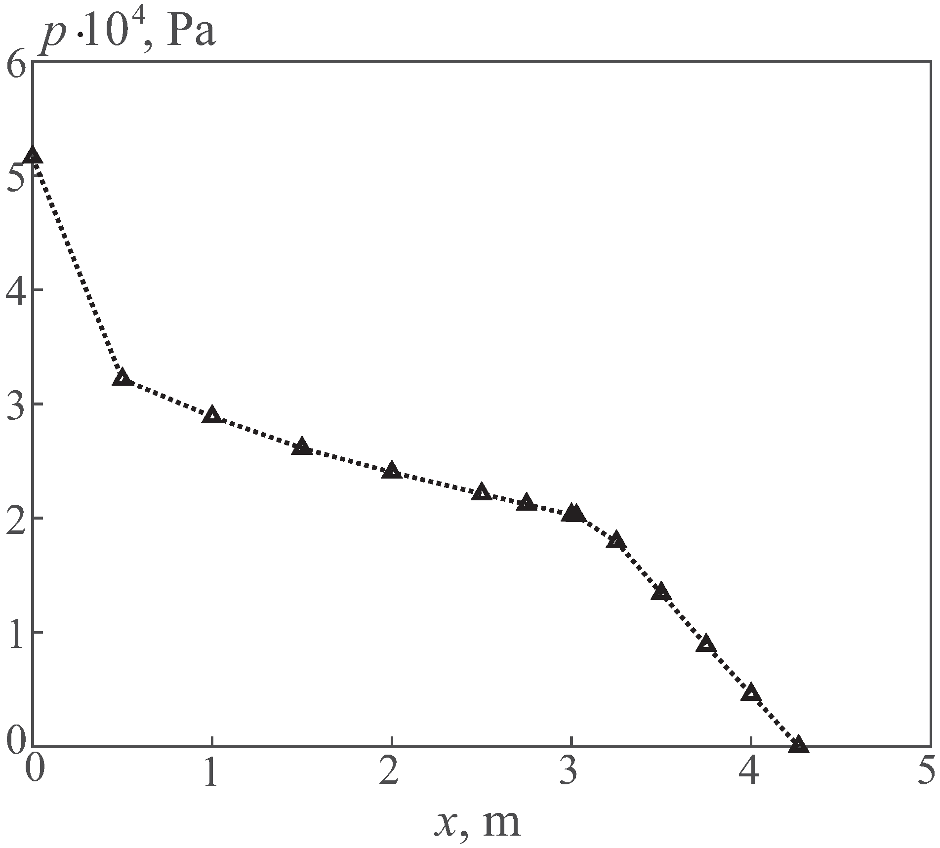
The distribution of the cross section-averaged oil pressure is shown in
Figure 13. In this case, the pressure drop along the entire length of the pipe is 51,613.89 Pa.
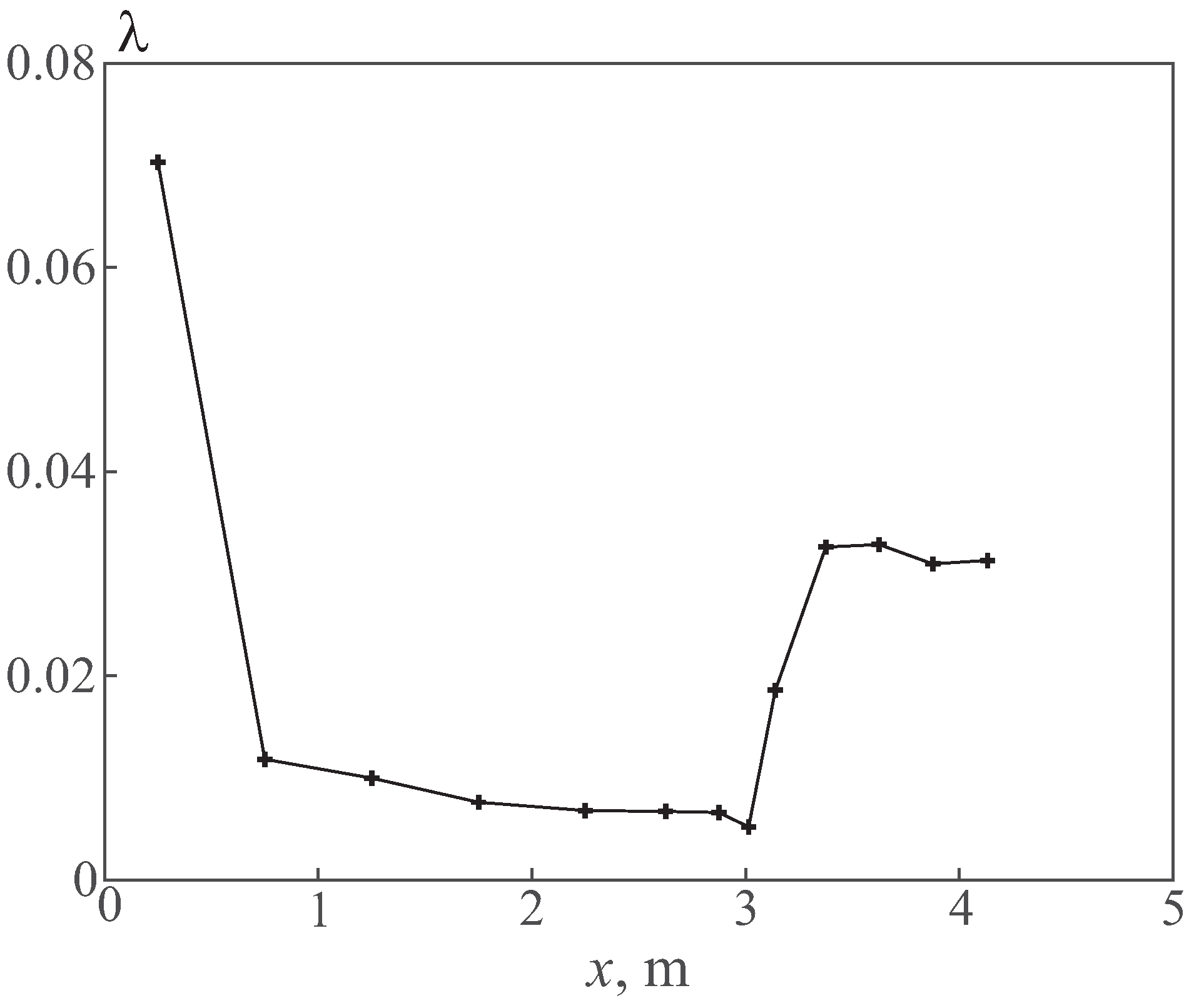
The change in the friction loss coefficient along the length of the pipe is shown in
Figure 14. The coefficient of the friction is calculated locally on a certain interval using the relation
, where
is the distance between two points, in which the pressure is measured, and
is pressure difference at these points.
7. Conclusions
Thermal and numerical calculations were carried out to determine the length of the heat exchanger and the temperature of the cold coolant in the outlet section in the case of constant and variable oil viscosity. The length of the heat exchanger was also determined using CFD calculations in a turbulence model that takes into account the laminar–turbulent transition. With a variable viscosity of oil, a transition from a laminar regime to a turbulent one is manifested, while, in the theoretical calculation method for a constant viscosity, this effect is not taken into account. The results obtained show that the model with constant viscosity leads to an underestimation of the length of the heat exchanger by about 20% compared to the calculations that take into account the dependence of the oil viscosity on temperature.


