

On the Determination of the 3D Velocity Field in Terms of Conserved Variables in a Compressible Ocean

Department of Meteorology, University of Reading, Reading RG6 6ET, UK
Fluids 2023, 8(3), 94; https://doi.org/10.3390/fluids8030094
Submission received: 31 December 2022
/
Revised: 3 March 2023
/
Accepted: 6 March 2023
/
Published: 8 March 2023
(This article belongs to the Collection Geophysical Fluid Dynamics)
Abstract
:Explicit expressions of the 3D velocity field in terms of the conserved quantities of ideal fluid thermocline theory, namely the Bernoulli function, density, and potential vorticity, are generalised in this paper to a compressible ocean with a realistic nonlinear equation of state. The most general such expression is the ‘inactive wind’ solution, an exact nonlinear solution of the inviscid compressible Navier–Stokes equation that satisfies the continuity equation as a consequence of Ertel’s potential vorticity theorem. However, due to the non-uniqueness of the choice of the Bernoulli function, such expressions are not unique and primarily differ in the magnitude of their vertical velocity component. Due to the thermobaric nonlinearity of the equation of state, the expression for the 3D velocity field of a compressible ocean is found to resemble its ideal fluid counterpart only if constructed using the available form of the Bernoulli function, the Bernoulli equivalent of Lorenz’s available potential energy (APE). APE theory also naturally defines a quasi-material, approximately neutral density variable known as the Lorenz reference density. This density variable, in turn, defines a potential vorticity variable that is minimally affected by thermobaric production, thus providing all the necessary tools for extending most results of ideal fluid thermocline theory to a compressible ocean.
1. Introduction
Although oceanic observations have increased dramatically in recent decades, especially since the development of the Argo floats program (https://argo.ucsd.edu, accessed on 7 March 2023), they still primarily constrain the density stratification rather than the velocity field. As a result, even in the most sophisticated ocean state estimate products [1,2,3,4], the realism of the simulated 3D oceanic velocity field can rarely, if ever, be ascertained directly. Indeed, even when current meters are available, they usually contain high-frequency motions linked to tides and gravity waves that are not usually captured by numerical ocean models, thus complicating the comparison. In any case, comparisons, when possible, are only limited to the horizontal velocity field as the vertical velocity is generally too small to be directly measurable.
Since, for all practical purposes, the 3D oceanic velocity field is not a measurable parameter of the system, the development of accurate dynamical theories that predict how to infer it from available oceanic observations plays an especially important role in physical oceanography. It is, therefore, no surprise that the subject has a long history going back to the early days of the discipline, which, to date, has primarily relied on the use of the dynamic method [5]. As is well known, the dynamic method assumes geostrophic and hydrostatic balances and provides an explicit expression of the horizontal velocity field in terms of the vertical integrals of the horizontal density gradients relative to the velocity field at some reference level. Understanding how to specify the latter is one of the main challenges of the dynamic method and has given rise to many different approaches to tackle it. The simplest approach, which is most often encountered in the literature, assumes the existence of a level of no motion at which the geostrophic velocity vanishes (see [6] for a discussion of its limitations). That approach has since been superseded by the beta-spiral method of [7] or the inverse method(s) of [8,9], whose connection is discussed in [10]. Refs. [11,12,13,14] are examples of studies that further discuss these ideas. At some point, there was hope that the sea surface height (SSH) signal measured by satellite altimetry would be accurate enough to constrain the surface geostrophic velocity field. However, this requires a more accurate determination of the geoid than is presently available. Moreover, the fact that the SSH signal is contaminated by small-scale and high-frequency processes while also reflecting transient variations of the interior density field complicates filtering out only the relevant part needed by the dynamic method [15]. More recently, measurements of Argo float displacements have shown promise for constraining the geostrophic velocity at the floats’ parking depth, as recently demonstrated in [16,17]. Nevertheless, some limitations remain, as Argo float displacements are also a priori impacted by energetic small-scale and transient ageostrophic motions in addition to the geostrophic flow, which the authors sought to mitigate by averaging over the Argo period. Outside the Argo period, or when focusing on time snapshots, alternative/complementary approaches for constraining the unknown reference level are still needed.
Although the geostrophic approximation is generally accepted to represent an accurate theory for the horizontal velocity field , how best to predict the vertical velocity field w is, in contrast, much less understood and still actively debated. Physically, there are two main fundamental approaches to thinking about the vertical velocity field. The first approach, which, as far as we are aware, underlies the computation of the vertical velocity field in all existing numerical ocean models [18], is based on vertically integrating the continuity equation . Doing so yields an expression for w controlled by the horizontal velocity divergence relative to the vertical velocity at some reference level
where is the horizontal nabla operator. As is well known, using the continuity equation in conjunction with geostrophy yields the celebrated linear Sverdrup balance , which may be integrated to yield
(see [19]), where f is the Coriolis parameter and , with y denoting the latitude. The second approach is based on extracting w from the conservation equation of any conserved tracer C, viz.,
where represents the non-material sinks/sources of C. Both approaches come with important theoretical challenges. In the first approach, the difficulty stems from the fact that the horizontal divergence is often dominated by the ageostrophic component of the velocity, in which case (2) may become very inaccurate. In the second approach, the difficulty is that the time derivative , and perhaps, to a lesser extent, the diabatic term , may both be important for predicting the large-scale vertical velocity field, yet are often hard (if at all possible) to constrain observationally. Existing approaches, therefore, can be regarded as attempts to mitigate these difficulties in some way. For instance, the well-known omega equation is obtained by artfully combining two prognostic equations (for vorticity and buoyancy, respectively) in a way that eliminates the time-derivative in each equation to formulate a diagnostic elliptic problem for the vertical velocity (see [20] for a recent implementation). Another approach of interest that shows how to infer the vertical velocity from individual moorings is that proposed in [21].
Physically, one key reason that makes the second approach potentially the most attractive is that if one ignores the difficulties associated with the time-dependent and diabatic terms and in (3), knowledge of the geostrophic velocity field is generally sufficient enough to accurately estimate the horizontal advection term . In contrast, knowledge of the ageostrophic velocity component is often needed for an accurate determination of the horizontal velocity divergence in the first approach, as mentioned above. As a result, there has been much interest in seeking to exploit the existence of quasi-material, conserved quantities to construct explicit expressions of the steady-state 3D velocity field. Thus, if and represent two independent conserved quantities, it is well known that in a steady state, the 3D velocity should lie at the intersection of two iso-surfaces of and . Mathematically, this implies that the velocity field can be written in the form
for some scalar field . Physically, the constraint determining is that the horizontal component of (4) be either exactly or approximately geostrophic. The conserved quantities and then determine the vertical velocity according to or or both, where and are the horizontal ‘slope’ vectors
Thus, depending on the conserved quantities considered, the relations and may or may not define the same vertical velocity. In practice, this means that the problem to be solved might be over-determined, and its resolution may require the use of least-squares methods.
Although (4) can, in principle, be implemented in practice using a variety of conserved tracers, three particular quantities deserve special attention owing to their theoretical and dynamical importance in oceanography, namely the Bernoulli function B, potential vorticity Q, and density . Physically, this is because these quantities are the ones that underlie the ideal fluid thermocline equations [22] that have formed the basis for most ocean circulation theories, as well as those originally considered by Needler [23], who pioneered the use of (4). Unfortunately, such quantities have, so far, been unambiguously defined only for an ideal fluid, which significantly hinders our ability to evaluate the usefulness of (4) for the real compressible ocean. Although several studies have since extended Needler’s approach, e.g., [24,25,26,27], most discussions with a few exceptions, e.g., [28,29], have remained limited to the case of an ideal fluid in geostrophic balance. To make progress, this paper aims to generalise Needler’s approach to the case of a fully compressible ocean in order to systematically test its usefulness in the future (which is beyond the scope of this paper). Section 2 reviews the basic properties of the ideal fluid thermocline equations and introduces the concept of the ‘available’ Bernoulli function. Section 3 shows how to generalise ideal fluid thermocline theory to compressible seawater and shows that the results are related to [30]’s ‘inactive wind’ solution. Section 4 discusses the results and some perspectives.
2. Absolute Velocity Field Based On Ideal Fluid Thermocline Theory
2.1. Thermodynamic Form of Ideal Fluid Thermocline Equations
We begin by briefly reviewing the properties and structure of the ideal fluid thermocline equations [22] that underlie Needler’s determination of the absolute velocity field in terms of conserved properties [23]. Although most of the material is standard, an important new element is the introduction of the concept of the ‘available’ Bernoulli function, where the term ‘available’ is meant to parallel that of Lorenz’s ‘available potential energy’ [31]. The ideal fluid thermocline equations are written in the following form
and describe the geostrophic and hydrostatic momentum balances, continuity, and conservation of density, respectively, where p is the pressure, is the density, g is the acceleration of gravity, and is the unit vector pointing upward. Although the geostrophic and hydrostatic balances are expected to meaningfully describe the balanced part of the flow even under transient evolution for a sufficiently small Rossby number, the steady form of the density equation in (8) is, in contrast, much more difficult to justify rigorously, especially without a clarification of what the density variable is supposed to represent. Presumably, any justification of (8) must consider some form of temporal averaging that does not introduce eddy-correlation terms, such as thickness-weighted averaging [32]. As the issue is quite complex and cannot fully be addressed without having first clarified the exact nature of , its full treatment is deferred to a subsequent study.
2.2. Available and Background Bernoulli Functions
One of the main ideas of this paper is that Lorenz’s APE theory holds the key to understanding how to generalise the key ingredients of ideal fluid thermocline theory, that is, the Bernoulli function, potential vorticity, and density, to a compressible ocean. The key ingredients needed here are the reference pressure and density profiles, denoted by and , respectively. These profiles characterise the Lorenz reference state of minimum potential energy that can be obtained through an adiabatic and isohaline re-arrangement of mass. Additionally, we require the reference position of a fluid parcel, , which is defined as the solution of the level of neutral buoyancy (LNB) equation . This definition yields as a function of density only [35,36,37]. Physically, the APE theory is useful for distinguishing between the potential energy that can be converted into kinetic energy in a reversible way (the APE) and the dynamically inert part of potential energy (the BPE) that cannot. Because the Bernoulli function is thermodynamic in nature, the same idea that only a fraction of it is available for reversible conversions with kinetic energy must apply. This motivates us to define its dynamically inert part in a Lagrangian sense as its value in a Lorenz reference state, viz.,
and the ‘available’ part of the Bernoulli function as
using the fact that, by definition, and , where the underbraced quantity can be recognised as the positive definite APE density that was originally introduced in [38,39] and later extended to multi-component Boussinesq and stratified fluids in [35,37]. Physically, the APE density can be written as the work against buoyancy forces needed to bring a fluid parcel from its level of neutral buoyancy (hence, satisfying to its actual position, viz.,
and the only difference between the expressions for a Boussinesq and a general compressible fluid is in the expressions for the buoyancy b. For a Boussinesq fluid, , whereas for compressible seawater, which is discussed in the next section, . Note that since , may also be rewritten as
so that for a small departure from the reference position,
which a reader unfamiliar with APE may still recognise. It also makes the positive definite character of clearer if needed.
Removing from both sides of (9) using the easily verified result that , yields the following available thermodynamic form of momentum balance
A key point to note here is that in both (9) and (15), the two P-vectors and are parallel to the gradient of density , and, therefore, perpendicular to the isopycnal surfaces . We see in Section 3 that this property is lost in a compressible ocean. It is of interest to note that is the ideal fluid counterpart of the P-vector previously identified in [40].
2.3. Bernoulli and Potential Vorticity (PV) Theorems
The Bernoulli theorem [41] and Ertel’s PV conservation theorem [42,43] play key roles in this paper. The former is trivially obtained by taking the inner product of (9) and (15) with , accounting for (8), which immediately yields and . The proof of the potential vorticity (PV) conservation theorem is somewhat more involved. To obtain it, first, divide (6) by and take the curl, thus leading to
Next, take the inner product of (16) with , which then yields
which establishes the material conservation of the potential vorticity (PV) as expected.
2.4. Determination of the Absolute Velocity Field in Terms of Conserved Quantities
Taking the cross product of with (9) or (15) and using the result that (which follows from the vector algebra relation and conservation of density , with being shorthand for ) leads, after some manipulation, to the following explicit expression of that was previously obtained in [23],
which explicitly relies on density and the Bernoulli function being conserved following fluid parcels, regardless of which form of the Bernoulli function is used (B refers indifferently to or ).
To show that (18) naturally satisfies the continuity equation as a consequence of Ertel’s PV conservation theorem, simply take its divergence, which yields
QED. As a result, (18) represents an exact steady solution of the ideal fluid Equations (6)–(8) that, in addition to the horizontal velocity, predicts the vertical velocity
Importantly, Needler’s formula (22) is insensitive to the particular choice of Bernoulli function—B or —used to estimate it due to being a function of only.
2.5. Bernoulli Method
Physically, one key reason that Needler’s formula (18) is appealing is that the idea that the steady or time-averaged 3D velocity field should lie at the intersection of the iso-surfaces of two conserved quantities is a priori valid beyond the geostrophic approximation. Its other key advantage is that it naturally satisfies the continuity equation as a consequence of Ertel’s potential vorticity conservation theorem, which also generalises beyond the geostrophic approximation, as discussed in the next section. In the context of the dynamic method, however, Needler’s formula does not, in itself, solve the problem of the unknown reference level. Indeed, because , it is easily verified that the horizontal velocity it predicts is the standard geostrophic balance, whereas the vertical velocity predicted in (20) is predicted more easily from the density equation , i.e.,
where is the slope vector associated with the isopycnal surfaces. In other words, Needler’s formula does not solve the problem of the unknown reference level because the Bernoulli function depends on the same unknown constant of integration as the pressure field.
To circumvent the difficulty and make (18) useful, it is necessary to invoke the result that if , B, and Q are all conserved along fluid parcel trajectories, they must be functionally related. Thus, to the extent that such a result holds and this functional relationship may be written in the form , it is possible to rewrite (18) as
[23]. Now, the key advantage of (22) over (18) is that the term can, in principle, be empirically estimated from climatological fields without having to solve the problem of the unknown reference level since the latter affects neither nor Q. In other words, (22) provides a determination of the absolute velocity field up to the multiplicative constant . In this approach, the problem of the unknown reference level, therefore, transforms into the problem of how best to evaluate the functional relationship and the partial derivative . For related discussions of these ideas, the reader is referred to, e.g., [13,24,25,26,27,28,44,45]. However, it seems fair to say that the current empirical evidence for a well-defined relationship is inconclusive at best. Current approaches, however, have relied on using the conventional form of the Bernoulli function rather than its available form . It will be of interest in future studies to test whether using , as well as the density variable discussed in the next section, can lead to a better-defined relationship .
3. Generalisation to Compressible Seawater
3.1. Governing Equations for Compressible Seawater
We now turn to a realistic nonlinear ocean described by the compressible Navier–Stokes equations, treating seawater as a two-constituent stratified fluid:
where is the specific entropy, S is the salinity, is the specific volume, is a friction force, and is the geopotential. Moreover, and denote the diabatic sources/sinks of heat and salt due to molecular diffusive fluxes (radiation can be included if needed). As in the previous section, the first step is to rewrite the momentum balance (23) in its thermodynamic or Crocco–Vazsonyi form
where is the absolute vorticity and is the relative vorticity. The results were obtained using the well-known relation , as well as the total differential for the specific enthalpy , where T is the in situ temperature and is the relative chemical potential. For a compressible ocean, the conventional form of the Bernoulli function is
whereas the P-vector is the vector that retains the thermohaline gradient of h, viz.,
As in the previous section, we introduce the available Bernoulli function as , that is, as the difference between the conventional form of the Bernoulli function and the background Bernoulli function
where, as before, is the reference height of a fluid parcel in Lorenz’s reference state of minimum potential energy, which, in practice, may be computed using the computationally efficient algorithm of Saenz et al. [36]. Physically, is defined as before as a solution of the level of neutral buoyancy equation, which, for two-component compressible seawater, takes the form
where . The available Bernoulli function may thus be written in the form
where is the potential energy density defined in [37], and and are the subcomponents
As explained and demonstrated in [37], both and are positive definite. may be interpreted as the available compressible energy (ACE), which represents the expansion/contraction work required to compress/expand from the reference pressure to the actual pressure. As for , it is the APE density and represents the work against the buoyancy forces required to move the fluid parcel from its reference position at pressure to its actual position z at pressure . As before, the available thermodynamic form of the momentum balance is obtained by removing from both sides of (27), which leads to
where the P-vector takes the form
Note that the suffix ‘r’ denotes the thermodynamic quantities estimated at the reference pressure .
3.2. Comparison of Ideal and Compressible Forms of Bernoulli Functions and P-Vectors
In an ideal fluid, Needler’s formula (18) defines the 3D velocity field as being perpendicular to the density surfaces , regardless of the particular form of used due to and both being parallel to in that case. The 3D velocity field is also perpendicular to the iso-surfaces of the Bernoulli function in both cases but, generally, the iso-surfaces of and should appear distinct from each other. Whether the available form is superior to the conventional form cannot be determined from theoretical considerations alone; however, it is possible that the assumed empirical functional relationship underlying the Bernoulli method may be more accurately achieved in climatological observations of the density field by using one of the forms of .
The situation is different for compressible seawater, however, as and now, generally, define different directions, as is clear from Equations (29) and (36). Moreover, it is easily verified that both P-vectors have a non-zero helicity because of thermobaricity and are, therefore, both non-integrable. Mathematically, this means that it is not possible to identify a well-defined seawater variable whose iso-surfaces are everywhere perpendicular to . From a theoretical perspective, this is both interesting and important, as it suggests that the superior form of may be the one for which the compressible and ideal expressions resemble each other the most.
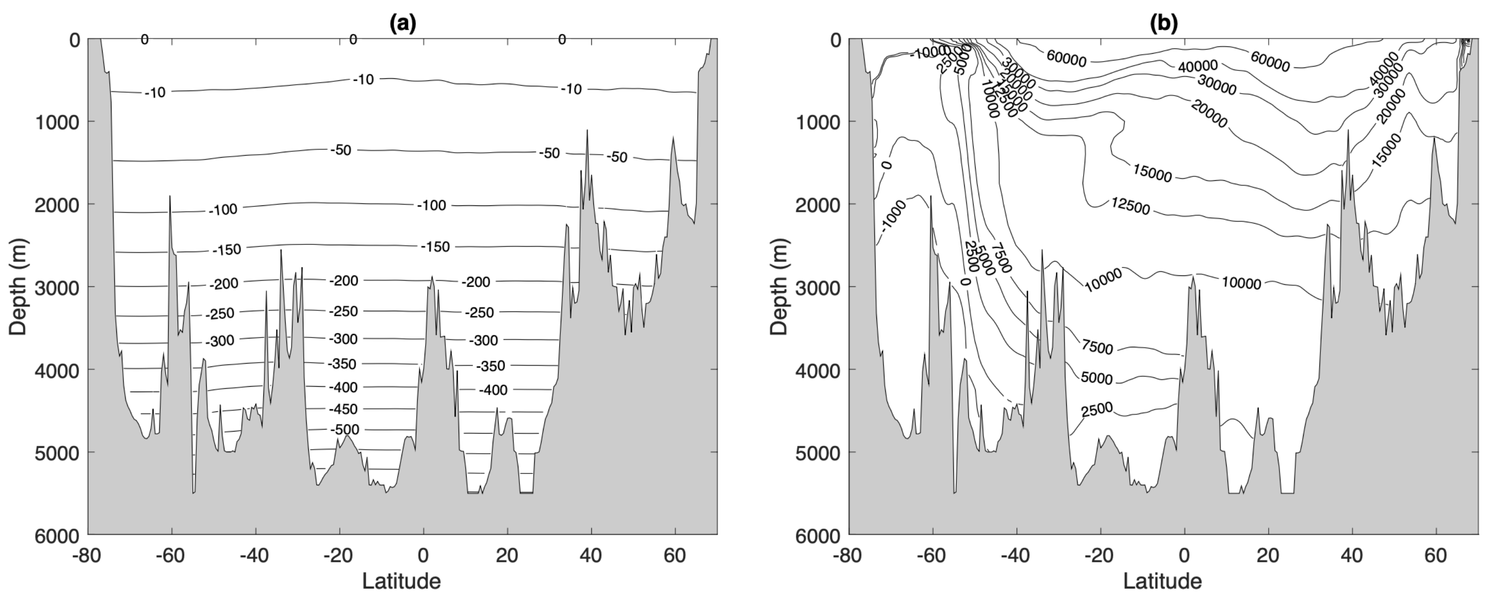
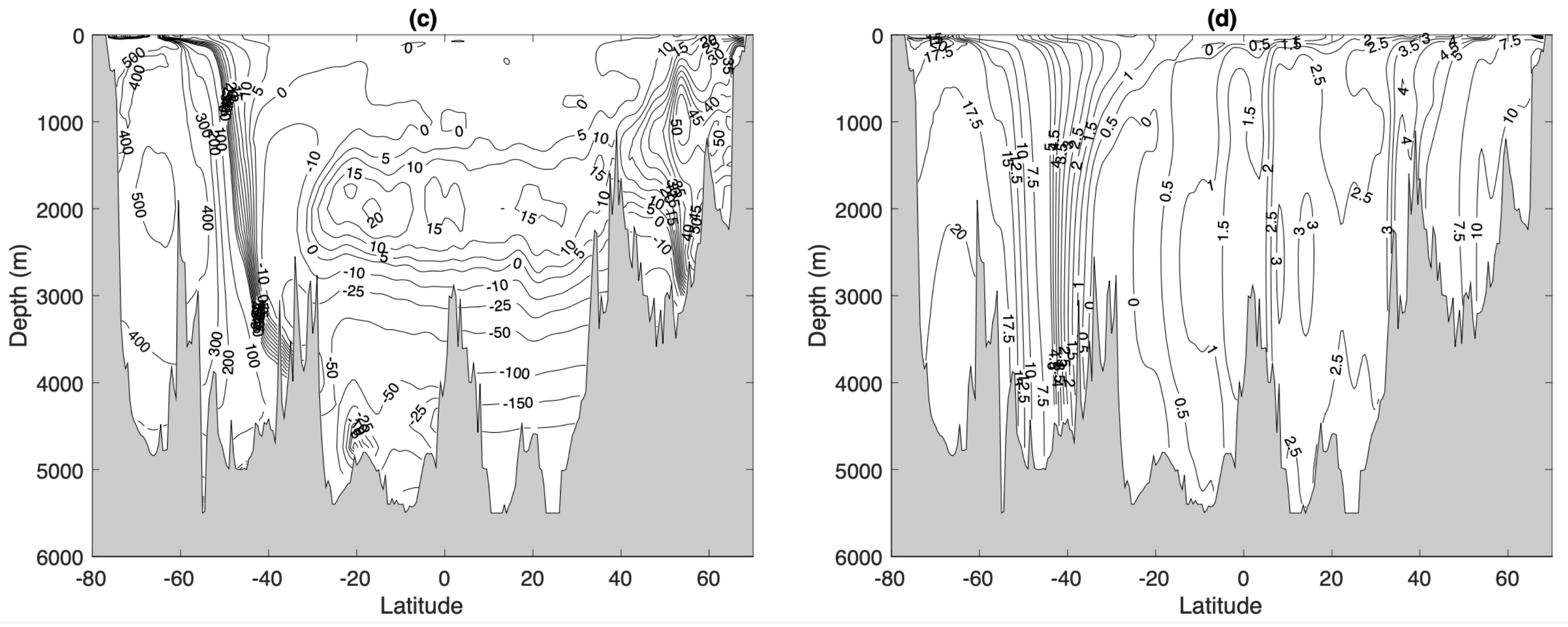
To explore this idea, Table 1 summarises the forms of the Bernoulli function and P-vectors for the ideal and compressible forms established in the previous sections, whereas Figure 1 illustrates the four different types of Bernoulli functions along the W meridional section in the Atlantic Ocean. We used the WOCE climatological dataset [46] and computed the hydrostatic pressure, assuming a level of no motion at 1500 . The Lorenz reference density and pressure profiles, as well as the reference depths, were computed as in [47]. The contribution from the kinetic energy was ignored. The figure clearly shows that the Bernoulli function depends sensitively on the approach considered, as well on the choice of the arbitrary constants entering the definition of the specific enthalpy, as defined by TEOS-10 (www.teos-10.org, accessed on 7 March 2023). In the figure, panel (a) shows that the ideal standard Bernoulli function is dominated by its depth variations, with values increasing in height from −700 at depth to close to 0 at the surface. In contrast, the compressible standard Bernoulli function (panel (b)), which depends on the TEOS-10 definition of the specific enthalpy, is dominated by thermal variations near the surface that result in much bigger values overall, which also increase in height from about close to zero at depth to about 60,000 near the surface. The ideal and compressible forms of the available Bernoulli function are depicted in panels (c) and (d), respectively. Although our theory predicts that the latter should be close to each other, this is not the case in practice because our prediction in (11) assumes an incompressible , which is not true of in situ density. Panel (d) shows that the compressible available Bernoulli function is dominated by horizontal variations. This seems to be an optimal behaviour for plotting it on isopycnal surfaces, which will be discussed in detail in a subsequent study. Note that the values exhibited by , which range approximately from 0 to 20 , are considerably smaller than that of all other Bernoulli functions, confirming the idea that is the only one not affected by irrelevant dynamical information, which we hope can be exploited in the future.
3.2.1. Conventional Bernoulli Function
By contrasting the ideal and compressible forms of the conventional Bernoulli function,
it is clear that the two expressions are not easily related. The difference in behaviour between and can be further evidenced by contrasting, for instance, their vertical derivatives, leading to
In order to link to the vertical derivative of some density variable, one needs to make use of the Maxwell relations attached to the total differential of the enthalpy , which is obtained by stating the equality of the cross derivatives, viz.,
To proceed, let us now introduce a reference pressure that is envisioned as being not too different from p, defining the reference values and . If we also use use the approximation , (39) can be rewritten as
where is the potential density referenced to (or more accurately to ), where the result assumes that is close enough to p that the overbar value can be approximated by their values at . Although the first term of (41) succeeds in showing dependence on the vertical derivative of some density variable that makes it directly comparable to , the second term is extraneous. Using the same ideas, it is also easily established that the same difficulties exist in relating to .
3.2.2. Available Bernoulli Function
In contrast, it is immediately apparent that the ideal and compressible available Bernoulli functions
are directly comparable, as can be obtained from by neglecting and replacing with in , as Tailleux [37] showed that closely resembled . Likewise, it is possible to show that the APE-based P-vectors resemble each other
To see the connection, one may use the Maxwell relations (40) to establish that
using the fact that , , and , where , , etc. This shows that is intermediate between the locally-referenced gradients referenced to the local and reference pressure, respectively, which means that it is close to the standard neutral vector considered in [48]. In other words, is approximately parallel to the gradient of the potential density referenced to the mid pressure . For a more extensive discussion of this link, see [49].
The above considerations clearly establish that the results of ideal fluid thermocline theory can only be generalised to compressible seawater if the available form rather than the conventional form is used.
3.3. Inactive Wind Solutions
To discuss how to extend Needler’s formula to compressible seawater, we consider the steady and inviscid momentum equations written in their thermodynamic, or Crocco–Vazsonyi, form
(from Equations (27) and (35)), where the subscript indicates whether the conventional or available form of B and is used. To simplify the notations, this subscript is dropped in the following and re-introduced only when needed. For a small Rossby number, as pertains to the large-scale motions of interest here, the relative vorticity and kinetic energy only affect and B at second order. Equation (45) is then an under-determined linear system for that can only be solved if the following solvability condition is satisfied
(obtained by taking the inner product of (45) with ), so that in (45) is determined only up to an arbitrary vector parallel to , with a scalar field. The solution of (45) that is perpendicular to both and and is the counterpart of Needler’s formula (18), is easily verified to be
whereas the counterpart of is
which is the equality following from (46). In the context of a dry atmosphere, [30] derived an expression similar to (47) and referred to as the ‘inactive wind’.
In order to examine the consistency of the inactive wind solution (47) with mass conservation, let us take the divergence of , which yields
Similarly as for one of Needler’s formulas, is shown here to satisfy the continuity equation as a consequence of Ertel’s PV conservation theorem applied to the PV constructed from the Bernoulli function . To show this, let us recall that in its most general form, [50]’s theorem (see [43] for an English translation) establishes that for any scalar , the PV variable can be shown to satisfy the conservation law
(e.g., see Equation 4.95 in [51]). To make the link with (49), it is important to understand the different equivalent forms that the baroclinic production term (the term proportional to in (50)) may assume. As seen previously, from the definitions of and , we have the following equivalence relations
Taking the curl yields the following equivalent expressions
which are proportional to the baroclinic production term, where is the so-called N-neutral vector entering [48]’s definition of (approximately) neutral surfaces (ANS). Now, if we use in the inviscid case and invoke the Bernoulli theorem, , (50) predicts that
Comparing this with (49) shows that
as expected, thus confirming that satisfies the continuity equation regardless of which form of is used.
3.4. Uniqueness of the Inactive Wind Solution
The two inactive wind solutions introduced above may be written explicitly as
Since these two solutions both satisfy the continuity equation, a question that naturally arises is whether they define the same velocity field despite being constructed from different fields. To examine this, let us recall that, by definition, , whereas . It follows that
which suggests that and define two different vector fields. However, because they both represent an exact solution of (45), it follows that their difference must be proportional to the null-space solution . In other words, there must exist some scalar such that
For a small Rossby number, (where f is the Coriolis parameter), which implies that and must primarily differ by their vertical velocity component. Physically, this is plausible because in this case, the horizontal components of and must both be approximately geostrophic, i.e., , whereas their vertical components must satisfy and , respectively, where and are the horizontal slope vectors defined by and , respectively. As a result,
which confirms that the two vertical velocities and might differ if the slopes defined by the two different P-vectors differ, as is generally the case. It is of interest to ascertain whether the vertical velocity component of is a better predictor of the actual vertical velocity field than that of , which we plan on investigating in a subsequent study.
3.5. Reformulation in Terms of Quantities Independent of Pressure
Let denote an approximately neutral quasi-material density variable and denote the PV variable constructed from it. As discussed in [36,47,49,52], APE theory naturally includes a generalised form of the potential density that is naturally very accurately neutral outside the Southern Ocean (even more so than Jackett and McDougall [53]’s empirical neutral density variable while also being mathematically and physically well defined. This motivated [47,52] to define thermodynamic neutral density as
where is a polynomial pressure correction empirically fitted to make look as much like . Because it tends to be more accurately neutral than outside the Southern Ocean, is the variable that is currently the least affected by the thermobaric production term.
If one accepts and as the most sensible generalisations of the concepts of density and PV to compressible seawater, then one may proceed similarly to [23] and assume that if B, , and are all approximately conserved along fluid parcel trajectories, a functional relationship should exist between B, , and , say , as in ideal fluid thermocline theory. Then, the seawater counterpart of Needler’s second formula (22) becomes
In comparison to Needler’s formula, (60) possesses the extra and undesirable thermobaricity-induced term proportional to . This term can only be neglected if rather than is used, as the angle between and is not generally small enough. If so,
which is more directly comparable to (22), stressing again the fundamental importance of APE theory to extend the results of ideal fluid thermocline theory to compressible seawater.
4. Discussion
The idea that steady fluid parcel trajectories lie at the intersection of the iso-surfaces of conserved quantities is arguably one of the most promising avenues of research for progressing the theory of the 3D oceanic velocity field. This is because this idea is a priori as equally valid for an ideal fluid for which it was originally developed by [23] as it is for a fully compressible ocean with a realistic nonlinear equation of state, as recently initiated by [29]. In this paper, we made significant progress towards generalising this idea to compressible seawater, encapsulated into three main new results.
Our first main result is that Needler’s formula (18) can be interpreted as a linear approximation of a much more general nonlinear and exact solution of the compressible NSE called the ’inactive wind’ solution. This solution was previously derived by [30] in the context of a dry atmosphere and was extended here to two-component compressible seawater. Like Needler’s formula, the inactive wind solution satisfies the continuity equation as a consequence of Ertel’s PV conservation theorem [42] (that is itself related to the generalised Bernoulli theorem of [41]). Like Needler’s formula, the inactive wind solution is perpendicular to the gradient of the Bernoulli function but unlike Needler’s formula, it is perpendicular to a vector rather than to the gradient of density . Physically, the inactive wind solution is most easily obtained by rewriting the momentum equations in their Crocco–Vazsonyi, or thermodynamic, form, which appears to be the most illuminating form for relating the 3D velocity field to the conserved quantities of the fluid.
Our second main result is that both Needler’s formula and the inactive wind solution are sensitive to how the Bernoulli function is defined, as it is always possible to redefine the latter by subtracting an arbitrary quasi-material function of (for a simple fluid) or S and (for compressible seawater). We find that only if the ‘available’ form of the Bernoulli function is used is it possible to meaningfully relate the inactive wind solution to Needler’s formula. Physically, the available Bernoulli function is defined as the difference between the conventional Bernoulli function and its background reference value in Lorenz’s state of minimum potential energy entering Lorenz’s APE theory [31]. Indeed, only in this case is the vector parallel to an approximately neutral density variable, namely the Lorenz reference density (LRD), which is discussed at length in [47,49,52].
Our third main result is that inactive wind solutions defined for different forms of the Bernoulli function and vector do not necessarily define the same 3D velocity field, even if each represents an exact solution of the compressible NSE satisfying the continuity equation. Mathematically, this is because the nonlinear balance equation from which the inactive wind solution is determined is degenerate. For a small Rossby number, this is equivalent to saying that different inactive wind solutions differ primarily in their vertical velocity components. More generally, this result means that although in principle, it is possible to construct a 3D velocity field as in terms of any arbitrary conserved quantities and for some , this does not necessarily imply that all constructions define the same velocity field, which does not appear to have received much attention so far. Physically, this is important because it provides the means, at least in principle, to test the usefulness of different constructions by comparing the 3D velocity field that each expression predicts with the 3D velocity field from any dynamically consistent ocean state estimate, as we plan on pursuing in a subsequent study.
The present results are important because we believe that they can pave the way for a more rigorous and general theory of the oceanic 3D velocity field valid for a realistic compressible ocean, as we hope to further demonstrate through concrete applications in future studies.
Funding
This research has been supported by the NERC-funded OUTCROP project (grant no. NE/R010536/1).
Data Availability Statement
The WOCE Global Ocean Climatology 1990–1998 (file ‘wghc_params.nc’) used in this study is available at https://doi.org/10.25592/uhhfdm.8987, accessed on 7 March 2023. Enthalpy and other functions of state were estimated using the TEOS-10 library available at www.teos-10.org, accessed on 7 March 2023. Software to compute the analytic form of thermodynamic neutral density is available at https://doi.org/10.5281/zenodo.4957697, accessed on 7 March 2023. See also the author’s website https://github.com/GammaTN for regular software updates and illustrative code examples.
Acknowledgments
The author gratefully acknowledges comments from A. Colin de Verdière and Geoff Stanley on a original version of the paper, as well as constructive and supportive comments from three anonymous referees.
Conflicts of Interest
The author declares no conflict of interest.
Abbreviations
The following abbreviations are used in this manuscript:
| PV | Potential Vorticity |
| APE | Available Potential Energy |
| ACE | Available Compressible Energy |
| LRD | Lorenz Reference Density |
| ANS | Approximately Neutral Surface |
| NSE | Navier–Stokes Equations |
References
- Lee, T.; Awaji, T.; Balmaseda, M.A.; Greiner, E.; Stammer, D. Ocean State Estimation for Climate Research. Oceanography 2009, 22, 160–167. [Google Scholar] [CrossRef]
- Forget, G.; Ferrerira, D.; Liang, X. On the observability of turbulent transport rates by ARGO: Supporting evidence from an inversion experiment. Ocean. Sci. 2015, 11, 839–853. [Google Scholar] [CrossRef] [Green Version]
- Masuda, S.; Osafune, S. Ocean state estimations for synthesis of ocean-mixing observations. J. Oceanogr. 2021, 77, 359–366. [Google Scholar] [CrossRef]
- Wunsch, C.; Ferrari, R. 100 years of the ocean general circulation. A century of progress in atmospheric and related sicences: Celebrating the american meteorological society centennial. Meteorol. Monogr. 2018, 59, 1–32. [Google Scholar] [CrossRef]
- Fomin, L.M. The Dynamic Method in Oceanography; Elsevier Oceanography Series 2; Elsevier: Amsterdam, The Netherlands, 1964. [Google Scholar]
- Olbers, D.J.; Willebrand, J. The level of no motion in an ideal fluid. J. Phys. Oceanogr. 1984, 14, 203–212. [Google Scholar] [CrossRef]
- Schott, F.; Stommel, H. Beta spirals and absolute velocities in different oceans. Deep-Sea Res. 1978, 16, 301–323. [Google Scholar] [CrossRef]
- Wunsch, C. Determining the general circulation of the oceans: A preliminary discussion. Science 1977, 196, 871–875. [Google Scholar] [CrossRef] [PubMed]
- Wunsch, C. The North Atlantic general circulation west of 50W determined by inverse methods. Rev. Geophys. 1978, 16, 583–620. [Google Scholar] [CrossRef]
- Davis, R.E. On estimating velocity from hydrographic data. J. Geophys. Res. 1978, 83, 5507–5509. [Google Scholar] [CrossRef]
- Behringer, D.W. On computing the absolute geostrophic velocity spiral. J. Mar. Res. 1979, 37, 459–470. [Google Scholar]
- Behringer, D.W.; Stommel, H. The beta spiral in the North Atlantic subtropical gyre. Deep-Sea Res. 1980, 27A, 225–238. [Google Scholar] [CrossRef]
- Killworth, P.D. A Bernoulli inverse method for determining the ocean circulation. J. Phys. Oceanogr. 1986, 16, 2031–2051. [Google Scholar] [CrossRef]
- Bigg, G.R. The beta spiral method. Deep Sea Res. 1985, 32, 465–484. [Google Scholar] [CrossRef]
- Park, Y.H. Determination of the surface geostrophic velocity field from satellite altimetry. J. Geophys. Res. Ocean. 2004, 109. [Google Scholar] [CrossRef] [Green Version]
- Colin de Verdière, A.; Ollitrault, M. A direct determination of the world ocean barotropic circulation. J. Phys. Oceanogr. 2016, 46, 255–273. [Google Scholar] [CrossRef] [Green Version]
- Colin de Verdière, A.; Meunier, T.; Ollitrault, M. Meridional overturning and heat transport from Argo floats displacements and the planetary geostrophic method (PGM): Application to the subpolar North Atlantic. J. Geophys. Res. Oceans 2019, 124, 5309–6432. [Google Scholar] [CrossRef] [Green Version]
- Griffies, S.M. Fundamentals of Ocean Models; Princeton University Press: Princeton, NJ, USA, 2004; p. 424. [Google Scholar]
- Wunsch, C. The decadal mean ocean circulation and Sverdrup balance. J. Mar. Res. 2011, 69, 417–434. [Google Scholar] [CrossRef] [Green Version]
- Nardelli, B.B. A multi-year time series of observation-based 3D horizontal and vertical quasi-geostrophic global ocean currents. Earth Syst. Sci. Data 2020, 12, 1711–1723. [Google Scholar] [CrossRef]
- Sevellec, F.; Garabato, A.C.N.; Brearley, J.A.; Sheen, K.L. Vertical flow in the Southern Ocean estimated from individual moorings. J. Phys. Oceanogr. 2015, 45, 2209–2220. [Google Scholar] [CrossRef] [Green Version]
- Welander, P. The thermocline problem. Philos. Trans. R. Soc. Lond. A. 1971, 270, 415–421. [Google Scholar] [CrossRef]
- Needler, G.T. The absolute velocity as a function of conserved measurable quantities. Prog. Oceanogr. 1985, 14, 421–429. [Google Scholar] [CrossRef]
- Chu, P.C. P-vector method for determining absolute velocity from hydrographic data. Mar. Tech. Soc. J. 1995, 29, 3–14. [Google Scholar]
- Chu, P.C. P-vector spirals and determination of absolute velocities. J. Oceanogr. 2000, 56, 591–599. [Google Scholar] [CrossRef]
- Kurgansky, M.V.; Budillon, G.; Salusti, E. Tracers and potential vorticities in ocean dynamics. J. Phys. Oceanogr. 2002, 32, 3562–3577. [Google Scholar] [CrossRef]
- Kurgansky, M.V. On the determination of the absolute velocity of steady flows of a baroclinic fluid with applications to ocean currents. Dyn. Atms. Oceans 2021, 95, 101234. [Google Scholar] [CrossRef]
- McDougall, T.J. The influence of ocean mixing on the absolute velocity vector. J. Phys. Oceanogr. 1995, 25, 705–725. [Google Scholar] [CrossRef]
- Ochoa, J.; Badan, A.; Sheinbaum, J.; Castro, J. ‘Preferred trajectories’ defined by mass and potential vorticity conservation. Geofis. Int. 2020, 59-3, 195–207. [Google Scholar] [CrossRef]
- Gassmann, A. Deviations from a general nonlinear wind balance: Local and zonal-mean perspectives. Met. Zeit 2014, 23, 467–481. [Google Scholar] [CrossRef]
- Lorenz, E.N. Available potential energy and the maintenance of the general circulation. Tellus 1955, 7, 138–157. [Google Scholar] [CrossRef] [Green Version]
- Young, W.R. An exact thickness-weighted average formulation of the Boussinesq equations. J. Phys. Oceanogr. 2012, 42, 692–707. [Google Scholar] [CrossRef]
- Crocco, L. Eine neue Stromfunktion für die Erforschung der Bewegung der Gase mit Rotation. ZAMM Z. Angew. Math. Mech. 1937, 17, 1–7. [Google Scholar] [CrossRef]
- Vazsonyi, A. On rotational gas flows. Quart. Appl. Math. 1945, 3, 29–37. [Google Scholar] [CrossRef] [Green Version]
- Tailleux, R. Available potential energy density for a multicomponent Boussinesq fluid with a nonlinear equation of state. J. Fluid Mech. 2013, 735, 499–518. [Google Scholar] [CrossRef] [Green Version]
- Saenz, J.A.; Tailleux, R.; Butler, E.D.; Hughes, G.O.; Oliver, K.I.C. Estimating Lorenz’s reference state in an ocean with a nonlinear equation of state for seawater. J. Phys. Oceanogr. 2015, 45, 1242–1257. [Google Scholar] [CrossRef] [Green Version]
- Tailleux, R. Local available energetics of multicomponent compressible stratified fluids. J. Fluid Mech. 2018, 842. [Google Scholar] [CrossRef] [Green Version]
- Holliday, D.; McIntyre, M.E. On potential energy density in an incompressible, stratified fluid. J. Fluid Mech. 1981, 107, 221–225. [Google Scholar] [CrossRef]
- Andrews, D.G. A note on potential energy density in a stratified compressible fluid. J. Fluid Mech. 1981, 107, 227–236. [Google Scholar] [CrossRef]
- Nycander, J. Energy conversion, mixing energy, and neutral surfaces with a nonlinear equation of state. J. Phys. Oceanogr. 2011, 41, 28–41. [Google Scholar] [CrossRef]
- Schär, C. A generalization of Bernoulli’s theorem. J. Atm. Sci. 1993, 50, 1437–1443. [Google Scholar] [CrossRef]
- Muller, P. Ertel’s potential vorticty theorem in physical oceanography. Rev. Geophys. 1995, 33, 67–97. [Google Scholar] [CrossRef]
- Schubert, W.; Ruprecht, E.; Hertenstein, R.; Ferreira, R.N.; Taft, R.; Rozoff, C.; Ciesielski, P.; Kuo, H.C. English translations of twenty-one of Ertel’s papers on geophysical fluid dynamics. Meteo. Zeitschrift 2004, 13, 527–576. [Google Scholar] [CrossRef] [Green Version]
- Killworth, P.D. A note on velocity determination from hydrographic data. J. Geophys. Res. 1979, 84, 5093–5094. [Google Scholar] [CrossRef]
- Killworth, P.D. On determination of absolute velocities and density gradients in the ocean from a single hydrostatic section. Deep-Sea Res. 1980, 27A, 901–929. [Google Scholar] [CrossRef]
- Gouretski, V.V.; Koltermann, K.P. WOCE global hydrographic climatology. Berichte Bundesamtes Seeshifffahrt Hydrogr. Tech. Rep. 2004, 35, 49. [Google Scholar]
- Tailleux, R. Spiciness theory revisited, with new views on neutral density, orthogonality and passiveness. Ocean. Sci. 2021, 17, 203–219. [Google Scholar] [CrossRef]
- McDougall, T.J. Neutral surfaces. J. Phys. Oceanogr. 1987, 17, 1950–1964. [Google Scholar] [CrossRef]
- Tailleux, R.; Wolf, G. On the links between thermobaricity, available potential energy, neutral directions, buoyancy forces, potential vorticity, and lateral stirring in the Ocean. J. Phys. Oceanogr. 2023. submitted. [Google Scholar] [CrossRef]
- Ertel, H. Ein neuer hydrodynamisher Wirbelsatz. Meteo. Z. 1942, 59, 277–281. [Google Scholar]
- Vallis, G.K. Atmospheric and Oceanic Fluid Dynamics; Cambridge University Press: Cambridge, UK, 2006; p. 745. [Google Scholar]
- Tailleux, R. Generalized patched potential density and thermodynamic neutral density: Two new physically based quasi-neutral density variables for ocean water masses analyses and circulation studies. J. Phys. Oceanogr. 2016, 46, 3571–3584. [Google Scholar] [CrossRef]
- Jackett, D.R.; McDougall, T.J. A neutral density variable for the World’s oceans. J. Phys. Oceanogr. 1997, 27, 237–263. [Google Scholar] [CrossRef]
Figure 1.
Illustrative examples of the different kinds of Bernoulli functions considered in this paper (in ) along the 30 W meridional section in the Atlantic Ocean, with the hydrostatic pressure assuming a level of no motion at . (a) ; (b) ; (c) ; (d) .
Figure 1.
Illustrative examples of the different kinds of Bernoulli functions considered in this paper (in ) along the 30 W meridional section in the Atlantic Ocean, with the hydrostatic pressure assuming a level of no motion at . (a) ; (b) ; (c) ; (d) .


Table 1.
Comparison of the ideal and compressible forms of the Bernoulli function and P-vectors. Note that the Bernoulli functions for a compressible fluid do not include the kinetic energy term.
Table 1.
Comparison of the ideal and compressible forms of the Bernoulli function and P-vectors. Note that the Bernoulli functions for a compressible fluid do not include the kinetic energy term.
| Quantity | Ideal | Compressible |
|---|---|---|
Disclaimer/Publisher’s Note: The statements, opinions and data contained in all publications are solely those of the individual author(s) and contributor(s) and not of MDPI and/or the editor(s). MDPI and/or the editor(s) disclaim responsibility for any injury to people or property resulting from any ideas, methods, instructions or products referred to in the content. |
© 2023 by the author. Licensee MDPI, Basel, Switzerland. This article is an open access article distributed under the terms and conditions of the Creative Commons Attribution (CC BY) license (https://creativecommons.org/licenses/by/4.0/).
Share and Cite
MDPI and ACS Style
Tailleux, R. On the Determination of the 3D Velocity Field in Terms of Conserved Variables in a Compressible Ocean. Fluids 2023, 8, 94. https://doi.org/10.3390/fluids8030094
AMA Style
Tailleux R. On the Determination of the 3D Velocity Field in Terms of Conserved Variables in a Compressible Ocean. Fluids. 2023; 8(3):94. https://doi.org/10.3390/fluids8030094
Chicago/Turabian StyleTailleux, Rémi. 2023. "On the Determination of the 3D Velocity Field in Terms of Conserved Variables in a Compressible Ocean" Fluids 8, no. 3: 94. https://doi.org/10.3390/fluids8030094