Conjugate Heat Transfer in Thermal Inkjet Printheads

Abstract

The mass of individual droplets ejected from a thermal inkjet printhead increases with increasing local temperature near the ejector nozzles. The amount of ink deposited on the page and so the printed image density depends on the droplet mass. Thus, printhead temperature nonuniformity results in printed image density variations that can be unacceptable to the end users of the printed output. Such temperature variations arise from a combination of the ink fluid flow and the heat transfer in both the ink and the solid components in the printhead. Conjugate heat transfer (CHT) in thermal inkjet printheads is investigated here using validated numerical simulations. A typical thermal inkjet printhead is considered here for the first time, with cold ink drawn through the solid structural components by the ejector nozzle refill. The effect of the width of the feedhole above the printhead chip on the temperature field within the chip is analyzed. Validation of the simulation model required the derivation of novel analytical solutions for the relatively simple problems of fully developed forced convection in a differentially heated planar channel and conduction against convection in plug flow. The results from numerical simulations of these two problems are found to compare well with the newly derived analytical solutions. CHT in flow over a backward-facing step with a heated downstream wall was also simulated as part of the validation process, and good agreement was observed with earlier numerical studies. For the main part of the study, it was found that increasing the width of the feedhole reduces the gradients in temperature on the surface of the printhead chip, thus reducing temperature-related printing defects.

1. Introduction

Thermal inkjet printers create droplets by rapidly heating ink adjacent to thin film heaters, causing the ink to boil thus forming bubbles, which force ink through nozzles. The departing droplets carry away some of the actuation energy with the remainder left behind to spread throughout the inkjet printhead. This waste heat can cause a number of problems, including: outgassing, which can lead to ink supply line blockages, ink starvation and thermal runaway; dehydration, which can lead to clogging of nozzles; and uneven heating of the printhead which can cause droplet size differences, and thus color variations.

In this paper, we focus on the last of these problems. Figure 1 presents a schematic view of a printhead in the region near the printhead integrated circuit (PHIC) with cold ink coming from a fixed temperature reservoir above the solid (plastic) pathways. After the droplets have been fired, refill of the chamber in the MEMS layer is driven by the capillary pressure of the ink meniscus in the nozzle. The cold ink is thus drawn into the silicon chip via the feedhole, warming as it encounters surfaces which have been heated by the MEMS actuation used to cause droplet ejection. Directly below the feedhole, the incoming ink is at its minimum temperature; as the flow moves away from the stagnation point, the ink and chip surface temperature rise due to the greater duration for heat transfer.

1.1. Literature Review

To perform accurate computations, a simulation method must be validated, preferably against experimental data, but in the event that no suitable data exist, against analytical values or earlier numerical work. In the current study, there is no available experimental data, and so we sought analytical solutions to simple flow examples which were felt to embody some of the physics present in the full problem, namely flow parallel and normal to a heat source. A more complicated but equally relevant problem is backward-facing step flow over a heated plate. These simple problems are shown in Figure 2. Here, we review the literature on these problem areas for low Reynolds number flows.

1.1.1. Flow in Heated Ducts

There have been several investigations of laminar flow with conjugate heat transfer in planar ducts and pipes with solid walls. Graetz [1] considered the forced convection in axisymmetric pipes, and this was extended by Papoutsakis and Ramkrishna [2] to conjugate problems with fixed temperature boundary conditions. White [3] derived an analytical solution to the case of laminar Couette flow in a duct with one wall attached to a stationary solid block: a temperature difference is applied between the outer face of the block and the opposite (moving) face of the duct. These solutions have been used to validate the numerical CHT simulation tools used by Sugavanam et al. [4] and Wansophark et al. [5]. Mori et al. [6] considered an axisymmetric pipe with a heat flux applied at the outer surface of the pipe wall. Sucec [7] used a finite difference approach to compute the flow in a parallel plate duct with the external ambient temperature varying transiently. Yan et al. [8] and Nagendra et al. [9] extended this work to axisymmetric pipe flow. Sucec and Sawant [10] obtained analytical expressions for the parallel duct with inlet temperature varying with time. Karvinen [11] extended this work to consider the step response, comparing numerical results with experimental data obtained using oil and water, for which the Reynolds number, $Re=UH/\nu$, was 20 (oil) or 2450–10,500 (water). Here, U is the velocity, H is the length scale (in this case, the channel height) and $\nu$ is the kinematic viscosity. Good agreement between the model and data was observed for the two lower values of $Re$. Gallegos et al. [12] and Omosehin and Adelaja [13] investigated flow in conduits with heated walls formed by a number of layers of different materials. Bilir and Ateş [14] considered the case where the wall is heated some distance downstream of the duct inlet. Similarly, Manna and Chakraborty [15] placed a finite-length heated solid block on one channel face which was otherwise adiabatic. Sugavanam et al. [4] considered a solid plate mounted in a planar channel, with identical plug velocity profiles flowing over both sides of the plate. On one side of the plate, a flush mounted heat source was placed a fixed distance downstream of the inlet. They examined the effects of solid-to-fluid thermal conductivity ratio and plate thickness for $Re\approx$ 100–1000.

The particular problem of interest shown in Figure 2a, where one of the external channel walls is insulated and the other has a constant, nonzero heat flux applied, does not seem to have been previously investigated. We present a theoretical analysis of this problem in Section 2.1.

1.1.2. Convection against Conduction

The flow shown in Figure 1 can be roughly approximated as a plug flow normal to the conduction of heat though the ink. The evolution of the temperature in time through the ink-supply path with constant uniform velocity w in the negative z-direction is governed by:

$$\rho c\frac{\partial T}{\partial t}-\rho cw\frac{\partial T}{\partial z}=k\frac{{\partial }^{2}T}{\partial z^2}$$

(1)

The same equation was derived by Mason and Weaver [16], Equation (1), for the settling of small particles in a fluid; they noted that it can be transformed into the heat equation by the substitution $z^{\prime }=z+wt$, which, however, ‘would introduce a complexity in the boundary conditions offsetting the gain in simplicity in the differential equation itself’. It was called the ‘linearized Burgers equation’ by Pérez Guerrero et al. [17], Equation (30a).

Here, consider the initial boundary value problem of the ink, originally at zero temperature, subject for time $t>0$ to a step heat flux at $z=0$:

$$-k\frac{\partial T}{\partial z}=q$$

(2)

Mason and Weaver [16] and Wang et al. [18] considered the Robin condition. The Dirichlet and Robin conditions are discussed by Carslaw and Jaeger [19] (§15.2, cases I & II) and Genuchten and Alves [20] (Equations (9a) and (9b)). No discussion of the Neumann condition is known. A solution is presented in Section 2.2.

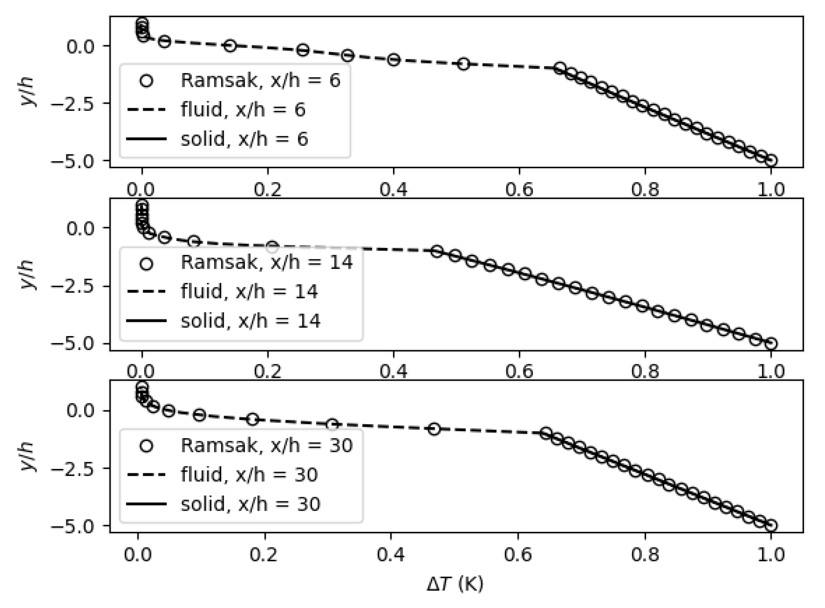
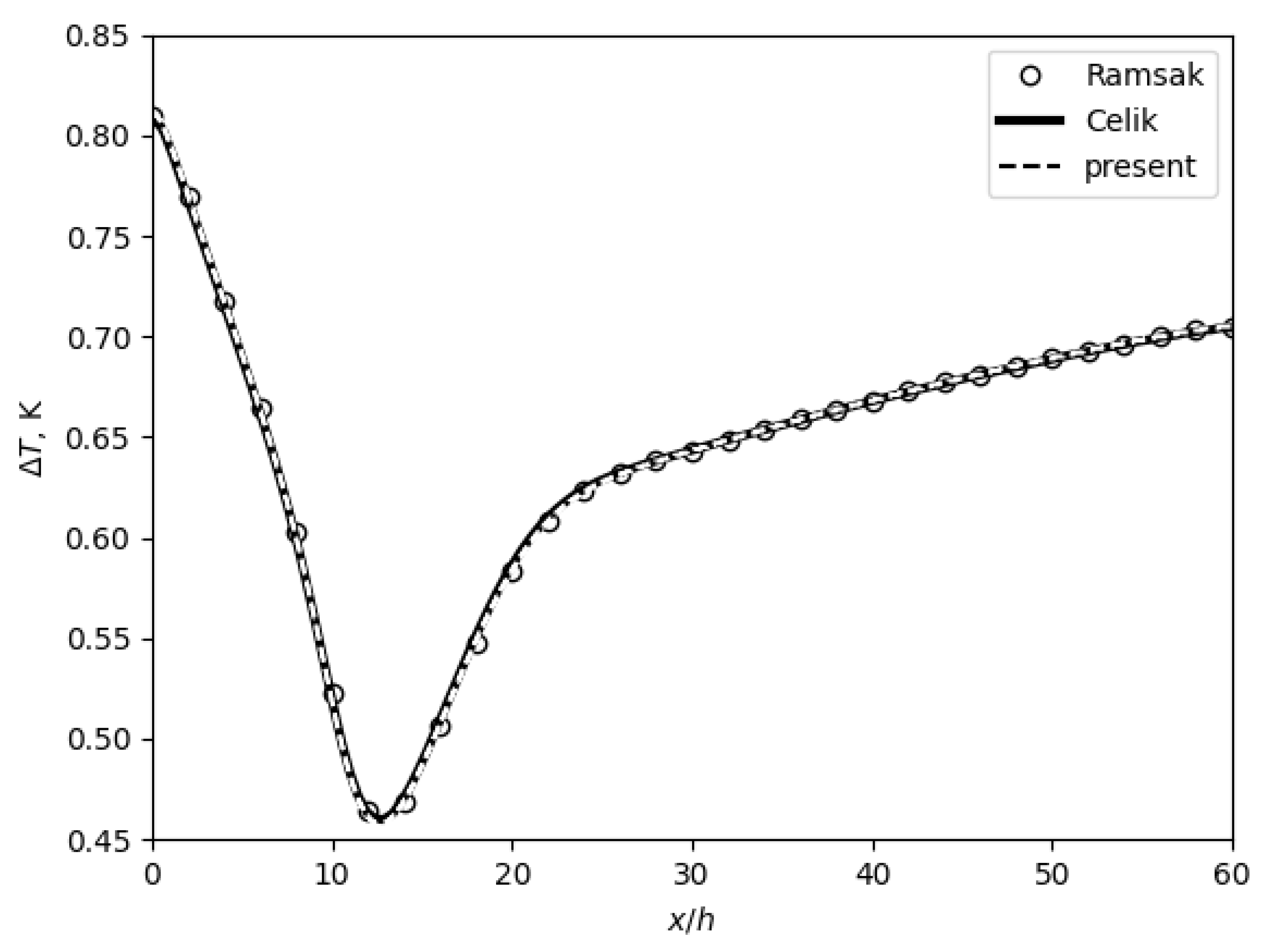
1.1.3. Backward-Facing Step with Downstream Heated Wall

The hydrodynamics of the backward-facing step have been studied extensively. The main parameters of interest are the Reynolds number, $Re$, and the step-to-channel height ratio, $S=s/h$. Here, the velocity used to calculate the value of $Re$ is the average velocity at the inlet, $\overline{U}$. Armaly et al. [21] considered a step with $S=4.9/5.2\approx 0.94231$, and found that with increasing $Re$, the length of the recirculation region downstream of the step increased in length. At about $Re=500$, a secondary separation region appeared on the upper channel wall, and the flow was seen to be three-dimensional for $400<Re<6600$. Similar behavior has been predicted in several other studies for example, [22,23].

The CHT in flow over a backward-facing step has received less attention. The main parameters which have been considered in the past are the same as for the hydrodynamics problem, with the addition of the normalized base thickness, $B=b/H$, the fluid Prandtl number, $Pr=\mu C/k$, and the solid-to-fluid thermal conductivity ratio, $\overline{k}=k_s/k$. Ramšak [24] simulated steady flow over a step with $S=1$ and $B=4$, for $Re=800$, $Pr=0.71$, a fixed temperature difference from ambient, $\Delta T=T-T_{\infty }=1$ K, and $\overline{k}=$ 1–1000. The results from solvers based on the boundary element and finite volume methods were in good agreement and it was found that the minimum temperature rose with increasing $\overline{k}$. Note that incompressible flow over a backward-facing step at $Re=800$ provides an extreme test for numerical models of the hydrodynamic part of the problem [25,26].

Celik [27] coupled separate finite volume solvers for the fluid and solid, with convergence based on the temperature and flux at the fluid–solid interface, obtaining good agreement with Ramšak’s results. The range of $Re$ was increased to 200–800 and the effects of $Pr$ and B were also examined: reducing $Re$ and $Pr$ caused the minimum temperature to increase, whilst not surprisingly, increasing B reduced the minimum temperature at the interface. Nouri-Borujerdi and Moazezi [28] obtained good agreement with the predictions from Ramšak’s calculations, as part of a study on the effect of obstacles on CHT.

1.1.4. More Complicated Problems

There are numerous examples of the conjugate heat transfer in industrial situations. Of relevance to the current problem of interest, there have been a number of studies of flows in microelectronic heat exchangers. For example, Yu and Joshi [29] compared experimental data with numerical results for a pin-fin heat sink located on one wall of a channel. This data was used for code validation by Balakin et al. [30]. Nakayama and Park [31] measured the temperature of a heated block mounted on the wall of a parallel plate channel at $Re=$ 2200–16,000. Two configurations were examined: heated block on adiabatic wall and adiabatic block on heated wall. They compared their temperature measurements on the wall with a two-dimensional finite difference model, finding good agreement for a range of different heat loads. Kumar et al. [32] used numerical CHT predictions to aid in material selection for a parallel microchannel heatsink.

It would appear, however, the problem of conjugate heat transfer in thermal inkjet printheads has not been considered previously, and so neither experimental data nor relevant simulation results are available. Thus, in an effort to understand and characterize this problem area, we have performed numerical simulations of the conjugate heat transfer in inkjet printhead geometries.

First, the numerical model is validated against theoretical solutions for the three relatively simple cases discussed above. For two of these, we derive analytical solutions in the next section. Then, the heating of the PHIC due to actuation, combined with the cooling due to nozzle refill from the ink supply, was simulated, with an investigation of the effect of the ink feed-hole width on the temperature field.

2. Theoretical Models

Here, we present the derivation of analytical expressions for two relatively simple cases: differentially heated, fully developed planar channel flow and forced convection against conduction.

2.1. Fully-Developed Planar Channel Flow with Forced Convection

Consider the fully developed forced convection with unidirectional flow in a plane duct with uniform transverse heat flux, Figure 2a.

Let $T(x,y)$ be the temperature at longitudinal position x along a duct $-h<y<h$ with a fully developed flow velocity profile $u\left(y\right)$ in the longitudinal direction. Assume that an overall uniform temperature gradient $\lambda x$ is imposed in the longitudinal direction by the boundary conditions $T(x,\pm h)=\lambda x\pm \Delta T$. The governing equation is:

$$\rho cu\left(y\right)\frac{\partial T}{\partial x}=k\frac{{\partial }^{2}T}{\partial y^2}$$

(3)

where k and $\rho c$ are the thermal conductivity and volumetric heat capacity of the fluid, respectively. Assuming a form inspired by analyses of fully developed forced convection in a uniformly heated tube [33,34],

$$T(x,y)=\lambda x+\frac{\Delta T}{h}y+\theta \left(y\right)$$

(4)

where the profile term $\theta \left(y\right)$ is to be determined. The one-dimensional profile satisfies

$$\lambda \rho cu\left(y\right)=k\frac{{\mathrm{d}}^2\theta }{\mathrm{d}{y}^2}$$

(5)

subject to boundary conditions $\theta (\pm h)=0$.

An expression for the solution as an integral over the general velocity profile u can be obtained from the method of undetermined coefficients [35] §3.6.1:

$$\begin{array}{ccccc}\hfill \theta \left(y\right)& =\hfill & \hfill \frac{-\lambda \rho c}{2hk}\left\{{\int }_{-h}^y(h-y)(h+\eta )u\left(\eta \right)\mathrm{d}\eta \right.& +\hfill & \hfill \left.{\int }_y^h(h+y)(h-\eta )u\left(\eta \right)\mathrm{d}\eta \right\}\end{array}$$

(6)

In the above, the temperature on the walls was specified as $T(x,\pm h)=\lambda x\pm \Delta T$, but the solution also corresponds to the case of uniform heat fluxes:

$$\begin{array}{cc}\hfill +k{\left.\frac{\partial T}{\partial y}\right|}_{y=+h}& =+k\left\{\frac{\Delta T}{h}+{\theta }^{\prime }(+h)\right\}\hfill \\ \hfill -k{\left.\frac{\partial T}{\partial y}\right|}_{y=-h}& =-k\left\{\frac{\Delta T}{h}+{\theta }^{\prime }(-h)\right\}.\hfill \end{array}$$

(7)

These do not cancel as heat is increasingly advected downstream if $\lambda >0$. The sum is:

$$k\left\{{\left.\frac{\partial T}{\partial y}\right|}_{y=+h}-{\left.\frac{\partial T}{\partial y}\right|}_{y=-h}\right\}=k{\left[\frac{\mathrm{d}\theta }{\mathrm{d}y}\right]}_{-h}^{+h}=\lambda \rho c{\int }_{-h}^{h}u\left(y\right)\mathrm{d}y$$

(8)

which is the product of the capacity rate per unit span and the streamwise component of the temperature gradient. Thus if the wall fluxes are specified, their sum determines the longitudinal gradient.

From Equation (6), we can see that ${\theta }^{\prime }(+h)+{\theta }^{\prime }(-h)$ vanishes when $u\left(y\right)=u(-y)$, as in Poiseuille flow. If the top wall heat transfer $q_{+h}=0$, then:

$$\begin{array}{cc}\hfill \lambda & =\frac{q_{-h}}{\rho c{\int }_{-h}^{h}u\left(y\right)\mathrm{d}y}\hfill \\ \hfill \Delta T& =\frac{-h{q}_{-h}}{2k}.\hfill \end{array}$$

(9)

For plane Poiseuille flow, $u\left(y\right)=u_0\left\{1-{(y/h)}^2\right\}$,

$$T(x,y)=\lambda x+\frac{\Delta T}{h}y-\frac{\lambda \rho c{u}_0}{12k{h}^2}\left(5h^2-y^2\right)\left(h^2-y^2\right)$$

(10)

The fluxes are related to:

$${\theta }^{\prime }(\pm h)=\frac{\mp 2\lambda \rho c{u}_{0}h}{3k}$$

(11)

Extension to Conjugate Heat Transfer

The exact solution can be extended to conjugate heat transfer by adding thickness to one of the walls and applying the heat flux there. The heat flux is uniform through the solid which has thermal conductivity $k_s$. Thus:

$$T(x,y)=\left\{\begin{array}{cc}\lambda x-\frac{q}{2k_{\mathrm{f}}}y+\theta \left(y\right),\hfill & -h<y<h;\hfill \\ \lambda x+q\left(\frac{h}{2k_{\mathrm{f}}}-\frac{h+y}{k_{\mathrm{s}}}\right),\hfill & y<-h,\hfill \end{array}\right.$$

(12)

and so, we obtain:

$$\theta (x,y<-h)=q(h+y)\left(\frac{1}{2k_{\mathrm{f}}}-\frac{1}{k_{\mathrm{s}}}\right)$$

(13)

2.2. One-Dimensional Transient Conduction against Convection

The solution for the problem of a step in superficial flux can be derived from that for the problem of a step in surface temperature (or rather antiderived, the latter being the derivative of the former). This was demonstrated by Carslaw and Jaeger [19], §2.9 for the special case $w=0$.

Say $N(z,t)$ were the solution of the partial differential equation together with the Neumann condition. Then

$$D\equiv \frac{-k{T}_{\mathrm{D}}}{q}\frac{\partial N}{\partial z}$$

(14)

would also be a solution of the partial differential equation but would satisfy the Dirichlet condition $D(0,t)=T_D$; therefore it must be the solution given by Carslaw and Jaeger [19], Equation (15.2.7), p. 388.

$$D=\frac{T_{\mathrm{D}}}{2}\left(\mathrm{erfc}\frac{z+wt}{2\sqrt{\alpha t}}+{\mathrm{e}}^{-wz/\alpha }\mathrm{erfc}\frac{z-wt}{2\sqrt{\alpha t}}\right)$$

(15)

where $\alpha =k/\rho C$ is the thermal diffusivity. This suggests seeking the antiderivative w.r.t. z of the solution of the Dirichlet problem:

$$N(z,t)=\frac{q}{k{T}_{\mathrm{D}}}{\int }_z^{\infty }D(\zeta ,t)\mathrm{d}\zeta$$

(16)

The first term can be integrated by substitution with $2{\left(\alpha t\right)}^{1/2}y=\zeta +wt$ and expressed using the iterated integral of the complementary error function [19], Equation (2.1.7), p. 51:

$$\frac{1}{2}{\int }_z^{\infty }\mathrm{erfc}\frac{\zeta +wt}{2\sqrt{\alpha t}}\mathrm{d}\zeta =\sqrt{\alpha t}\mathrm{ierfc}\frac{z+wt}{2\sqrt{\alpha t}}$$

(17)

The second term can be integrated by parts:

$$\begin{array}{c}\frac{1}{2}{\int }_z^{\infty }{\mathrm{e}}^{-w\zeta /\alpha }\mathrm{erfc}\frac{\zeta -wt}{2\sqrt{\alpha t}}\mathrm{d}\zeta \hfill \\ =\frac{\alpha }{2w}\left\{{\mathrm{e}}^{-wz/\alpha }\mathrm{erfc}\frac{z-wt}{2\sqrt{\alpha t}}-\mathrm{erfc}\frac{z+wt}{2\sqrt{\alpha t}}\right\}\hfill \end{array}$$

(18)

Thus the solution of the problem with step heat-flux is:

$$T(z,t)=\frac{q}{k}\left\{\sqrt{\alpha t}\mathrm{ierfc}\frac{z+wt}{2\sqrt{\alpha t}}+\frac{\alpha }{2w}\left[{\mathrm{e}}^{-wz/\alpha }\mathrm{erfc}\frac{z-wt}{2\sqrt{\alpha t}}-\mathrm{erfc}\frac{z+wt}{2\sqrt{\alpha t}}\right]\right\}$$

(19)

Of interest in applications is the superficial temperature:

$$T(0,t)=\frac{q}{\rho cw}\left(2\sqrt{\tau }\mathrm{ierfc}\sqrt{\tau }+\mathrm{erf}\sqrt{\tau }\right)$$

(20)

where we have introduced the dimensionless time $\tau \equiv \frac{w^{2}t}{4\alpha }$. Making use of the asymptotic expansion:

$$\mathrm{erfc}t\sim \frac{{\mathrm{e}}^{-t^2}}{t\sqrt{\pi }},t\to \infty$$

(21)

and its implication

$$\mathrm{ierfc}t\sim \frac{{\mathrm{e}}^{-t^2}}{\sqrt{\pi }},t\to \infty$$

(22)

the eventual form of the solution is:

$$T(z,\infty )\sim \frac{q}{\rho cw}{\mathrm{e}}^{-4\zeta }$$

(23)

where we have introduced the normalized coordinate $\zeta \equiv wz/4\alpha$. In particular, the eventual superficial temperature is $T(0,\infty )\approx q/\rho cw$.

3. Methods

3.1. Equations for Advection–Diffusion

Simulations are performed using the OpenFOAM conjugate heat transfer solver, chtMultiRegionFoam. For fluid regions, the compressible continuity (24), momentum (25) and energy (26) equations are solved [33,36,37,38]:

$$\nabla ·\left(\rho \mathbf{U}\right)=0$$

(24)

$$\frac{D\left(\rho \mathbf{U}\right)}{Dt}=-\nabla p+\nabla ·\mu \left(\nabla \mathbf{U}+\nabla {\mathbf{U}}^{\mathrm{T}}\right)+\mathbf{F}$$

(25)

$$\begin{array}{c}\hfill \frac{\partial \rho H}{\partial t}+\nabla ·\left(\rho \mathbf{U}H\right))+\frac{\partial \rho K}{\partial t}+\nabla ·\left(\rho \mathbf{U}K\right)-\frac{\partial p}{\partial t}\\ \hfill =-\nabla ·\mathbf{q}+\rho S+\nabla ·\left(\sigma ·\mathbf{U}\right)\end{array}$$

(26)

Here, $\mathbf{U}$ = velocity, p = pressure, $\mu$ = viscosity, $\mathbf{F}$ = body force, H = specific enthalpy, K = specific kinetic energy, $\mathbf{q}$ = heat flux, S = heat generation and $\sigma$ = fluid shear. These equations are completed by the perfect gas law.

For the current problems of interest, the flow is nonreacting, radiation effects are unimportant and buoyancy effects can be neglected: the Grashof number $Gr=g\beta \Delta T{H}^3/{\nu }^2$ $\ll 0.1$. Here, g is gravitational acceleration, $\beta$ is coefficient of thermal expansion of the fluid, $\Delta T$ is the difference between the surface and ambient temperature values. We focus on relatively low Reynolds number flows, for instance, in the common printhead supply channel above the inkjet actuators, $Re\approx 1$.

Inside solid regions, the energy equation is solved [33,36,37,38]:

$$\frac{\partial \left(\rho H\right)}{\partial t}=\nabla ·\left(\nabla \alpha H\right)+S_h$$

(27)

where $S_h$ = source terms.

3.2. Solvers, Discretization and Boundary Conditions

The transient terms are solved using backward Euler time stepping, whilst the spatial terms are discretized using second order centred-differencing. Pressure coupling is achieved using the PISO method. The pressure equation is solved using the geometric–algebraic multigrid method. The velocity and energy equations are solved using the preconditioned stabilized conjugate gradient method. Further details of the methods are given in [39,40].

In fluid regions, no-slip velocity boundary conditions are applied at the walls [33,36,37], together with zero pressure-gradient boundary conditions [38,39]. At inlets, the velocity profile is specified together with a zero pressure gradient; at outlets, the normal velocity gradient is zero, the tangential value is also zero and the pressure is fixed. For the solid regions [33,36,37,38], the walls are treated differently depending on the type of boundary condition: insulated walls have a zero temperature gradient, whilst walls that are heated have a fixed gradient equal to the heat flux divided by the adjacent material thermal conductivity; a fixed temperature boundary is applied to the bottom wall of the backward-facing step, with $\Delta T=1$ K. The temperature profile at the inlet is set either as constant or as a function of distance from the walls, whilst at outlets, zero temperature gradient is specified.

In the chtMultiRegionFoam solver, overall convergence of the solution is judged to have occurred when convergence is achieved in each of the different regions. That is, there is no specific check for consistency in temperature and heat flux at the boundary, which is the typical approach, see [24,27,28]. The boundary conditions are part of the solution matrix and thus contribute to the overall residual. Considering that the residuals are normalized and the boundary condition may only make a minor contribution, the strategy does not necessarily mean that the interface conditions are converged when the individual solutions are judged to be so. To ensure that convergence is met, it was found that specifying residual tolerances of ${10}^{-5}$ for the pressure, velocity and energy equations gave converged interface thermal boundary conditions with residual differences in the interface temperature and heat flux values of less than ${10}^{-4}$.

4. Results

4.1. Comparison with Analytical Models

The predicted temperature profile for Poiseuille flow in a channel with one wall attached to a solid, heated at its outer surface, is compared with the analytical expression, Equation (13) in Figure 3. The fluid properties are those of water: $\rho c=4.181\times {10}^6$ J m${}^{-3}$ K${}^{-1}$, $\mu =1$ mPa s, and $k=0.5856$ W m${}^{-1}$ K${}^{-1}$, giving a Prandtl number value of $Pr=7.14$. The solid properties are $\rho c=3.6\times {10}^6$ J m${}^{-3}$ K${}^{-1}$ and $k=80$ W m${}^{-1}$ K${}^{-1}$. The channel height and length are 0.1 mm and 1 mm, respectively, the downstream solid wall thickness is 0.05 mm, the maximum velocity is 1 m s⁻¹, and the heat flux applied to the lower wall divided by the fluid thermal conductivity is 100 K/mm. The Reynolds number based on channel height is $Re=100$, and the Peclet number is $Pe\approx 714$. The comparison is good, and computations for different values of $Re$ and $Pe$ show similar good agreement. The difference between the analytical model and the numerical results is summarized in

Table 1. Average difference between analytical and numerical results for temperature profile at the outlet, for different mesh sizes.

Mesh Size/Channel Height	(${\mathit{T}}_{\mathit{a}}$−${\mathit{T}}_{\mathit{n}}$)/${\mathit{T}}_{\mathit{a},\mathit{m}\mathit{a}\mathit{x}}$ (%)
0.17	0.69
0.1	0.49
0.05	0.39
0.025	0.35

for a range of different mesh sizes. Here, the difference is evaulated for the profile at the end of the channel, and is averaged over all of the points in the profile for each mesh. Even for fairly coarse meshes, the numerical simulations agree with the analytical values to within less than one percent, and reducing the mesh size reduces the error value.

For conduction against convection, Equation (20), we performed a series of simulations using a varying mesh size, with the time step adjusted to keep the Fourier number, $Fo=\alpha \Delta t/\Delta x^2$, fixed. The error was calculated in the same way as for the channel problem, discussed above. The comparison shown in Figure 4 suggests that the numerical model is in good agreement with the analytical solution, and that small errors can be achieved with relatively coarse meshes.

4.2. Backward-Facing Step

The two-dimensional simulation domain extended a distance equal to sixty times the step height downstream of the step, as testing showed that the results did not change with further increases in this distance. The mesh was uniform with edge length equal to one-twentieth of the channel height. Mesh refinement was performed and the difference between the established results for separated length and interface temperature distribution were calculated, the latter being averaged over all the points in the profile, as was done in the previous section.

Initial simulations of the hydraulics at $Re=800$ were performed using simpleFoam, and it was found that the computed separation and reattachment points were in good agreement with earlier studies: the reattachment point on the lower wall, $x_1/h=12.2$, compared with 12.22 reported by Gartling [25] and 12.2 by Ramšak [24]; the separation and reattachment points on the upper wall $x_2/h=9.70$ and $x_3/h=20.9$, respectively, compared with 9.70 and 21.0 reported by Gartling and 9.75 and 21.0 by Ramšak. It should be noted that a mesh size of one-fourtieth of the incoming channel height was required to obtain a converged solution without resorting to numerical stabilization.

Next, simulations were performed using chtMultiRegionFoam for the same value of $Re$ and for solid-to-fluid thermal conductivity ratio, $\overline{k}=10$, as per [24,27]. We found that the solver had difficulty converging if both fluid and solid regions were solved together. So, we took the following approach: first, solve for the fluid region with no heat applied; then, using this velocity field, solve the energy equation without solving for the flow.

The predictions for temperature profiles at three locations considered by Ramšak for $Re=800$ are shown in Figure 5 whilst the interface profiles are compared in Figure 6 together with the values from Celik. The present simulations are in good agreement with the earlier work. Further comparisons with Celik’s results are shown in Figure 7, for $Re=$ 200, 400 and 600 with $\overline{k}=10$, and for $\overline{k}=$ 1, 10 and 100 for $Re=200$. Once again, the comparison between the values is good. The average difference between the computed interface temperature profile, using a cell size of one-fourtieth of the incoming channel height, and the results from Ramšak was approximately 0.04%.

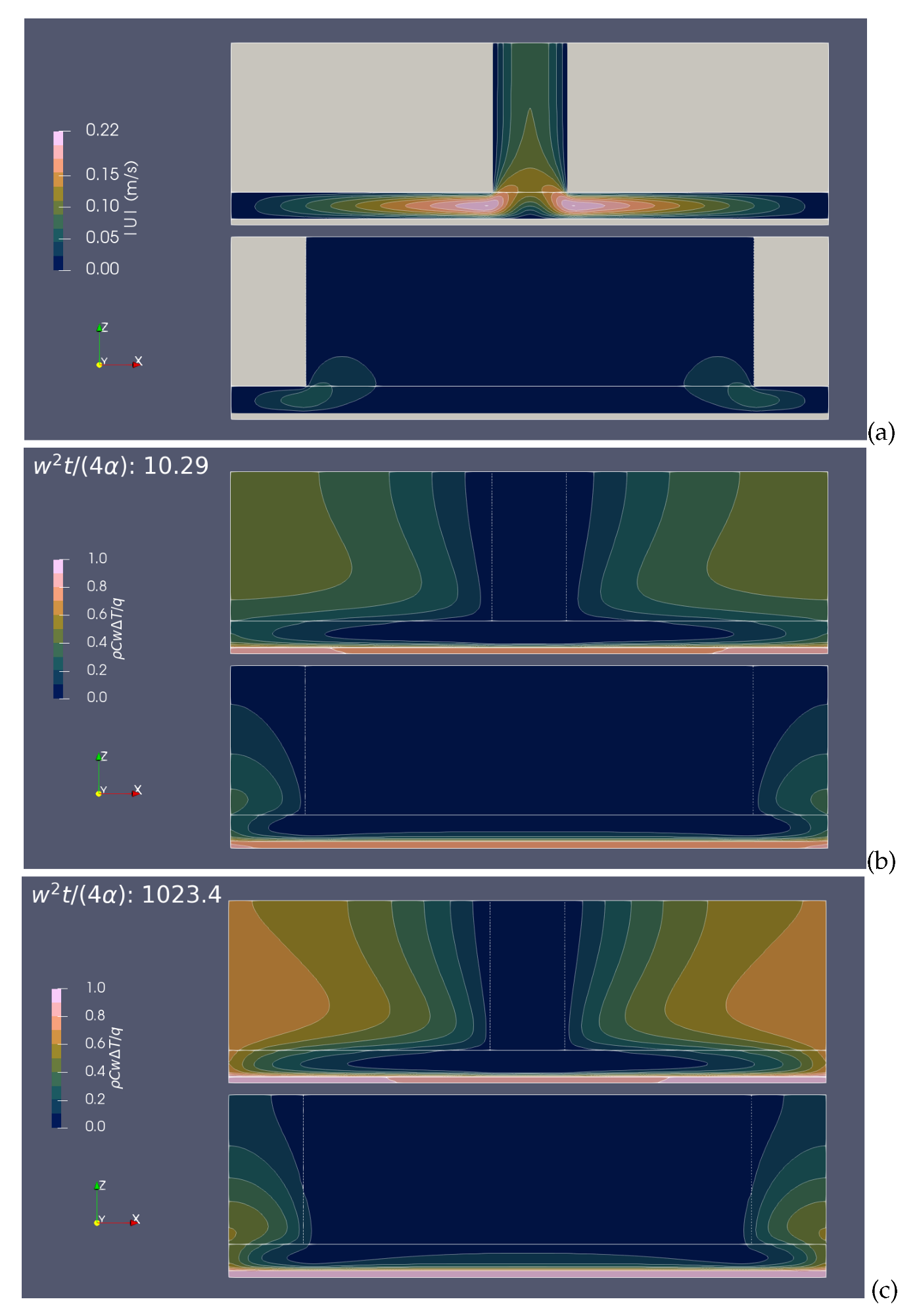
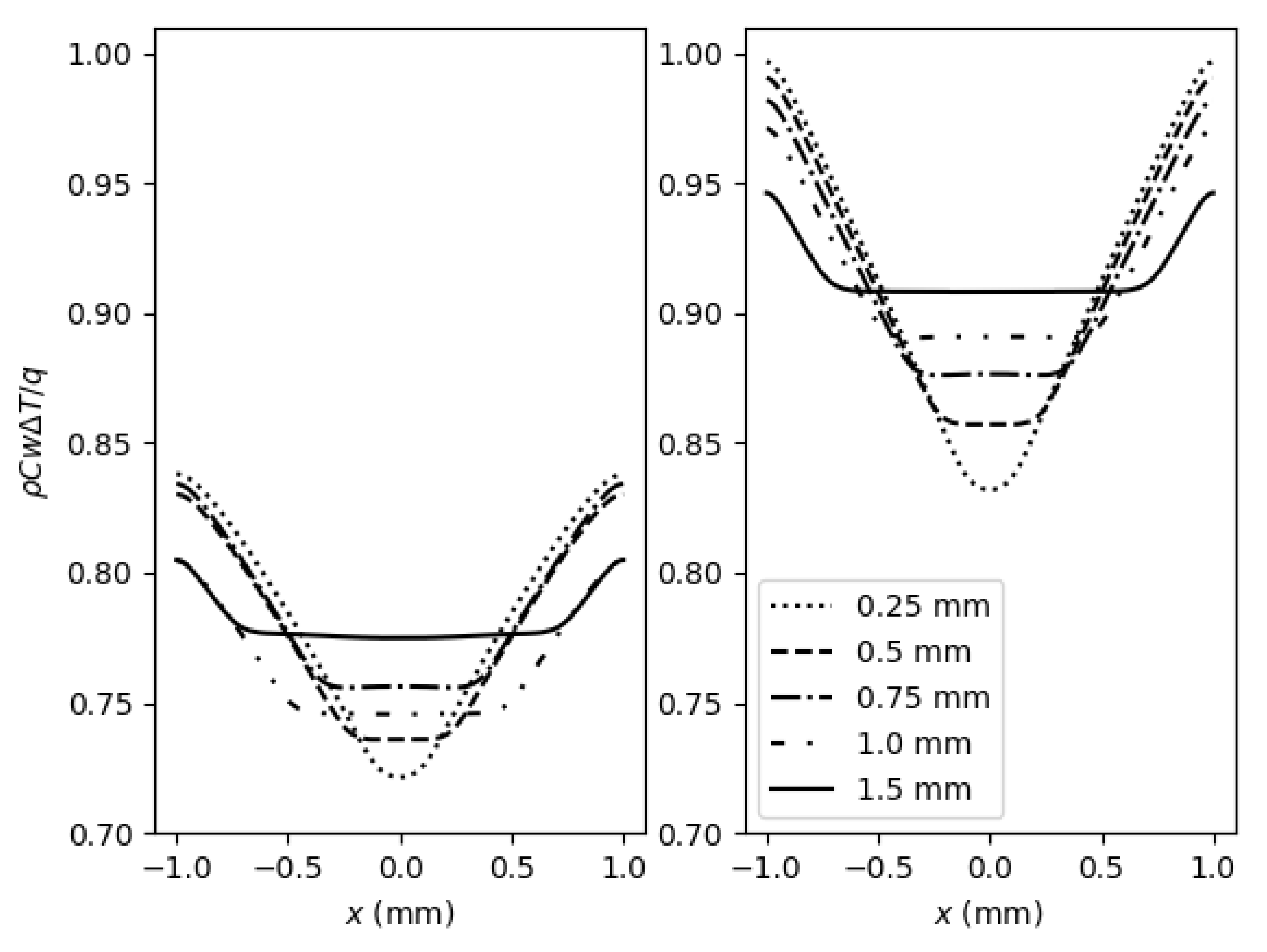
4.3. Thermal Inkjet Printhead

It was noticed that the printed image density produced by regions of the chip located directly below ink feed holes was significantly lighter than those regions directly adjacent. This is due to the lower temperature in those regions, caused by the greater cooling due to the flow caused by chamber refill. In turn, this reduces the droplet volume and thus the printed image density. The problem at hand is to limit the difference between the maximum and minimum temperature values experienced by the actuators.

Inkjet printheads are typically comprised of a number of different materials, with large differences in material properties, especially thermal conductivity, for which the difference can exceed two orders of magnitude, see

Table 2. Material properties for printhead model. Note that all properties are assumed to be invariant with temperature.

Material	$\mathit{\rho }$ (kg m${}^{-3}$)	c (J kg${}^{-1}$ K${}^{-1}$)	k (W m${}^{-1}$ K${}^{-1}$)	$\mathit{\mu }$ (mPa s)	Source
ink	1050	4181	0.6	3.0	in house
silicon	2330	702.24	153	-	[41,42]
plastic	1500	1250	0.3	-	manufacturer

. For the ink, the density and viscosity were measured in-house, using a balance and a spindle viscometer, respectively. The specific heat and thermal conductivity are assumed to be those of water. The values for silicon come from Shackelford and Alexander [41] (density and specific heat) and Touloukian et al. [42] (thermal conductivity). We have tested a number of different plastic materials, and the values shown are typical of those supplied by manufacturers.

Ink passages in some of the layers cause complex flows to develop. Here we will consider a relatively simple geometry where flow enters the main ink conduit above the MEMS via a hole in a plastic connecting layer, see Figure 8a for a schematic. Heat is added to the MEMS layers due to the thermal inkjet actuator operation; at the same time, the back side of the MEMS is cooled by the refill flow, which is modelled as a steady plug profile for simplicity. The geometry plus a close-up view of the mesh are presented in Figure 8b,c, respectively. Given that the flow of cool ink is causing the temperature difference, it was decided to investigate the effect of reducing the flow velocity by increasing the ink feedhole width, $W_h$. The initial design had $W_h=0.25$ mm, with a center-to-center spacing of 2 mm; hole width values of 0.5, 0.75, 1.0 and 1.5 mm were also considered.

The steady velocity field, due to refill of the thermal inkjet actuators (Figure 9a), is solved first, without the addition of heat. The specified refill velocity, w, is determined from the average flow rate, Q, due to refilling chambers with the ejected droplet volume, V, at the firing frequency, f. Here, $w=Q/A=nVf/A$, where A is the cross-sectional area of the back etch channel. For the current study, we assumed $w=0.0239$ m s${}^{-1}$. After computing the velocity field, the heating is activated and we freeze the flow, only solving the heat equation in the solid and fluid materials. We apply the heat as a volumetric source in the bottom-most layer of the silicon mesh, which has a thickness of 5 μ$\mathrm{m}$. The heat load is computed as the average power density applied to each actuator. This amounts to $27.3$ kW mm${}^{-3}$.

The instantaneous contour plots of velocity magnitude and temperature rise at nondimensional times $w^{2}t/\left(4\alpha \right)=10.29$ and $1023.4$ are shown in Figure 9 for the smallest and largest values of hole width, $W_h=0.25$ and $1.5$ mm. The velocity field results shows that narrow width hole increases the peak velocity. There is a strong turning of the flow near the corner, and the peak velocity at each x-station decays with distance from the center of the feedhole. The temperature results show that the heat spreads fairly evenly along the MEMS (silicon) layer, and only partially into the less thermally conductive ink and plastic layers. As the flow slows with increasing distance from the center-line, conduction through the ink raises the temperature; this is aided by conduction through the silicon sidewalls. The temperature in the silicon is much more uniform than in the other components.

The temperature profile along an x-transect at the bottom of the silicon is shown, in Figure 10, at two different times after the start of printing at $t=0$, for the five different hole width values considered. It is clear that the narrower hole provides the greatest difference, $\delta$, between minimum and maximum temperature difference; the variation of $\delta$ with time is shown in Figure 11. The difference rises to achieve a steady value soon after the start of printing.

It is of interest to see how the temperature in the complete model compares with the one-dimensional solution from Section 2.2. We repeated the full three-dimensional calculation with the solid plastic component set to be a flowing ink component, and with both the solid plastic and silicon components set as ink. Figure 12 shows the average temperature at the ink–silicon interface as a function of time for the widest hole, $W_h=1.5$ mm, together with the results from simulation models where the plastic and all solids (plastic plus silicon) have been changed to ink. Also shown is the one-dimensional analytical model, Equation (20). It can be seen that the full three-dimensional simulation model takes much longer to reach a steady state than the one-dimensional result; similar behavior is also seen with the two other models with progressively less solids. As expected, the model without solids matches the one-dimensional analytical result: the simulation model in that case consists only of heat applied to the bottom of an ink layer, as per the theory. The extra solid components add not only pathways for heat to leak through instead of the ink, but also cause the flow to undergo deceleration and changes in direction which enhance the heat transfer, thus lowering the temperature at the bottom of the silicon.

5. Conclusions and Future Work

Simulations of conjugate heat transfer in a thermal inkjet printhead have been performed. In particular, the effect of changing the width of the ink feedhole, located directly above the printhead chip, on the temperature uniformity in the chip has been examined. The simulation method was validated against analytical models derived herein, and with earlier simulations of conjugate heat transfer in flow over a backward-facing step. Using the validated simulation model, it was found that increasing the ink feedhole width reduces the difference between the maximum and minimum temperature in the prinhead chip, thus reducing any droplet volume and image density differences. It was also found that for the inkjet printer problem, the peak temperature is somewhat lower than predicted using the one-dimensional analytical model for conduction against convection, and that this seems to be due to leakage of thermal energy from the heated area into the silicon.

A weakness of the present study is the lack of experimental data for comparison with the simulation model. The printhead chips available for testing currently have thermocouples embedded in them with a spacing of approximately 2 mm. This is not suitable for investigating problems with thermal lengthscales of order 0.01–1 mm, as in the current study. Adding extra sensors to the printhead chips would be expensive, and so would need to be justified on the grounds of product improvement rather than providing experimental data for testing theoretical models. Infrared thermography is another option, which could provide a means of obtaining experimental data at the right length and time scales. Such an apparatus is expensive, and so it would likely be necessary to establish a collaboration with a research center that has this tool available to be used.

References

1. Graetz, L. Ueber die Wärmeleitungsfähigkeit von Flüssigkeiten. Ann. Der Phys. Und Chem. 1885, 25, 337–357. [Google Scholar] [CrossRef]
2. Papoutsakis, E.; Ramkrishna, M. Conjugated Graetz problems—I: General formalism and a class of solid-fluid problems. Chem. Eng. Sci. 1981, 36, 1381–1391. [Google Scholar] [CrossRef]
3. White, F.M. Viscous Fluid Flow, 2nd ed.; McGraw-Hill: New York, NY, USA, 1991. [Google Scholar]
4. Sugavanam, R.; Ortega, A.; Choi, C.Y. A numerical investigation of conjugate heat transfer from a flush heat source on a conductive board in laminar channel flow. Int. J. Heat Mass Transf. 1995, 38, 2969–2984. [Google Scholar] [CrossRef]
5. Wansophark, N.; Malatip, A.; Dechaumphai, P. Streamline upwind finite element method for conjugate heat transfer problems. Acta Mech. Sin. 2005, 21, 436–443. [Google Scholar] [CrossRef]
6. Mori, S.; Sakakibara, M.; Tanimoto, A. Steady laminar heat transfer in a circular tube with conduction in tube wall. Chem. Eng. 1974, 38, 144–150. [Google Scholar] [CrossRef]
7. Sucec, J. Unsteady conjugated forced convective heat transfer in a duct with convection from the ambient. Int. J. Heat Mass Transf. 1987, 30, 1963–1970. [Google Scholar] [CrossRef]
8. Yan, W.M.; Tsay, Y.L.; Lin, T.F. Transient conjugated heat transfer in laminar pipe flows. Int. J. Heat Mass Transf. 1989, 32, 775–777. [Google Scholar] [CrossRef]
9. Nagendra, K.; Tafti, D.K.; Viswanath, K. A new approach for conjugate heat transfer problems using immersed boundary method for curvilinear grid based solvers. J. Comp. Phys. 2014, 267, 225–246. [Google Scholar] [CrossRef]
10. Sucec, J.; Sawant, A.M. Unsteady, conjugated, forced convection heat transfer in a parallel plate duct. Int. J. Heat Mass Transf. 1984, 27, 95–101. [Google Scholar] [CrossRef]
11. Karvinen, R. Transient conjugated heat transfer to laminar flow in a tube or channel. Int. J. Heat Mass Transf. 1988, 31, 1326–1328. [Google Scholar] [CrossRef]
12. Gallegos-Muñoz, A.; Balderas-Bernal, J.A.; Violante-Cruz, C.; Rangel-Hernández, V.H.; Belman-Flore, J.M. Analysis of the conjugate heat transfer in a multi-layer wall including an air layer. Appl. Therm. Eng. 2010, 30, 599–604. [Google Scholar]
13. Omosehin, O.S.; Adelaja, A. Numerical simulation of conjugate heat transfer in forced convective boundary bilayered cylindrical pipe with different Peclet numbers. Fed. Univ. Oye-Ekiti J. Eng. Tech. 2019, 4, 158–163. [Google Scholar] [CrossRef]
14. Bilir, Ş.; Ateş, A. Transient conjugated heat transfer in thick walled pipes with convective boundary conditions. Int. J. Heat Mass Transf. 2003, 46, 2701–2709. [Google Scholar] [CrossRef]
15. Manna, P.; Chakraborty, D. Numerical investigation of conjugate heat transfer problems. Indian J. Aerosp. Sci. Tech. 2004, 56, 166–175. [Google Scholar]
16. Mason, M.; Weaver, W. The settling of small particles in a fluid. Phys. Rev. 1924, 23, 412–426. [Google Scholar] [CrossRef]
17. Pérez Guerrero, J.S.; Pimentel, L.C.G.; Skaggs, T.H.; van Genuchten, M.T. Analytical solution of the advection–diffusion transport equation using a change-of-variable and integral transform technique. Int. J. Heat Mass Transf. 2009, 52, 3297–3304. [Google Scholar] [CrossRef]
18. Wang, J.; Shao, M.; Huang, L.; Jia, X. A general polynomial solution to convection–dispersion equation using boundary layer theory. J. Earth Syst. Sci. 2017, 126, 40. [Google Scholar] [CrossRef] [Green Version]
19. Carslaw, H.S.; Jaeger, J.C. Conduction of Heat in Solids, 2nd ed.; Oxford University Press: Oxford, UK, 1959. [Google Scholar]
20. van Genuchten, M.T.; Alves, W.J. Analytical Solutions of the One-Dimensional Convective-Dispersive Solute Transport Equation; Tech. Bull. number 1661; U. S. Salinity Laboratory, Agricultural Research Service, United States Department of Agriculture: Washington, DC, USA, 1982. [Google Scholar]
21. Armaly, B.F.; Durst, F.; Pereira, J.C.F.; Schonung, B. Experimental and theoretical investigation of backward-facing step flow. J. Fluid Mech. 1983, 127, 473–496. [Google Scholar] [CrossRef]
22. Biswas, G.; Breuer, M.; Durst, F. Backward–facing step flows for various expansion ratios at low and moderate Reynolds numbers. J. Fluids Eng. 2004, 126, 362–374. [Google Scholar] [CrossRef]
23. Kaiktsis, L.; Karniadakis, G.E.; Orsz, S.A. Onset Three-Dimens. Equilibria, Early Transit. Flow A Backward-Facing Step. J. Fluid Mech. 1991, 231, 501–528. [Google Scholar] [CrossRef] [Green Version]
24. Ramšak, M. Conjugate heat transfer of backward-facing step flow: A benchmark problem revisited. Int. J. Heat Mass Transf. 2015, 84, 791–799. [Google Scholar] [CrossRef]
25. Gartling, D.K. A test problem for outflow boundary conditions - flow over a backward-facing step. Int. J. Num. Methods Fluids 1990, 11, 953–967. [Google Scholar] [CrossRef]
26. Gresho, P.M.; Gartling, D.K.; Torczynski, J.R.; Cliffe, K.A.; Winters, K.H.; Garratt, T.J.; Spence, A.; Goodrich, J.W. Is the steady viscous incompressible two-dimensional flow over a backward-facing step at Re = 800 stable? Int. J. Num. Methods Fluids 1993, 17, 501–541. [Google Scholar] [CrossRef]
27. Celik, B. Conjugate heat transfer characteristics of laminar flows through a backward facing step duct. Süleyman Demirel Univ. Inst. Sci. Tech. Mag. 2017, 21, 820–830. [Google Scholar] [CrossRef]
28. Nouri–Borujerdi, A.; Moazezi, A. Investigation of obstacle effect to improve conjugate heat transfer in backward facing step channel using fast simulation of incompressible flow. Heat Mass Transf. 2018, 54, 135–150. [Google Scholar] [CrossRef]
29. Yu, E.; Joshi, Y. Heat transfer enhancement from enclosed discrete components using pin-fin heat sinks. Int. J. Heat Mass Transf. 2002, 45, 4957–4966. [Google Scholar] [CrossRef]
30. Balakin, V.; Churbanov, A.; Gavriliouk, V.; Makarov, M.; Pavlov, A. Verification and validation of EFD.lab code for predicting heat and fluid flow. In CHT-04-Advances in Computational Heat Transfer III. Proceedings of the Third International Symposium; Begel House Inc.: Danbury, CT, USA, 2004. [Google Scholar]
31. Nakayama, W.; Park, S.-H. Conjugate heat transfer from a single surface-mounted block to forced convective air flow in a channel. J. Heat Transf. 1996, 118, 301–309. [Google Scholar] [CrossRef]
32. Kumar, A.U.; Javed, A.; Dubey, S.K. Material selection for microchannel heatsink: Conjugate heat transfer simulation. IOP Conf. Ser. Mater. Sci. Eng. 2018, 346, 012024. [Google Scholar] [CrossRef]
33. Bird, R.B.; Stewart, W.E.; Lightfoot, E.N. Transport Phenomena, 2nd ed.; Wiley: New York, NY, USA, 1960. [Google Scholar]
34. Eckert, E.R.G.; Gross, J.F. Introduction to Heat and Mass Transfer. McGraw-Hill Series in Mechanical Engineering; McGraw-Hill: New York, NY, USA, 1963. [Google Scholar]
35. Boyce, W.E.; DiPrima, R.C. Elementary Differential Equations and Boundary Value Problems, 2nd ed.; John Wiley & Sons: New York, NY, USA, 1969. [Google Scholar]
36. Dorfman, A.S. Conjugate Problems in Convective Heat Transfer; CRC Press: Boca Raton, FL, USA, 2010. [Google Scholar]
37. Faghri, A.; Zhang, Y.; Howell, J. Advanced Heat and Mass Transfer; Global Digital Press: Columbia, MO, USA, 2010. [Google Scholar]
38. Greenshields, C.J. Energy Equation in OpenFOAM. Available online: https://cfd.direct/openfoam/energy-equation/ (accessed on 16 November 2022).
39. Greenshields, C.J.; Weller, H.G. Notes on Computational Fluid Dynamics: General Principles; CFD Direct Limited: Reading, UK, 2022. [Google Scholar]
40. Holzmann, T.; Nagy, J. Mathematics, Numerics, Derivations and OpenFOAM; Holzmann CFD: Augsburg, Germany, 2021. [Google Scholar]
41. Shackelford, J.F.; Alexander, W. (Eds.) CRC Materials Science and Engineering Handbook; CRC Press: Boca Raton, FL, USA, 2001. [Google Scholar]
42. Touloukian, Y.S.; Powell, R.W.; Ho, C.Y.; Klemens, P.G. Thermal Conductivity—Metallic Elements and Alloys; Thermophysical Properties of Matter; Plenum: New York, NY, USA, 1970; Volume 1. [Google Scholar]
Figure 1. Flow in the printhead is driven by refill of the chambers in the MEMS layer. The nozzles at the bottom of the image experience a capillary suction pressure which is inversely proportional to the nozzle length scale. This capillary pressure draws ink from locations above the MEMS, via the feedhole in the plastic printhead layer.
Fluids 08 00088 g001
Figure 2. Schematics of problems exhibiting similar physical behavior as the full problem. (a) Fully developed forced convection and conjugate heat transfer in a planar channel. (b) One-dimensional conduction against convection. (c) Backward-facing step flow with a heated downstream wall. Note that analytical solutions are derived here for cases (a,b).
Fluids 08 00088 g002
Figure 3. Comparison of temperature rise predictions at the outlet plane, x = L , using chtMultiRegionFoam and theory for Poiseuille profile.
Fluids 08 00088 g003
Figure 4. Comparison of temperature rise predictions using chtMultiRegionFoam and theory for one-dimensional conduction against convection, for a variety of different mesh sizes, holding the Fourier number constant.
Fluids 08 00088 g004
Figure 5. Comparison of temperature profiles at three locations downstream of the step, R e = 800 , P r = 0.71 , k ¯ = 10 .
Fluids 08 00088 g005
Figure 6. Comparison of temperature profiles at the fluid-solid interface.
Fluids 08 00088 g006
Figure 7. Comparison of predicted temperature profiles and results from Celik at the fluid–solid interface for varying R e (a) and k ¯ (b).
Fluids 08 00088 g007
Figure 8. Geometry and mesh. (a) schematic showing main dimensions: W = width, t = thickness, = length, subscripts ‘i’ = ink, ‘p’ = plastic, ‘s’ = silicon, ‘m’ = MEMS, ‘w’ = plastic side-wall; for these simulations, W h is varied from 0.25 to 1.5 mm, whilst the following parameters are held constant: W p = 2 mm, t p = 0.5 mm, t s = 0.11 mm, t m = 0.02 mm, p = 0.25 mm, w = 0.05 mm, m = 0.09 mm; (b) the simulation domain is composed of three materials: blue = silicon, red = ink, green = plastic; (c) mesh on symmetry plane at y = 0 , showing refinement provided by snappyHexMesh.
Fluids 08 00088 g008
Figure 9. Velocity magnitude and printhead temperature rise on symmetry plane. (a) steady flow velocity magnitude; (b) temperature rise, w 2 t / ( 4 α ) = 10.29 ; (c) temperature rise, w 2 t / ( 4 α ) = 1023.4 .
Fluids 08 00088 g009
Figure 10. Temperature profile along x-transect at bottom of silicon at y = 0 . Left: w 2 t / ( 4 α ) = 10.29 ; Right: w 2 t / ( 4 α ) = 1023.4 .
Fluids 08 00088 g010
Figure 11. Difference, δ , between maximum and minimum temperature along x-transect at the bottom of the silicon component, that is, the print-face, at y = 0 for different values of hole width, W h .
Fluids 08 00088 g011
Figure 12. Average silicon temperature for printhead.
Fluids 08 00088 g012