Article

A Highly Scalable Direction-Splitting Solver on Regular Cartesian Grid to Compute Flows in Complex Geometries Described by STL Files

1
Department of Mathematics, University of British Columbia, Vancouver, BC V6T 1Z2, Canada
2
Department of Chemical and Biological Engineering, University of British Columbia, Vancouver, BC V6T 1Z3, Canada
*
Author to whom correspondence should be addressed.
Fluids 2023, 8(3), 86; https://doi.org/10.3390/fluids8030086
Submission received: 30 December 2022 / Revised: 21 February 2023 / Accepted: 23 February 2023 / Published: 28 February 2023
(This article belongs to the Special Issue Advances in Numerical Methods for Multiphase Flows, Volume II)

Abstract

:
We implement the Direction-Splitting solver originally proposed by Keating and Minev in 2013 and allow complex geometries to be described by a triangulation defined in STL files. We develop an algorithm that computes intersections and distances between the regular Cartesian grid and the surface triangulation using a ray-tracing method. We thoroughly validate the implementation on assorted flow configurations. Finally, we illustrate the scalability of our implementation on a test case of a steady flow through 144,327 spherical obstacles randomly distributed in a tri-periodic box at R e = 19.2 . The grid comprises 6.8 billion cells and the computation runs on 6800 cores of a supercomputer in less than 48 h.

1. Introduction

The quest for accurate and fast fluid flow solvers has been an on going concern in the Computational Fluid Dynamics community for years. Regardless of the complex nature of the fluid flow such as multiphase, non-Newtonian, with heat transfer or turbulent, the core of a flow solver involves solving the coupled conservation of mass and conservation of momentum on a grid with additional source/sink terms related to the complexity of the flow. With the rise of supercomputing over the last 20 years, high scalability has become the third important property that modern fluid flow solvers must satisfy. Assuming that the flow is incompressible, the core of the flow solver solves the Navier-Stokes equations with additional source/sink terms where the velocity field is constrained to be divergence free and the pressure is mathematically the Lagrange multiplier that relaxes the velocity divergence free constraint. The most well known classes of numerical method to solve the incompressible Navier-Stokes equations are (i) iterative methods a la Uzawa that solve the coupled set of equations [1,2] and (ii) projection methods that relies on a operator-splitting technique that first predicts a non-divergence free velocity field through the solution of the momentum conservation equation for a given pressure field and later projects the velocity field onto a divergence free space via the solution of a pressure Poisson problem [3,4,5]. In the case of pressure correction projection methods, the Laplacian operator acting on the pressure in the pressure Poisson problem is not strongly diagonally dominant and therefore the iterative solution of the corresponding linear system with any preconditioned conjugate gradient algorithm [6] and/or multigrid method [7,8,9] uses the major part of the total computing time. This statement applies regardless of the conventional numerical method (Finite Element, Finite Volume and Finite Difference) employed to discretize the set of governing equations. However, when a Finite Difference or a Finite Volume method is implemented on a regular Cartesian grid that represents a simple flow domain, the Laplacian matrix operator possesses a lot of structure that speeds up the convergence of iterative solvers. But numerical methods on regular Cartesian grids features many other advantages: the data structure is light and generally based on i j k indexing, parallelization through domain decomposition method is straightforward and multi-dimensional discretization schemes are constructed as a sum of one-dimensional discrete operators. Their main limitation is the simplicity of the flow domain: a rectangle in two dimensions or a cuboid in three dimensions.
Flows in complex geometries are solved (i) either on a boundary-fitted unstructured grid [2,10] or (ii) on a regular Cartesian grid with additional spatially distributed forcing terms or some local modifications of the discretization scheme in the vicinity of the solid boundaries. The complexity of the geometry is generally related to either a flow domain with complex external boundaries or a flow domain seeded with fixed obstacles, obstacles with a prescribed motion or freely moving bodies, and applications are too numerous to be listed here. In the context of particle-laden flows, our objective is the modelling of freely-moving rigid particles in a complex fixed geometry such as a porous medium or a complex network of tubes of variable cross-section. For the sake of brevity, we restrict our interest to methods on regular Cartesian grids. The first family of methods that consider the fixed or moving complex boundaries via forcing terms, essentially in the momentum conservation equation, are all variants of fictitious domain method [11]. The most popular variants are, among others, the Immersed Boundary method [12,13] and its own sub-variants [14,15,16], the Distributed Lagrange Multiplier/Fictitious Domain method [17,18,19,20] or the viscosity penalization method [21,22]. The second family of methods modifies the discretization scheme in the vicinity of the boundaries and explicitly incorporate the boundary condition to the scheme. This can be achieved in a conservative way using a Finite Volume embedded boundary/cut cell method [23,24,25] or in a non-conservative way using a Finite Difference method [26]. The modifications associated to the embedded boundary/cut cell method in the cells cut by the solid boundary are rather advanced and not straightforward to implement while the modifications associated to the Finite Difference operators close to the solid boundary that are applied per direction are pretty easy to implement provided the complex boundary is described on the grid in such a way that one-directional distance queries can be efficiently answered.
One popular type of operator-splitting technique involves splitting a multi-dimensional operator such as the diffusive Laplacian operator into a sum of one-dimensional Laplacian operators. This was pioneered by Peaceman and Rachford for the solution of two-dimensional parabolic problems [27] and later extended to any dimension by Douglas [28]. Such a direction-splitting technique is also referred to as Alternative Direction Implicit (ADI) in the literature. In the context of projection methods for the incompressible Navier-Stokes equations, direction-splitting can be applied to the predictor step that solves the momentum conservation equation for a known pressure field. In fact, when the advective term is treated explicitly as is often the case, this equation is parabolic and therefore a fully eligible candidate to ADI (see, e.g., [29]). Consequently, the predictor step becomes a sequence of one-dimensional problems that can be highly efficiently solved in parallel. The brilliant idea that Guermond and Minev proposed in 2011 in [30] involves extending direction-splitting to the pressure Poisson problem via the introduction of a slightly modified Laplacian operator. The main advantage is that the whole procedure of solving the incompressible Navier-Stokes equations now relies on a sequence of one-dimensional parabolic problems for both the velocity and the pressure that are very efficiently solved in parallel via one-dimensional domain decomposition. The minor drawback is that the velocity field is very mildly non-divergence free. There is no doubt that Guermond and Minev’s direction-splitting method is much faster than solving the original three-dimensional pressure Poisson problem (that is elliptic and not parabolic) and in [31] the same authors even showed that their direction-splitting method scales better in parallel than Fast Fourier Transform based method. At that point, Guermond and Minev’s direction-splitting method on regular Cartesian grid can be used as a standard Navier-Stokes solver and combined to any aforementioned fictitious domain methods to compute the flow in complex geometries. However, Mined published in 2013 with Keating [26] an extension of the direction-splitting method that he designed with Guermond to complex geometries through the modification of the Finite Difference discretization scheme closed to the solid boundaries. This extension combines different ideas, namely operator-splitting, direction-splitting and one-dimensional boundary-fitted Finite Difference discretization scheme. The method is both second-accurate in space and time and scales extremely well on a large number of cores. It is therefore an ideal method for massively parallel computations of incompressible flows in complex geometries.
In this paper, we implement the method of Keating and Minev [26] in our numerical platform PacIFiC and discuss the extension to complex geometries via Standard Triangle Language (STL) files and very large scale computing over O ( 10 , 000 ) cores. The rest of the paper is organized as follows. We shortly summarize in Section 2 the main features of the Direction-Splitting algorithm. We elaborate in Section 3 on the adopted methodology to account for boundaries described by triangulated surfaces. We test the whole workflow for complex geometries described by STL files in various flow configurations in Section 4 and illustrate the large scale computing opportunities offered by our implementation in Section 5. We briefly conclude and discuss our future line of research on this topic in Section 6.

2. Numerical Method

2.1. Governing Equations

The transport of mass and momentum in an incompressible fluid domain ( Ω f ) is governed by the following set of conservation equations:
· u = 0 , i n Ω f , ρ f u t + ρ f ( u · ) u = p + μ f 2 u + f b , i n Ω f ,
where ρ f , μ f and f b are the fluid density, fluid viscosity and bodyterm, respectively. The set of conservation equations is coupled with the equation of motion for the rigid bodies given by:
m d U d t = F + ( ρ s ρ f ) v p g , d J p ω d t = T ,
where m, v p , g , ρ s , J p , U and ω are rigid body mass, rigid body volume, gravitational vector, solid density, moment of inertia tensor, rigid body velocity and rigid body angular velocity, respectively. The contribution of inter-particle collision and hydrodynamic interactions are included in the force ( F ) and torque ( T ) terms in the given equations. In the current scope of work, we show the computational versatility of our method by assuming all rigid bodies as fixed obstacles (i.e., U = 0 , ω = 0 ) unless stated otherwise. A full demonstration and validation of the fluid-solid momentum two-way coupling is provided in a companion paper to appear soon.

2.2. Numerical Algorithm: Direction Splitting

The non-linear mass and momentum conservation equations are conventionally decoupled by the classical projection method. A perturbation form of the pressure-correction projection method can be written as:
ρ f u ϵ t + ρ f ( u ϵ · ) u ϵ = p ϵ + μ f 2 u ϵ + f b , Δ t 2 ϕ ϵ = ρ · u ϵ , Δ t p ϵ t = ϕ ϵ μ f χ · u ϵ ,
where ϵ = Δ t is the perturbation parameter and χ [ 0 , 1 ] is the rotational parameter. The solution of the pressure Poisson problem, i.e., the second equation, in Equation (3) requires the solution of a linear system by inverting a matrix (heptadiogonal in the context of Finite Difference/Finite Volume discretization scheme in three dimensions) using efficient preconditioners such as the algebraic multigrid preconditioners from HYPRE [6]. However, the computational efficiency of this scheme saturates on massively parallel platforms ( O ( 1000 ) cores). Guermond and Minev [30] approximated the Laplacian operator with ( 1 x x ) ( 1 y y ) ( 1 z z ) , where a a = 2 / a 2 and a = x , y , z , to simplify a 3 D problem to three 1 D problems. The set of simplified linear equations solved at each time step t n + 1 are:
  • Similar to the fractional time stepping technique, we first predict the intermediate pressure ( p * ) at t n + 1 / 2 written as:
    p * , n + 1 2 = p n 1 2 + ϕ n 1 2 ,
  • Then, we use the predicted pressure and Laplacian approximation to estimate the updated velocity ( u n + 1 ).
    ρ f ξ n + 1 u n Δ t μ f ( x x ζ n + y y η n + z z u n ) = f b n + 1 2 p * , n + 1 2 ρ f N L ( u n 1 , u n ) , ρ f ζ n + 1 ξ n + 1 Δ t = μ f 2 x x ( ζ n + 1 ζ n ) , ρ f η n + 1 ζ n + 1 Δ t = μ f 2 y y ( η n + 1 η n ) , ρ f u n + 1 η n + 1 Δ t = μ f 2 z z ( u n + 1 u n ) .
    The non-linear advective term ( N L ( u n 1 , u n ) ) is explicitly approximated with a second-order Adam-Bashforth discretization with conditional stability of | u Δ t / Δ x | < 0.35 .
    N L ( u n 1 , u n ) = 3 2 u n · u n 1 2 u n 1 · u n 1 .
  • Now, we project the updated velocity to a divergence-free space and solve the Poisson problem. However, the Laplacian approximation makes the solution non-divergence-free locally near the fluid-solid interface. The correction in the pressure ϕ n + 1 2 is calculated using following equations:
    θ x x θ = ρ f λ min Δ t · u n + 1 , ψ y y ψ = θ , ϕ n + 1 2 z z ϕ n + 1 2 = ψ .
    The parameter λ m i n is considered to avoid the instabilities caused by the density jumps near the fluid-solid interface, computed as:
    λ min = min 1 , min Ω ρ s , i ρ f | i [ 1 , N ] ,
  • Finally, the corrected pressure is taken to update the pressure p n + 1 2 as follows:
    p n + 1 2 = p n 1 2 + ϕ n + 1 2 μ f χ 2 · ( u n + 1 + u n ) ,
    where we consider the rotational parameter χ = 1 throughout our study to include the velocity divergence as it improves the error estimates in terms of H 1 norm for velocity and L 2 norm for pressure [32].
The time accuracy of the set of Equations (4)–(7) and (9) is O ( Δ t 2 ) , and we use second-order spatial discretization using a Finite Volume (FV) method on PacIFiC, an in-house C/C++ parallelizable library. The reader is referred to our future work for the implementation and benchmark of the Direction Splitting algorithm for solving the mass and momentum conservation equations coupled with the rigid body equation of motion.
The corrections on second-order accurate diffusion and divergence stencils due to the rigid bodies are taken into account using the velocity Dirichlet boundary condition on d Ω and the intersection distance of fluid grid nodes with d Ω (see Keating and Minev [26] for more details). The estimation of intersection distance is a two-step process:
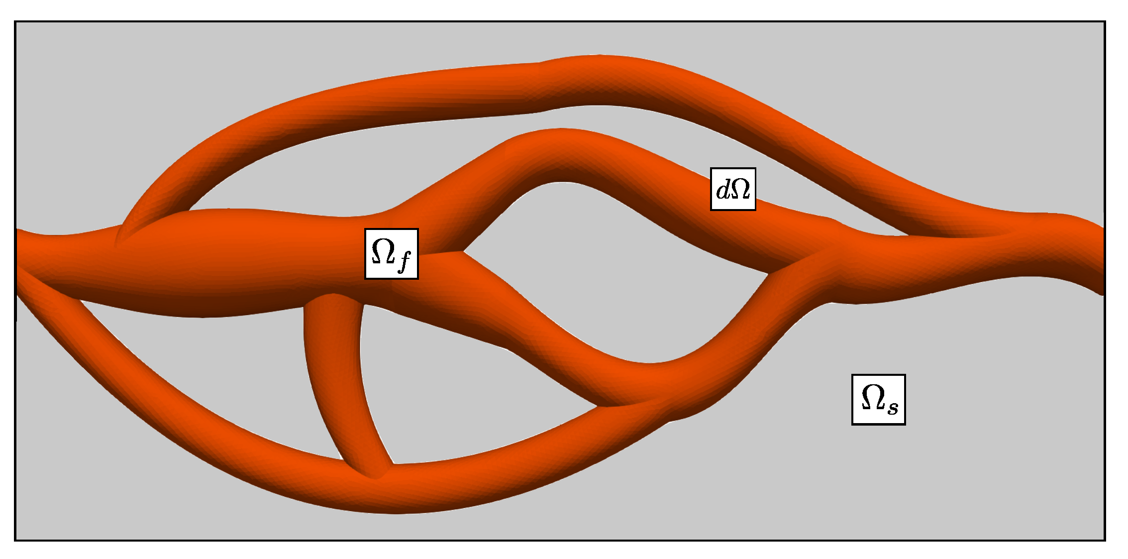
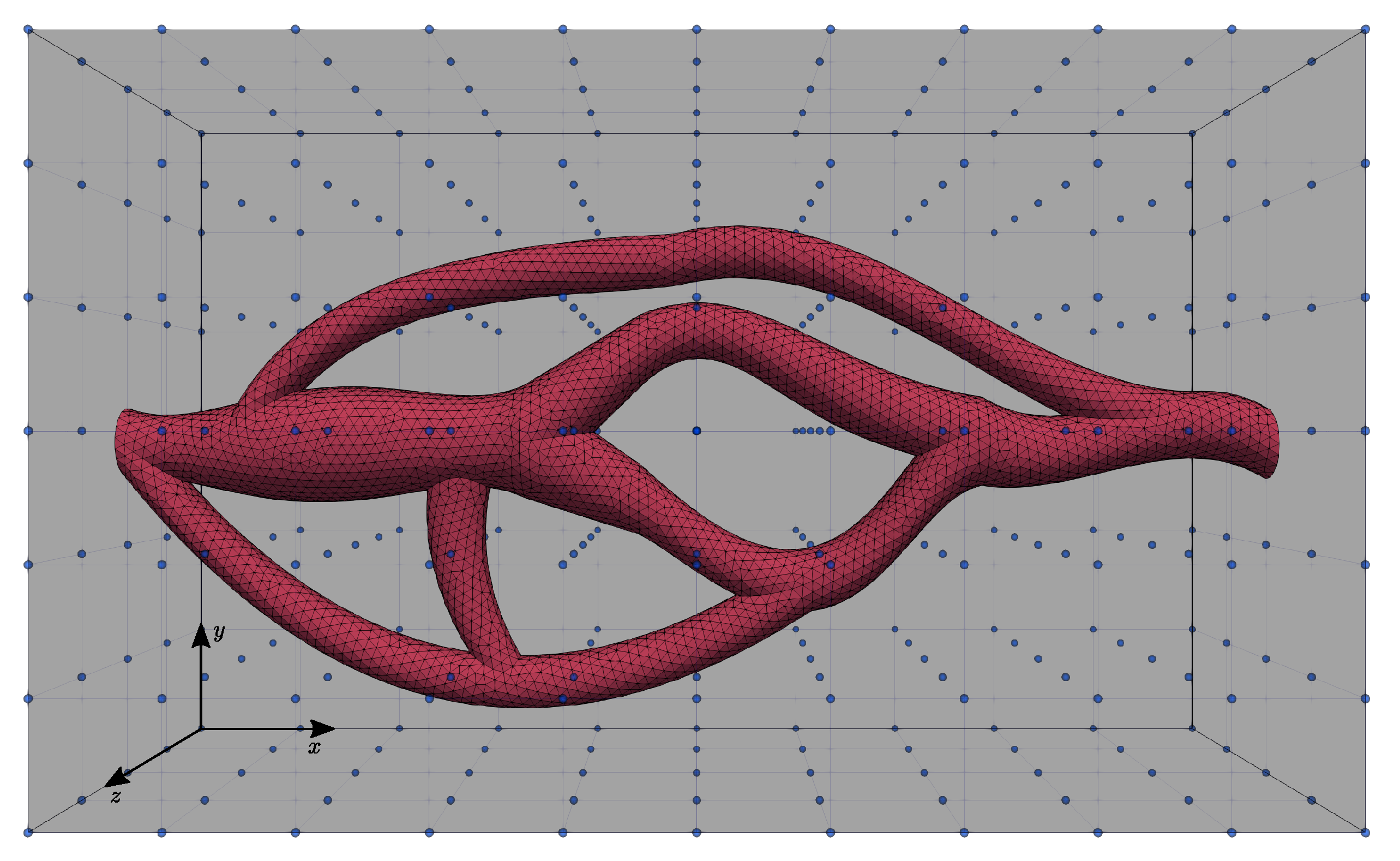
  • We first check the state of the computational grid node inside or outside the fluid domain ( Ω f ), defined by an Indicator function (I):
    I ( x ) = 1 x Ω f 0 x Ω s ,
    where x corresponds to the location of each computational grid node. We impose a rigid body motion to the nodes with I = 0 (e.g., u = 0 for a non-moving geometry) and the rest of the grid nodes (i.e., fluid grid nodes, I = 1 ) are considered for the flow computation.
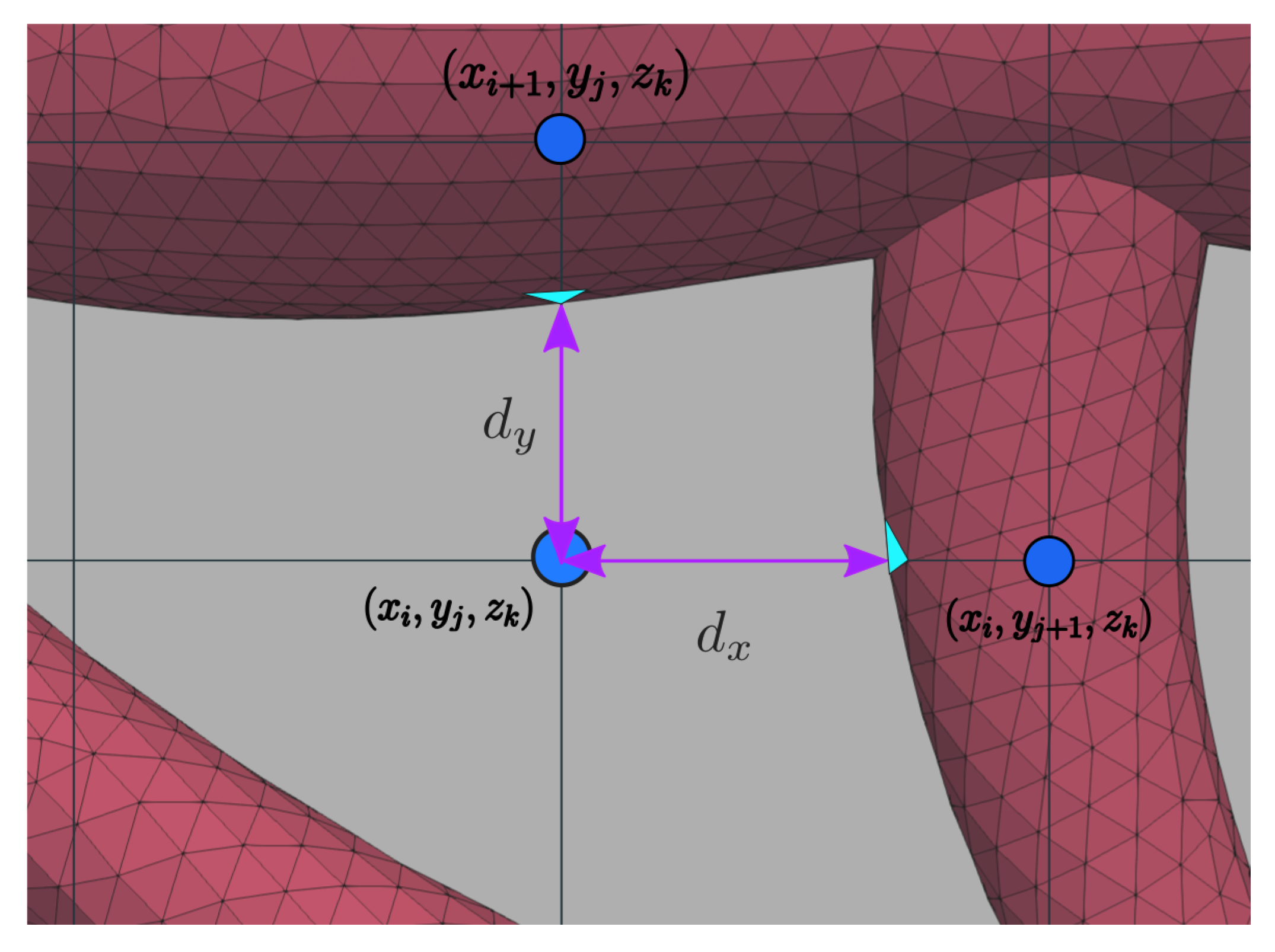
  • The presence of the interface is detected by the indicator function I. It is the location between two consecutive nodes where one node belongs to Ω f ( I = 1 ) and the other node belongs to Ω s ( I = 0 ), or vice versa. The accurate intersection distance of the neighbouring fluid node from d Ω is further estimated depending on the type of rigid body.
In case a rigid body shape is represented by an analytical expression such as a sphere, the intersection distance can be estimated numerically by defining a level set function for the rigid body. However, the process of finding the distances is more challenging for complex geometries defined by unstructured triangulated surfaces via STL files. In the next section, we provide the details of the strategy developed for complex geometries described by STL files.

3. Influence of Complex Geometries on Spatial Discretization

We extend the range of applications of the Direction Splitting method to complex geometries that can be described using an unstructured triangulated surface. The STL (Standard Triangle Language) format is widely used to represent triangulated surfaces. An STL file lists the vertices of the triangles defining the triangulation and their associated unit normal. In many fields involving flows in complex geometries, such as bio-fluid dynamics (e.g., blood flows [33]) or porous media (e.g., petroleum, geology [34]), an STL file describing the geometry is embedded into a flow solver.
The mapping of complex geometries by unstructured triangulations can be achieved in two ways: (1) using Computer-aided design (test cases Section 4.1, Section 4.2 and Section 4.4) with enough information describing the geometry. This usually guarantees a certain quality of generated triangulation, and (2) using imaging techniques such as CT scans and MRI (e.g., a complex network of blood vessels, CT scans of rocks; see test case Section 4.3). The volumetric image created by the stack of cross-sectional images represents the surface topology, which is discretized in the triangulation using algorithms such as Delaunay, frontal Delaunay or BAMG.
We now explain the methodology to consider the STL files in our Direction Splitting (DS) solver to perform flow in complex geometries. We achieve this by imposing a no-slip boundary condition on the triangulated surface. The framework of the present work relies on using a triangulation embedded in a uniform or non-uniform Cartesian grid. The domain inside and outside the triangulation corresponds to the fluid domain Ω f and the solid domain Ω s , respectively (see Figure 1). The surface of the complex geometry denoted d Ω behaves as a fluid-solid interface separating the grid nodes inside and outside the triangulation.
In order to explore flow configurations with an STL file, the numerical algorithm briefly presented in Section 2 requires the computation of indicator function (I) and intersection distances at each computational grid node. Unfortunately, STL geometries are a collection of triangulated surfaces, and the level set function cannot be easily defined. So, we calculate the intersection distance by resolving the intersection of a triangulated surface and a line connecting two grid nodes located on opposite sides of the triangulated surface. Figure 2 shows the considered STL with the computational grid nodes, the position of each node is defined with x ( i , j , k ) , where i, j and k are the indexes in each x, y and z direction, respectively.

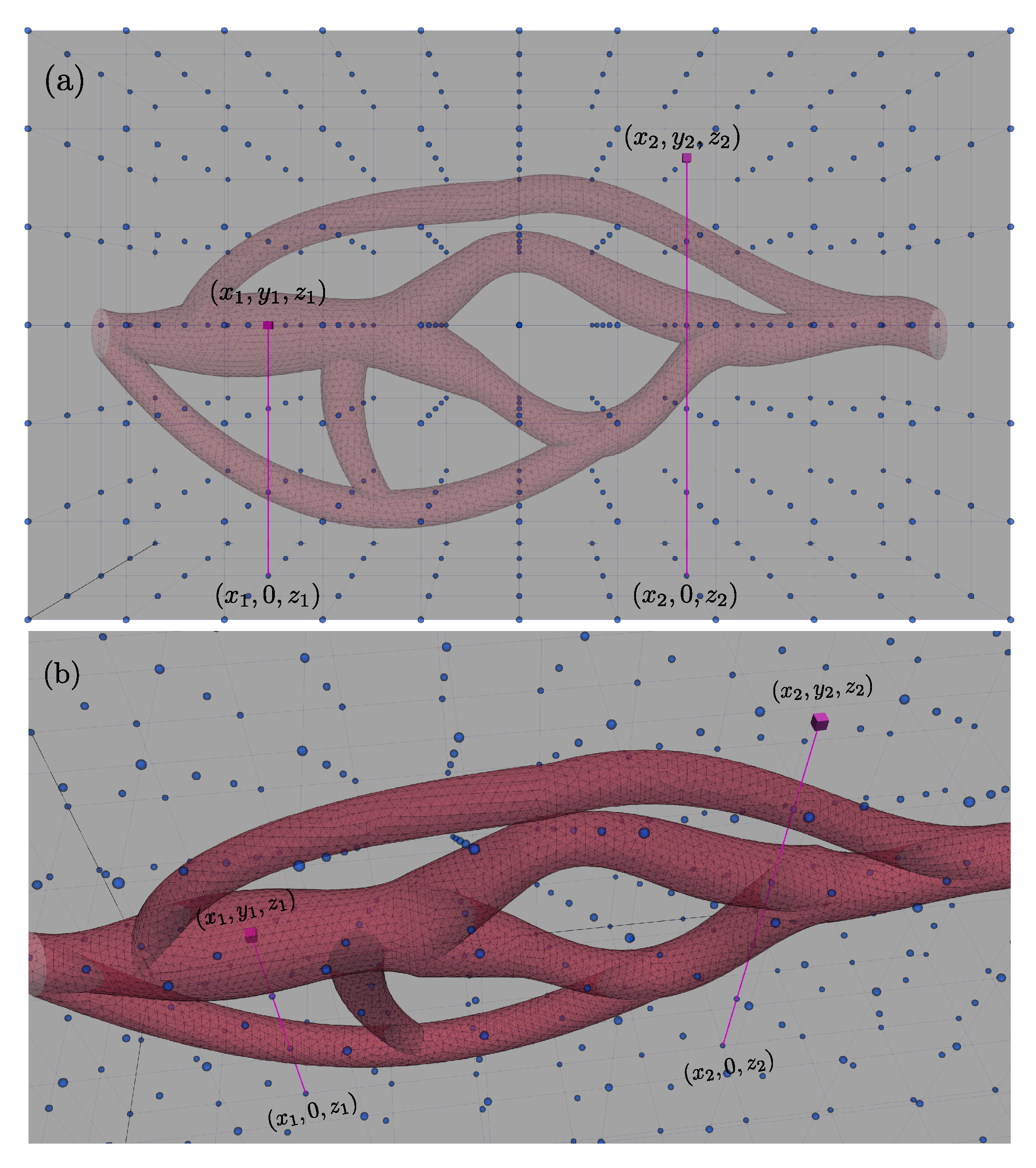
3.1. Indicator Function

We consider two grid nodes x 1 = ( x 1 , y 1 , z 1 ) and x 2 = ( x 2 , y 2 , z 2 ) as described in Figure 3; x 1 is located inside of the blood vessel ( x 1 Ω f ) whereas x 2 is located outside of the vessel ( x 2 Ω s ). The approach employed here is inspired by the ray-tracing techniques widely used in computer graphics. The ray is defined for each grid node as the segment connecting the node and its projection onto the x z plane. We then compute the number of intersections between the ray and the set of triangles contained in the STL file. Assuming that the geometry inlet and outlet are defined on two parallel planes orthogonal to the x axis, if the number of intersections is odd, the node belongs to the fluid domain, or to the solid domain otherwise. In Figure 3, the segment connecting x 1 and ( x 1 , 0 , z 1 ) intersects three times the triangulation, so I ( x 1 ) = 1 while the segment connecting x 2 and ( x 2 , 0 , z 2 ) intersects four times the triangulation and thus I ( x 2 ) = 0 . The sequence of instructions leading to the computation of I is listed in the Algorithm 1 below.
Algorithm 1 Computation of the indicator function (I) on a grid of size N x × N y × N z .
1:for i = 1: N x  do
2:    for j=1: N y  do
3:        for k = 1: N z  do
4:            x R 1 ( x ( i ) , y ( j ) , z ( k ) ) ▹ we build the two extremities of the ray
5:            x R 2 ( x ( i ) , 0 , z ( k ) )
6:           for sTdo▹ assuming T is the set containing the triangles
7:               if intersection(s, x R 1 , x R 2 ) then
8:                    n i n t n i n t + 1 ▹ number of intersections
9:               end if
10:           end for
11:           if  n i n t is even then
12:                I ( i , j , k ) 0
13:           else if  n i n t is odd then
14:                I ( i , j , k ) 1
15:           end if
16:            n i n t 0
17:        end for
18:    end for
19:end for

3.2. Fluid-Solid Interface Distances

We consider two neighbouring nodes along any direction: for example ( x i , y j , z k ) and ( x i , y j + 1 , z k ) or ( x i , y j , z k ) and ( x i + 1 , y j , z k ) as seen in Figure 4. The diffusion and divergence stencils have to be modified if the STL surface, i.e., the fluid-solid interface, is detected between two neighbouring nodes. We achieve this by computing the distance between the node located in the fluid domain and the intersection between a segment connecting the two nodes and the triangle located between the fluid and solid nodes. If the interface is located between two nodes aligned in the x,y or z direction, we denote that distance d x , d y or d z respectively (Figure 4). This approach ensures that the no-slip boundary condition is imposed at the interface.

3.3. Optimization of the Method

The computation of the indicator function and distances requires in terms of implementation to loop through the whole set of triangles to determine how many of them intersect a given ray (indicator function) or which triangle is located between a given pair of solid and fluid nodes (computation of distances). The computation of these geometric quantities is performed only once at a pre-step before the simulation as we assume that the rigid boundaries defined by STL files do not move, but the the associated computing time can be significant for very large triangulations (usually more than 10 5 triangles). Given the two following observations:
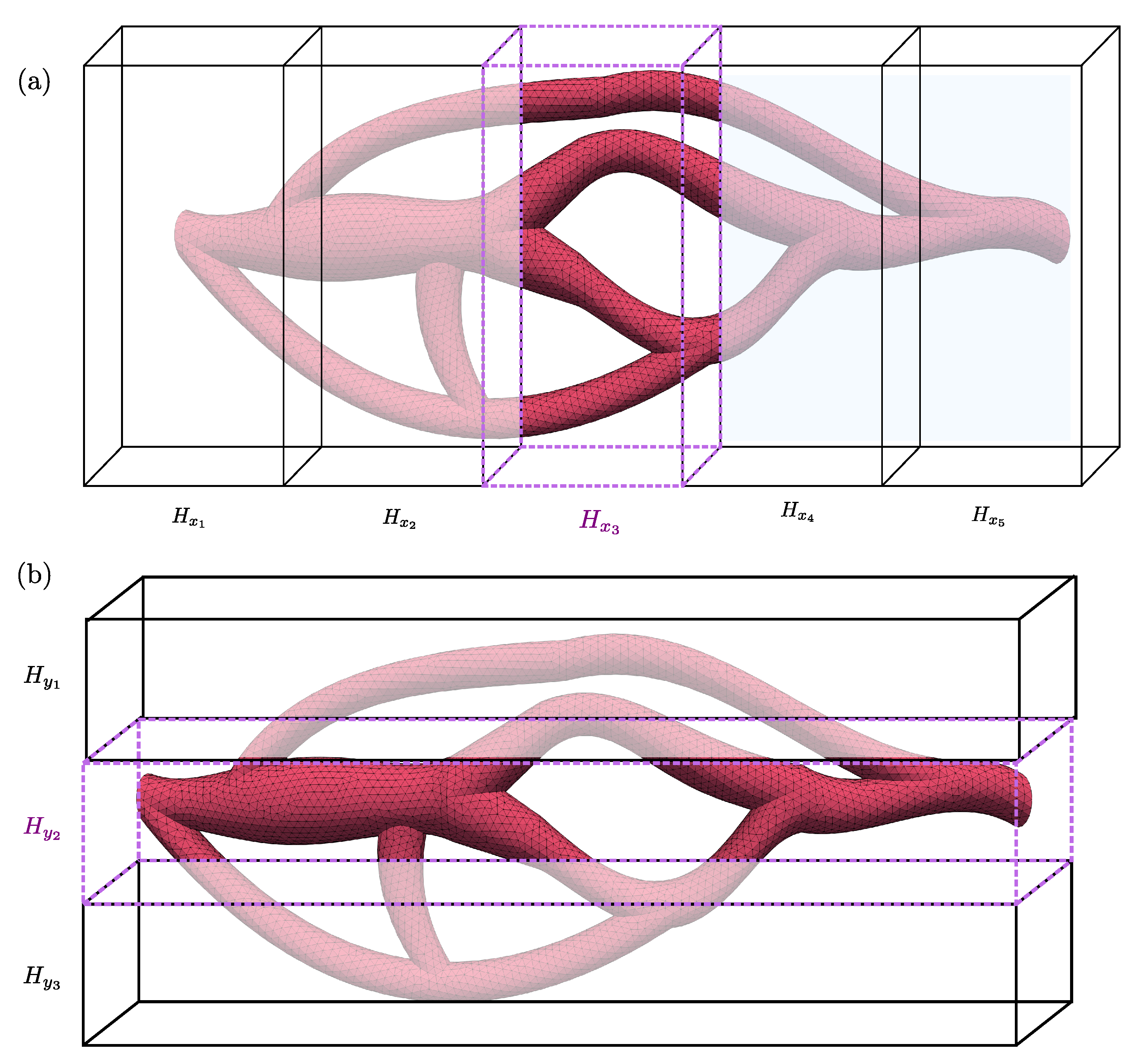
  • The rays used to compute the indicator function are by definition parallel to the y axis.
  • For a given pair of nodes, the node-triangle distance is computed along a line either parallel to the x, y or z axis.
We can reduce the list of triangles to loop through by introducing evenly sized subdivisions of the computational domain along the three directions. Each subdivision is an axis-aligned cuboid that contains a subset of the triangulation, as depicted in Figure 5. For the sake of simplicity, we sketched here subdivisions of the domain in two dimensions only. For a given node, the rectangles of interest are the ones located in the subdivision, along the y direction if we need to compute the indicator function, or along x,y or z if we need to compute a node-triangle distance. The size of the subdivision in each direction shall be chosen large enough such that no interference with the intersection function (ray-triangle) occurs.
This optimization is possible due to the formalism of the Direction Splitting method that does not rely on any 3 D distance computation which significantly decreases the computing time of the pre-step. In order to assess the efficiency of this optimization, we generate an STL file describing a sphere located at the center of a cubic computational domain. We carry out three simulations to measure the computing time of the pre-step. The three simulations correspond to three levels of STL refinement with 20 × 10 3 , 100 × 10 3 and 200 × 10 3 triangles respectively for small, medium and large triangulations. The wall time is measured for multiple realizations using a single computing core for a computational grid of 501 × 501 × 501 nodes. We subdivide the cubic computational domain into cuboids of equal size along each direction, N s is the number of subdivisions in each direction. Table 1 shows the wall time measurements for multiple combinations of N s and the number of triangles. The results clearly highlight the high efficiency of the optimization, reducing the wall time by a factor of 150, 36 and 17 for the small, medium and large triangulation, respectively.

4. Numerical Tests in Complex Geometries Described by STL Files

We consider flow configurations where the boundary of the flow domain is defined by triangulated surfaces. The simulations require the use of Cartesian grids, so the flow domain is embedded in a larger cuboid domain fully containing the triangulation. Surface triangulations used in Section 4.1 and Section 4.2 are generated and exported as STL files using the open-source meshing tool Gmsh [35]. The STL file used in Section 4.3 was downloaded from the digital Rocks portal: https://www.digitalrocksportal.org/projects/79/origin_data/312/ (accessed on 1 June 2022).

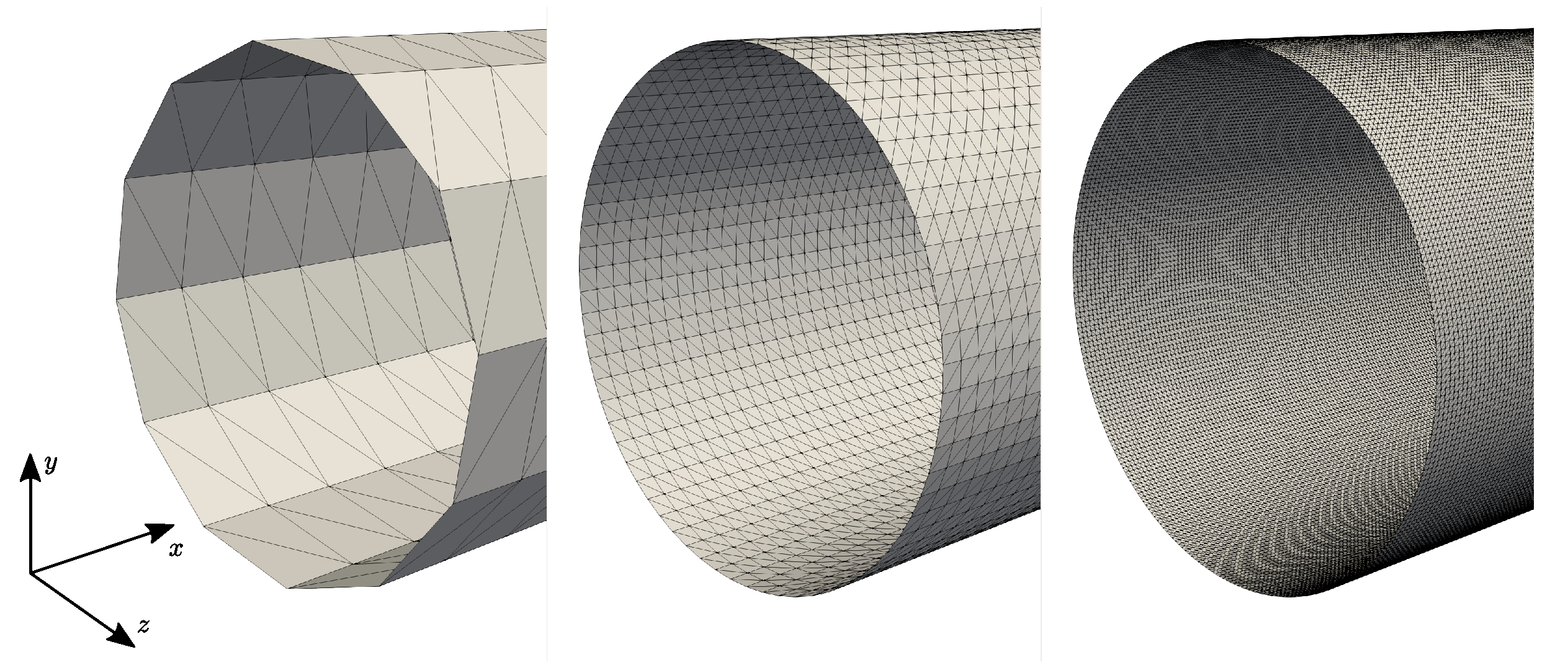
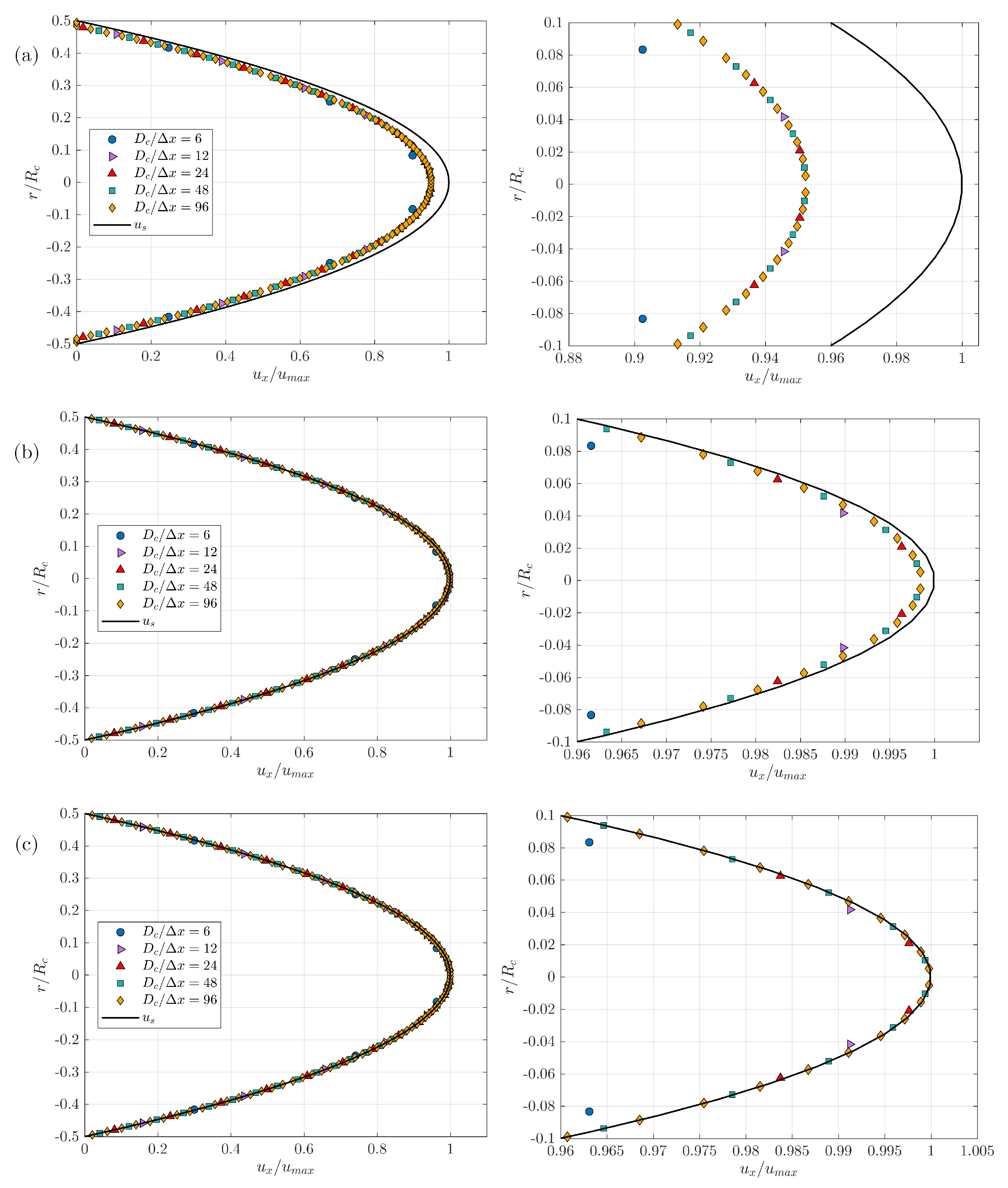
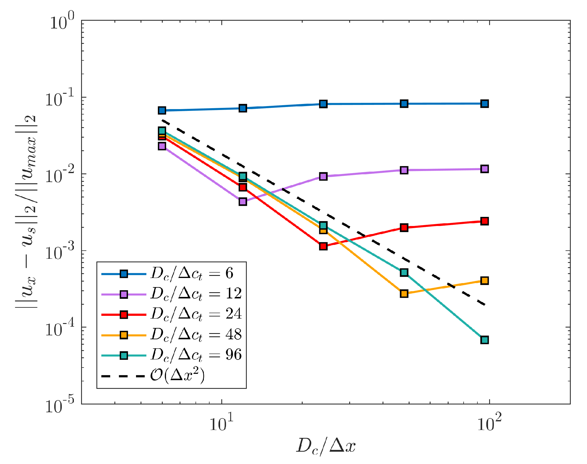
4.1. Poiseuille Flow in a Pipe

We place an axisymmetric cylinder of diameter D c = 2 R c = 1 and length L = 4 in a cuboid domain. Periodic boundary conditions are set at x = 0 and x = 4 . The flow is driven by an imposed constant pressure gradient. The associated Reynolds number based on the centerline velocity is R e = 2.5 . Arbitrary no-slip boundary conditions are set on the remaining faces of the cuboid.
We introduce the two parameters of interest for this test case: the number of grid nodes along the cylinder diameter D c / Δ x and the number of triangles along the cylinder diameter D c / Δ c t , with Δ c t the characteristic size of a given triangle defined as the length of the triangle smallest edge. D c / Δ c t describes the level of refinement of the STL file. As shown in Figure 6, the triangulation is built by mapping the surface of the cylinder with quadrilateral elements using a Delaunay algorithm; the triangulation is then simply obtained by dividing each quadrilateral element into two triangles of the same size. The mapping obtained is thus composed of triangles of the same size, resulting in a constant value of Δ c t across the triangulation. This allows us to directly investigate the influence of this parameter on the results: a potential disparity of the values of Δ c t across the triangulation may affect the simulation results but this analysis is not considered here. For all remaining test cases presented in this work, we always manage to generate a triangulation with relatively evenly sized triangles, so we can reasonably assume a unique value of Δ c t for the whole triangulation.
Simulations are run for D c / Δ x = { 6 , 12 , 24 , 48 , 96 } and D c / Δ c t = { 6 , 12 , 24 , 48 , 96 } . Figure 7 shows the streamwise component of the velocity u x scaled with the centerline velocity u m a x of the solution as a function of the radial distance r / R c , as well as the analytical solution u s of the Poiseuille flow in an axisymmetric pipe. Each plot corresponds to one value of the ratio D c / Δ c t = 6 , 24 or 96. As seen in Figure 6, for D c / Δ c t = 6 the STL triangulation barely describes the shape of an axisymmetric cylinder, therefore the computed profiles cannot be expected to converge towards the analytical solution u s . We however observe that the computed profiles show a converging behaviour. As the STL triangulation describes more and more accurately an axisymmetric cylinder, i.e., for increasing values of D c / Δ c t = 24 and 96, the profiles show really good agreement with the analytical solution u s . We can also highlight that a monotone behaviour for increasing values of D c / Δ x is observed for each plot. Finally, for all plots, while the relative difference of the profiles corresponding to D c / Δ x = 6 , 12 and 24 with respect to the analytical solution u s can be easily noticed, this difference is insignificant for D c / Δ x = 48 and 96.
We pursue the analysis by showing in Figure 8 on the same plot the velocity profiles for different ratios D c / Δ c t , where each plot corresponds to a given value of D c / Δ x ( 6 , 24 or 48) with increasing D c / Δ c t . The results show that for the smallest ratio D c / Δ x = 6 , a good agreement with the analytical solution u s can be achieved if the STL triangulation is well defined enough, for D c / Δ c t > 6 . Also, the relative difference with the analytical solution u s decays as D c / Δ c t increases and seems to be reaching a limit. This limits tends to be more and more shifted towards the analytical solution u s as D c / Δ x increases, as this limit quantifies how well the curvature of the axisymmetric cylinder is described. The agreement with the solution is increasingly better for D c / Δ x = 24 and D c / Δ x = 48 . The relative difference with the analytical solution u s is noticeable for D c / Δ c t = 6 across all plots, due to the fact that this ratio is critically low for the representation of the curvature of an axisymmetric cylinder. The results associated to D c / Δ x = 96 are not showed here but an excellent agreement with the solution is obtained, except for D c / Δ c t = 6 .
Figure 9 shows the combined influence of both ratios D c / Δ x and D c / Δ c t . The norm of the relative error scaled by the velocity of the analytical solution u s at the centerline | | u x u s | | 2 / | | u m a x | | 2 is reported as a function of D c / Δ x ; each line corresponds to simulations performed with the same STL file. Second order convergence is observed for all D c / Δ c t > 6 until Δ c t < Δ x . For Δ c t Δ x , the error slightly increases but stagnates, and remains of the same order of magnitude as the error corresponding to Δ x Δ c t . The optimal choice for Δ x and Δ c t is thus defined as Δ x Δ c t , or at least we shall ensure that Δ c t < Δ x . These final results determine the level of refinement of the STL files, since usually the ratio D c / Δ x is chosen beforehand.

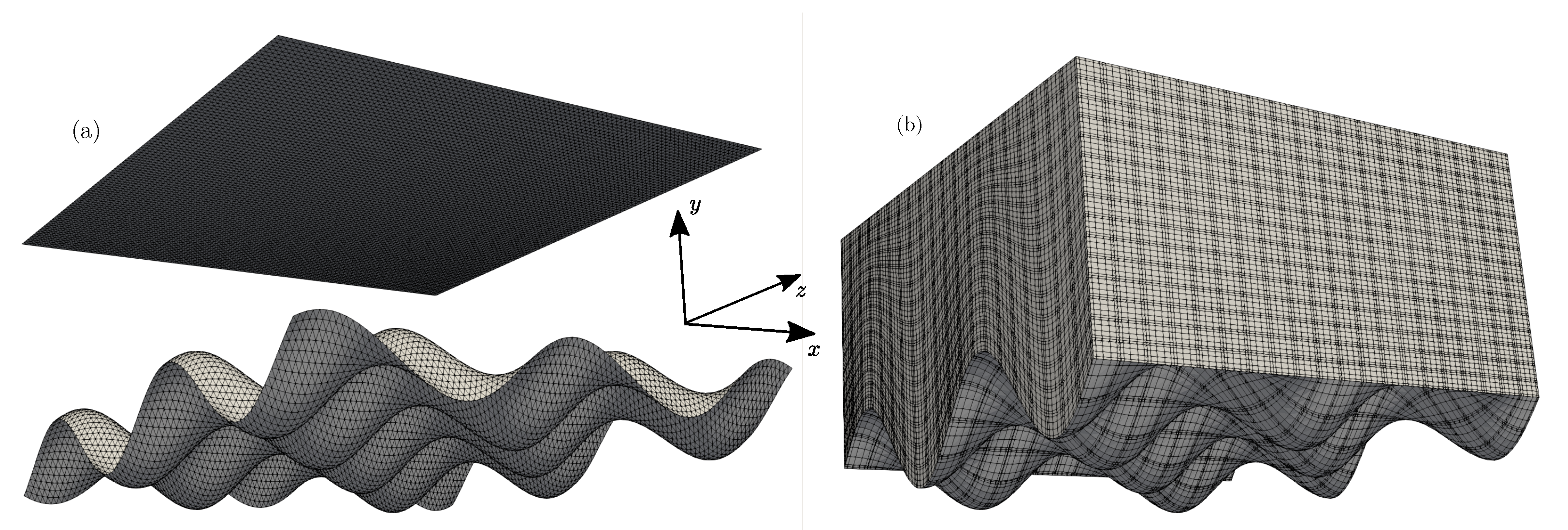
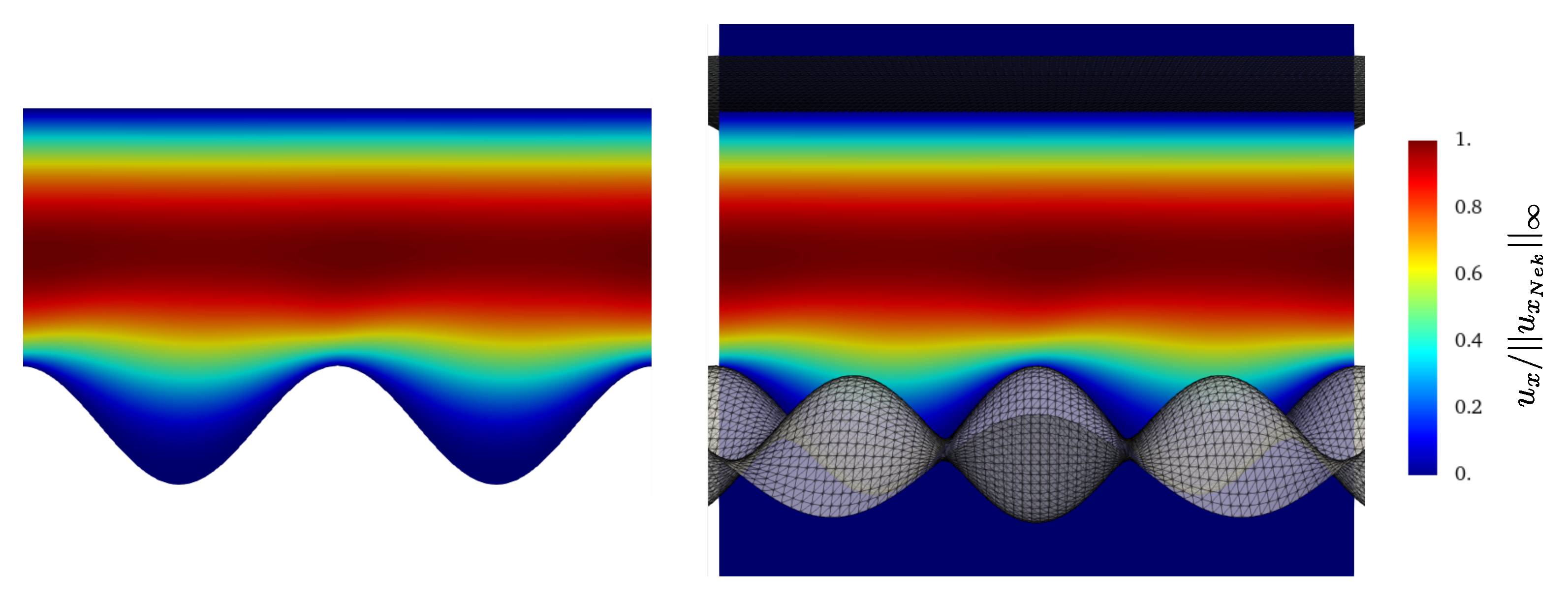
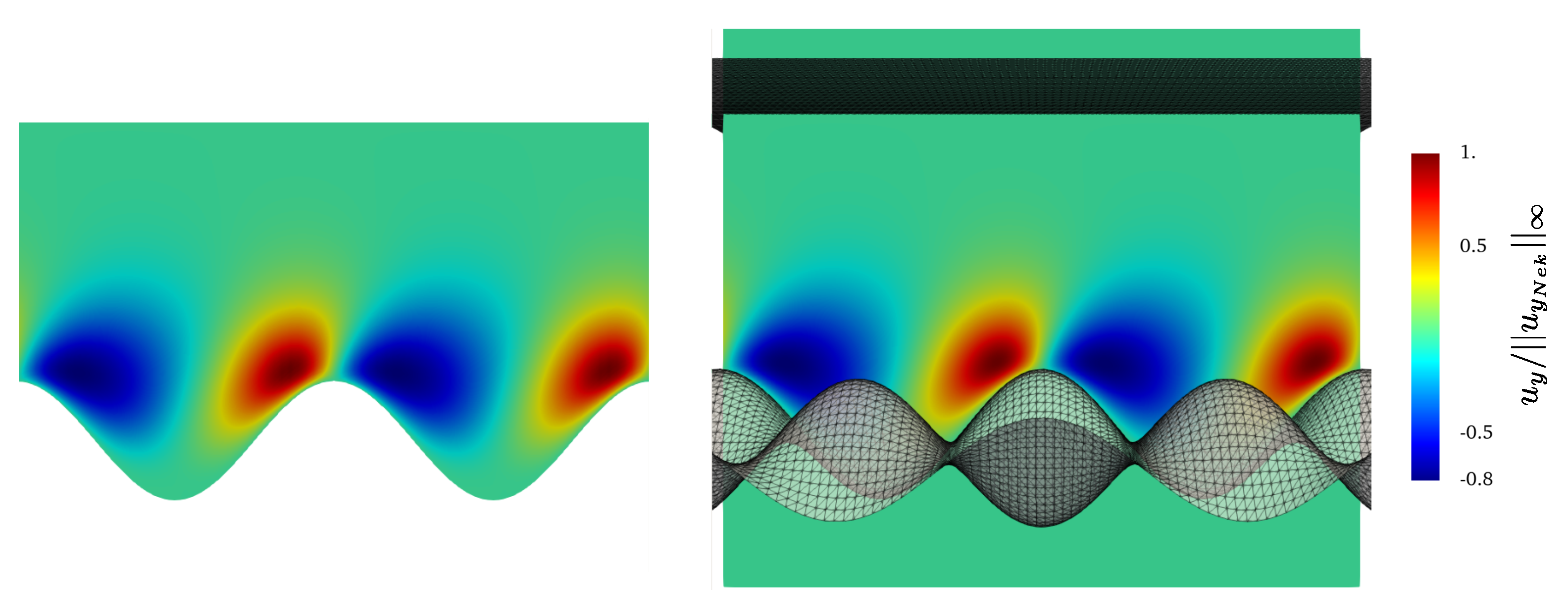
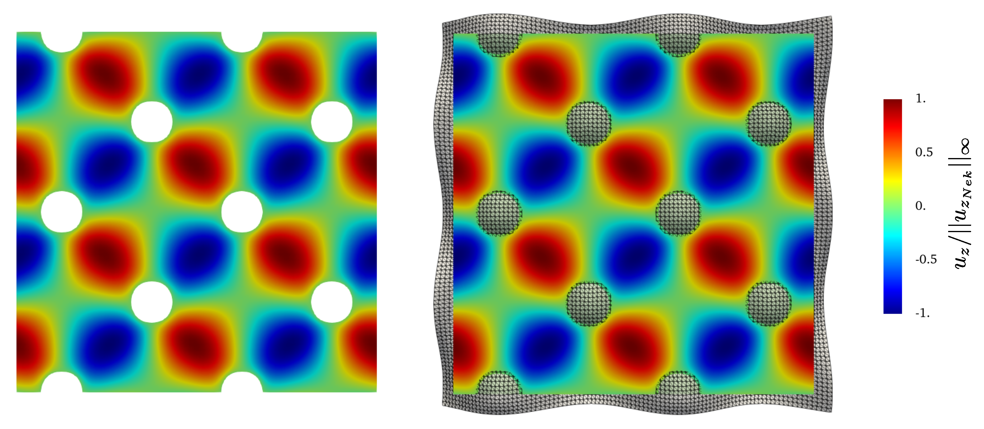
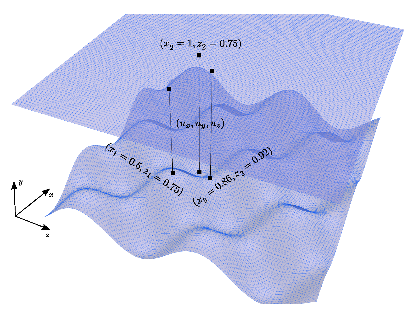
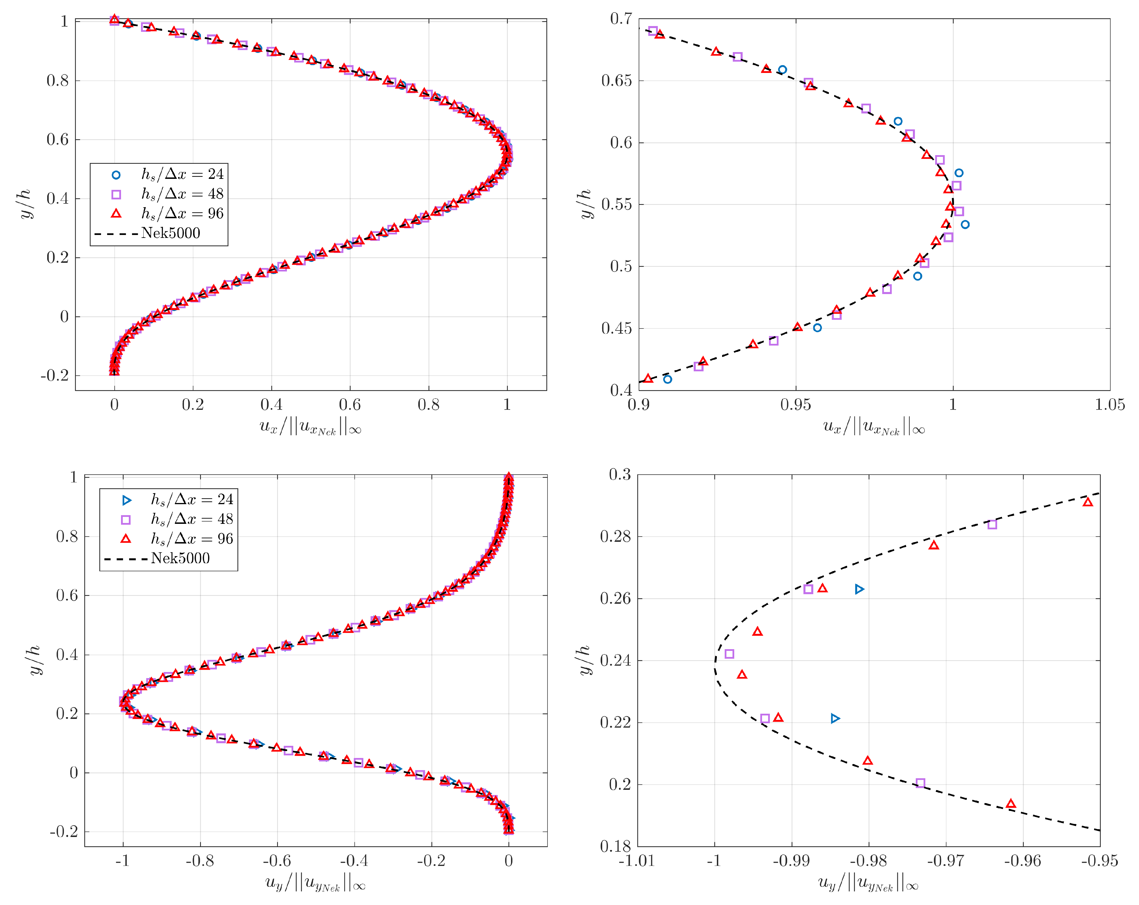
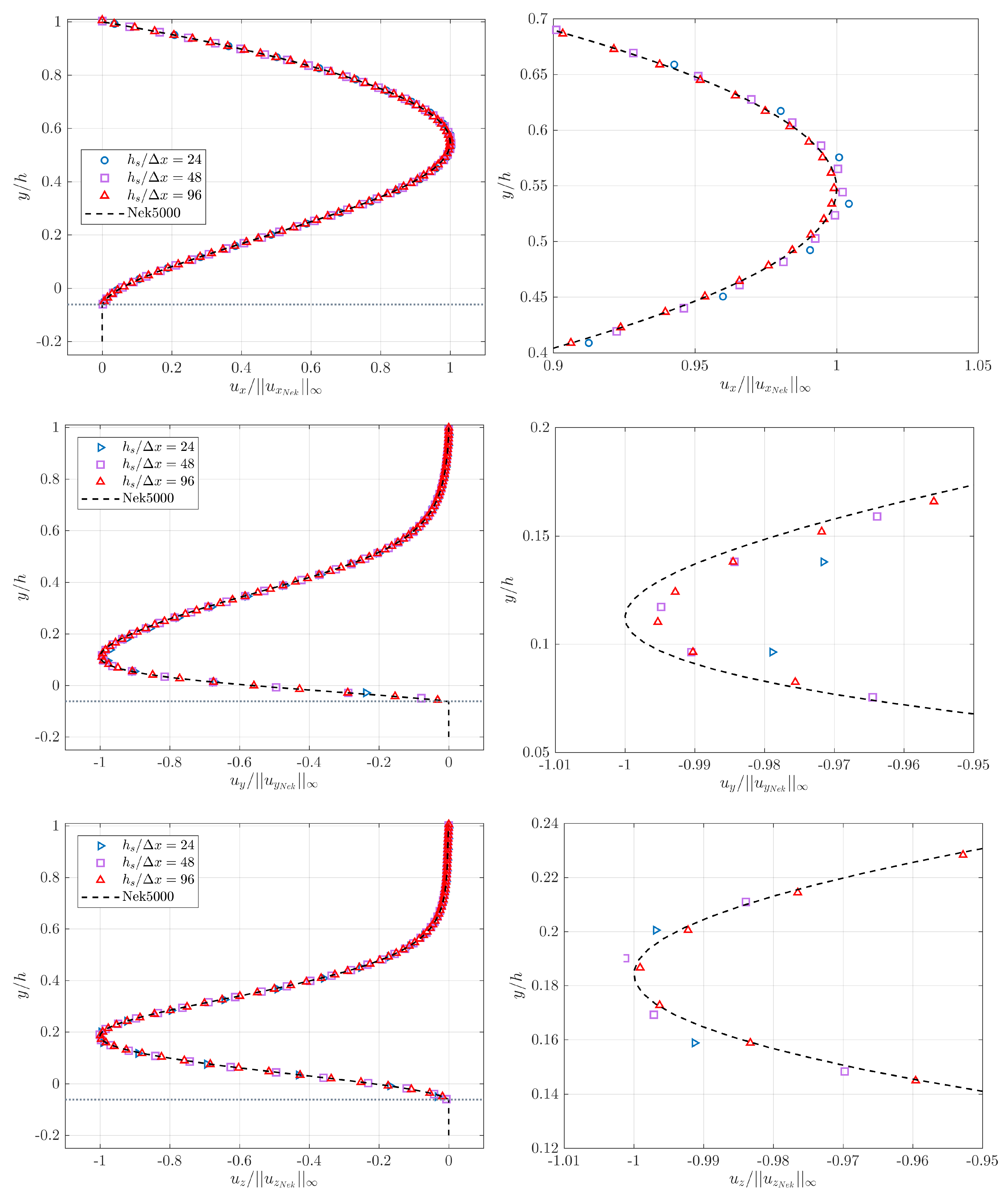
4.2. Flow in a Wavy Channel

We consider a flow in a bi-periodic channel in x and z directions (Figure 10). The top wall of the channel is a flat surface, while the bottom wall is a wavy surface parameterized by the function f ( x , z ) :
f ( x , z ) = A cos ( π x ) s i n ( π z )
We set the amplitude of the wave to A = 0.2 . We denote by h the average height of the channel, while h l and h s denote respectively the largest and smallest vertical amplitude of the channel bottom wall to top wall. We set the average height of the channel to h = 1 , thus h l = 1.2 and h s = 0.8 . The domain size is [ 0 , 2 ] × [ 0.2 , 1 ] × [ 0 , 2 ] and is embedded into a cuboid. Periodic boundary conditions are set at x = 0 and x = 2 , and at z = 0 and z = 2 . No-slip boundary conditions are applied at the bottom wavy wall and y = 1 . The flow is driven by an imposed constant pressure gradient. Assuming the pressure is normalized by p r e f = ρ f ( ν / h ) 2 , the normalized pressure gradient is set to d p d z h p r e f = 300 . We introduce a Reynolds number based on the fluid maximal velocity: R e m a x = ρ f | | u | | h / μ f = 31 . We set the time step magnitude such that the maximum CFL number is approximately 0.2.
The previous test case (Section 4.1) established the criteria ensuring a minimisation of the computational error due to the integration of STL files in the Direction Splitting method: the STL files used for this simulation are generated such that Δ c t < Δ x .
The purpose of this second test case is to compare the results provided by our solver with reference data provided by Nek5000 [36], an open-source spectral element code (SEM) developed at the Mathematics and Computer Science Division of Argonne National Laboratory. The spatial discretization is based on the spectral element method [37], which is a high-order weighted residual technique similar to the finite element method. SEM methods are well known for their accuracy, providing us with reliable reference data to compare our computed results to. The domain, initially a cuboid, is partitioned into E = 20 × 15 × 20 = 6000 hexahedral spectral elements of order N = 8 , which corresponds to the number of Gauss-Legendre-Lobatto (GLL) points per element along each direction. We use a feature of Nek5000 that allows the modification of the mesh (initially a cuboid) given some parametrization f ( x , z ) . The modification is applied to the GLL points directly; the modified mesh based on f is shown in Figure 10b. The simulation is run with Nek5000 until a steady state is reached, with a maximum CFL of 0.1.
We perform three simulations with the Direction splitting solver, corresponding to h s / Δ x = 24 , 48 and 96, and waited for the results to converge to a steady state. We show in Figure 11, Figure 12, Figure 13 and Figure 14 snapshots of respectively u x and u y in a plane orthogonal to the z axis located at z = 1.19 , and u x and u z in a plane orthogonal to the y axis located at y = 0.15 . u x is scaled by the infinite norm across the plane of the x component of the reference solution velocity | | u x N e k | | , u y is similarly scaled by | | u y N e k | | and u z is similarly scaled by | | u z N e k | | . The snapshots compare the results provided by the Direction Splitting method with the reference data (Nek5000). The results show excellent agreement with the reference data.
We also compare velocity profiles for u x , u y , u z along the lines intersecting the top wall orthogonally and the points ( x 1 = 0.5 , z 1 = 0.75 ) , ( x 2 = 1.0 , z 2 = 0.75 ) and ( x 3 = 0.86 , z 3 = 0.92 ) (see Figure 15). ( x 1 , z 1 ) and ( x 2 , z 2 ) are chosen because they are located respectively on the highest and lowest amplitude of the bottom wall, i.e., f ( x 1 , z 1 ) = 0.2 and f ( x 2 , z 2 ) = 0.2 . u z = 0 at these locations so we select ( x 3 , y 3 ) to be able to have a comparison for the third component of the velocity.
Figure 16 and Figure 17 show the components u x and u y of the velocity measured along the line intersecting ( x 1 , z 1 ) and ( x 2 , z 2 ) respectively for each h s / Δ x = 24 , 48 and 96 and the solution provided by Nek. u x is scaled by the infinite norm of the x component of the reference solution velocity | | u x N e k | | along each line, u y is similarly scaled by | | u y N e k | | . Results in both figures show a converging trend with increasing h s / Δ x and very satisfactory agreement with the reference data for u x with a relative error less than 1%. Same observations can be made for u y although the error is slightly higher, which is due to the fact that we used linear interpolation to compute the velocity profiles, ( x 1 , z 1 ) and ( x 2 , z 2 ) do not necessarily coincide with the grid nodes. Same comment applies to the reference data, ( x 1 , z 1 ) and ( x 2 , z 2 ) are not necessarily located on the GLL points either. The u y velocity profile exhibit sharper spatial variations than the u x velocity profile, especially in the vicinity of its maximum value. We explored other methods of interpolation, but the linear interpolation provided the best results. u z is not shown here since its value is zero along the two profiles associated to ( x 1 , z 1 ) and ( x 2 , z 2 ) due to the flow symmetry across the bumps in the z direction. The values of u z are reported to be less than 10 6 for both profiles and for each h s / Δ x .
Figure 18 shows the same analysis with a non-trivial u z in addition, scaled by | | u z N e k | | . Again, the agreement with the reference solution is excellent and a converging trend with increasing h s / Δ x is observed for each component. Concerning the slightly higher relative error we observe for u y , the same observation regarding the use of linear interpolation can be made.

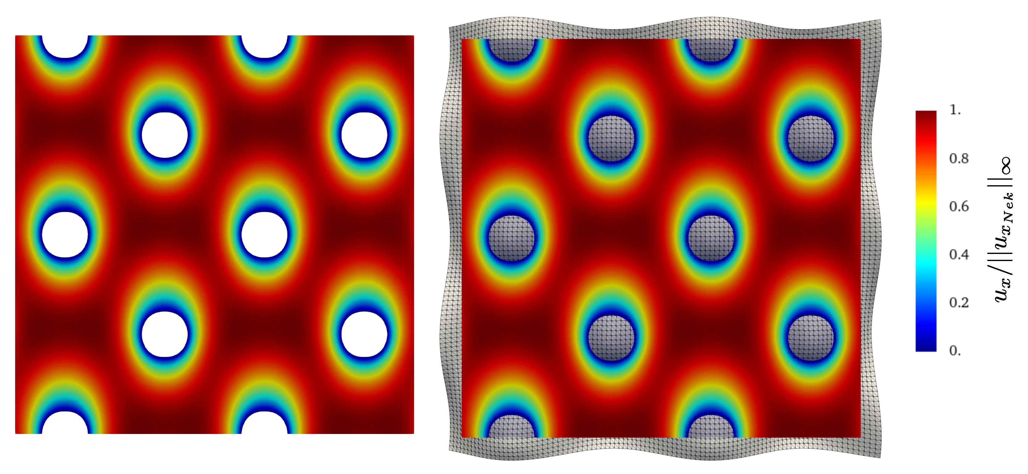
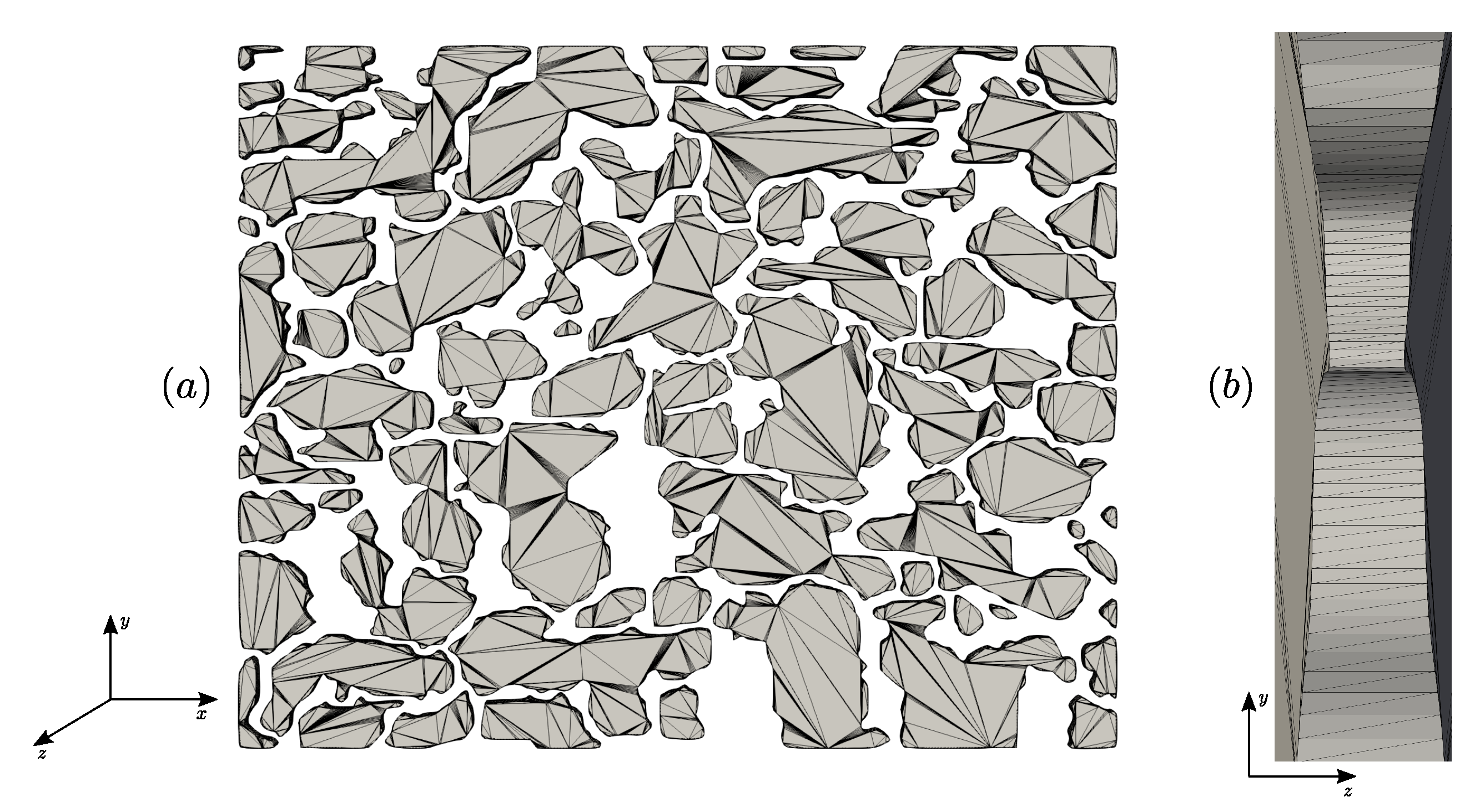
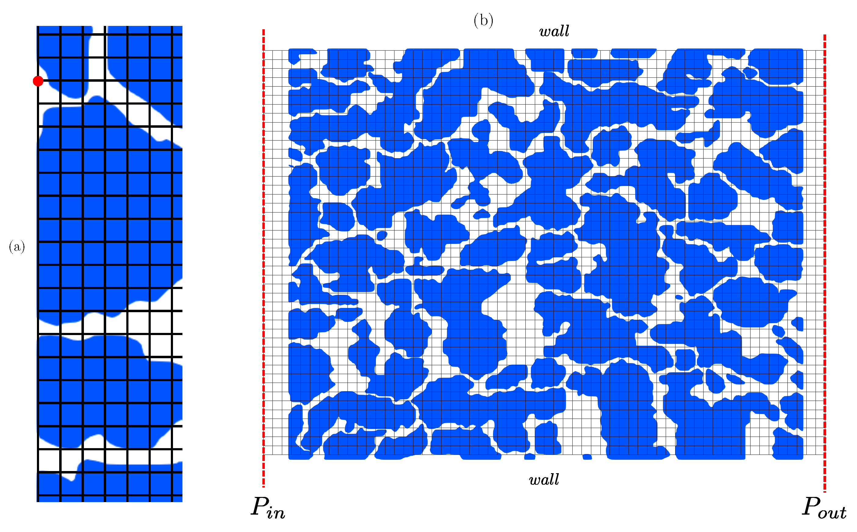
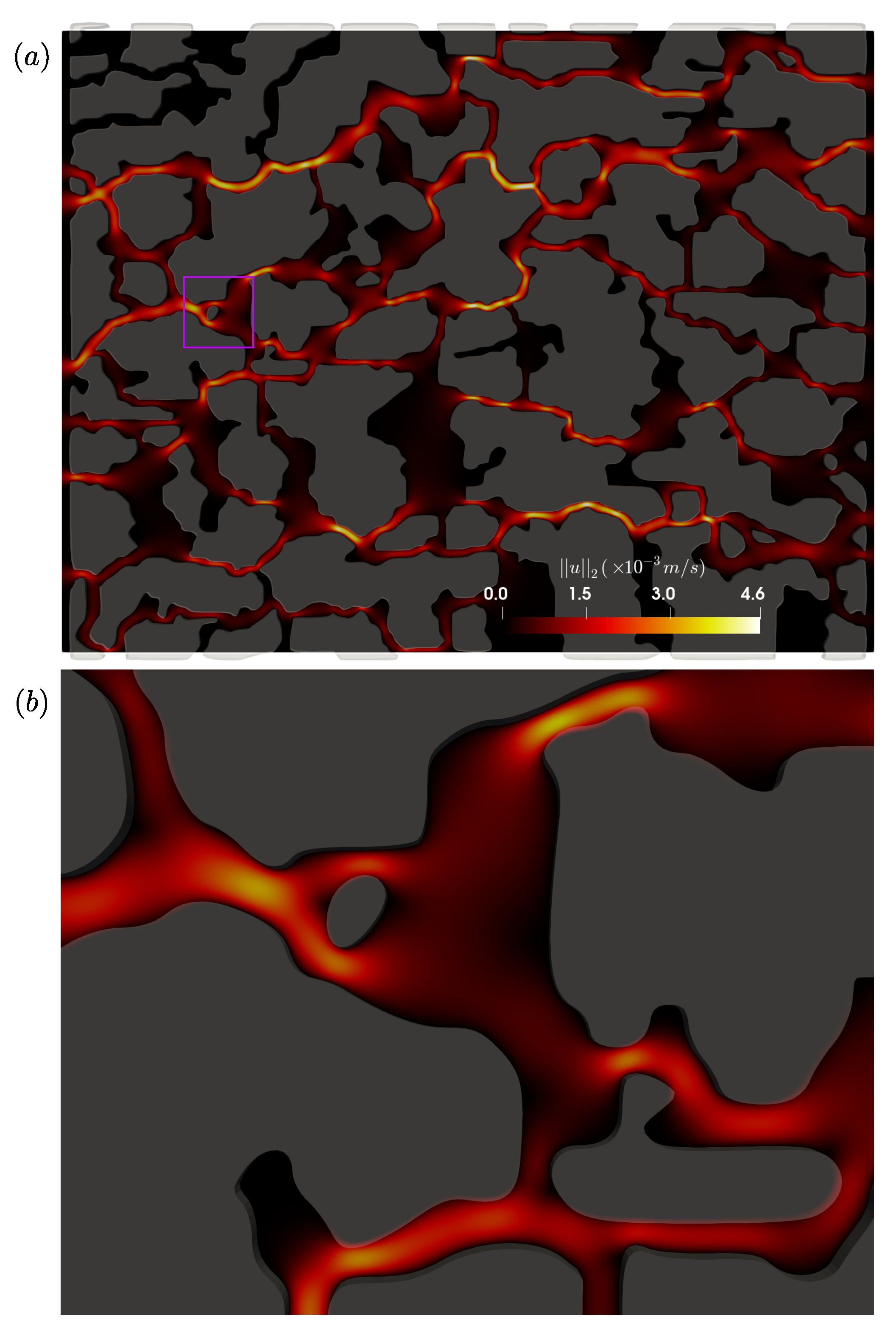
4.3. Flow in a Porous Medium: Computation of the Permeability Coefficient in a Sandstone

We study the flow in a sandstone whose structure describes a porous medium. Performing flow simulations in porous materials such as rocks or similar media is relevant to many applications, such as oil recovery processes, soil infiltration, or pollutant leakage in geological strata. The permeability of a material describes how much it resists the flow of fluids. In oil-related industrial applications, an accurate measure of permeability is key because the greater the permeability, the easier it is to extract oil from the rock.
The objective of this test case is to compute the permeability coefficient of a sandstone medium. Darcy’s law describes the motion of a fluid through porous media: it states that the flow rate is linearly proportional to the force driving the fluid. Darcy’s law can be written as:
Q = k A ( P o u t P i n ) μ f L
with Q the volumetric flow rate (m3/s), k the permeability of the porous medium (m2), A the cross-sectional area m2, ( P o u t P i n ) the pressure drop across the medium (Pa), μ f the fluid viscosity (Pa·s) and L the domain length (m). The permeability coefficient is obtained by setting a pressure drop and measuring the induced volumetric flow rate.
Figure 18. Profiles of u x , u y and u z for h / Δ x = 24 , 48 , 96 along the wall-normal direction, profile set at ( x 3 , z 3 ) .
Fluids 08 00086 g018
The computational domain is a planar 3D micromodel: the STL file is built by adding thickness to a 2D image in the z direction as shown in Figure 19. The domain occupied by the sandstone is [ 0 , 1774 ] × [ 0 , 1418 ] × [ 12.27 , 12.27 ] μm3. We simplify the STL file provided by [34] by consequently reducing its size: we only need to ensure that the criteria established in Section 4.1 Δ c t < Δ x is satisfied, there is no requirement to choose Δ c t very small compared to Δ x . Given our framework the initial triangulation was unnecessarily highly refined, leading to a high computing time for the pre-step at which the indicator function is computed. Figure 19 shows the STL triangulation used for the simulations, and we can observe that the triangles are relatively large on the front and back faces orthogonal to the z axis (Figure 19a) which is of no importance since there are located on a planar surface. The triangles mapping the pores of the sandstone are evenly sized (Figure 19b) and verify for all simulations Δ c t < Δ x .
Using the same approach as that employed in [34], we embed the triangulation in a cuboid domain but we append a buffer region to the inlet and outlet of the domain and shorten the boundaries in the y direction by a thin layer, which makes the implementation of boundary condition easier as shown in Figure 20. Without a buffer region, it would have been required to provide an approach detailing how to write certain boundary conditions (like a pressure drop) when the nodes located on the inlet and outlet boundaries belong either to the fluid domain or to the solid domain (see Figure 20). Removing a thin layer in the y direction allows to avoid edge effects of the STL triangulation. The buffer size is 2% of the x length of the domain, the thin layer size represents 2% as well of the y length of the domain. The size of the layers has been investigated and no influence on the results is observed.
We impose a pressure drop along the x direction of the domain: ( P o u t P i n ) = 100 Pa. Periodic boundary conditions are set in the z direction and wall boundary conditions are set on the remaining faces of the cuboid. We define the Reynolds number as R e = ρ f u d h / μ f , with u d the Darcy velocity (flowrate divided by the inlet/outlet area), and h the thickness of the domain in the z direction. We set μ f = 10 3 Pa·s and ρ f =1000 kg·m−3. The corresponding Reynolds number is R e = 0.002 .
We perform simulations on 3 different grids: N x × N y × N z = 720 × 560 × 2 , 1440 × 1120 × 2 and 2880 × 2240 × 2 . Two nodes only are required along the z periodic direction of the domain. In order to study the influence of the time step magnitude on the permeability measurement, we use three different time steps: Δ t = 10 6 s, Δ t / 2 and Δ t / 4 . The maximum CFL number is approximately 0.2. Once the steady state is reached (Figure 21), we compute the permeability coefficient k. Figure 22 shows the permeability coefficient as a function of N x , for Δ t = 10 6 s, Δ t / 2 and Δ t / 4 . Very satisfactory agreement with the permeability coefficient value reported by the DNS simulations of [34] is observed. Reducing the time step magnitude for the runs corresponding to the grid N x × N y × N z = 720 × 560 × 2 did not improve the permeability measurement. This is due to the fact that for this grid refinement, the smallest gaps of the domain are only meshed across 8 grid nodes, thus spatially underesolving the fluid flow. For the two remaining grids, we observe that reducing the time step magnitude decreases the relative error. Overall increasing N x improves the agreement with the value of k reported by [34].

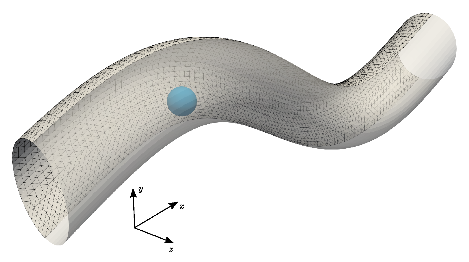
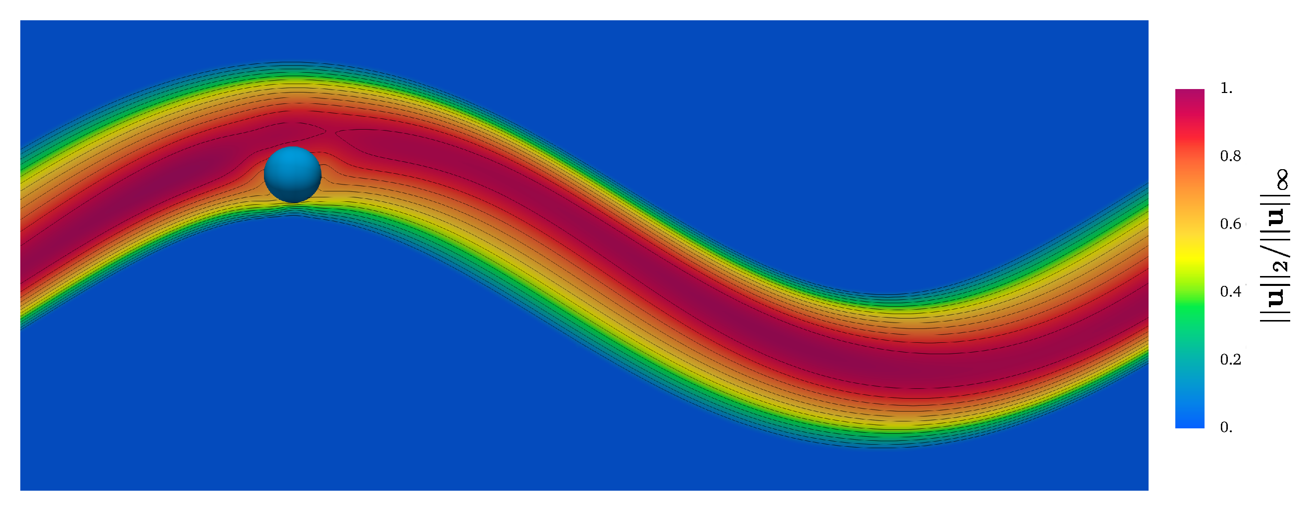
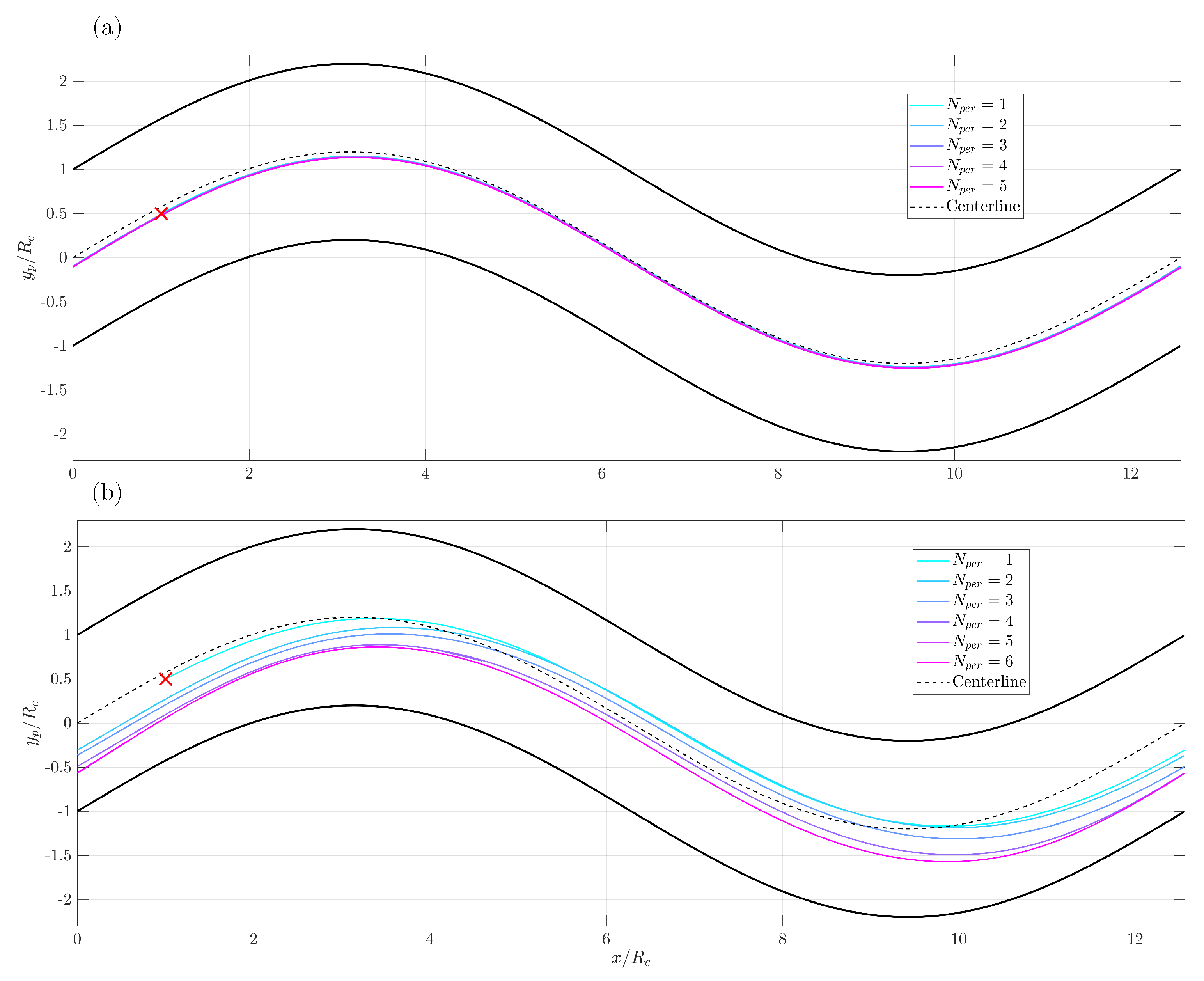
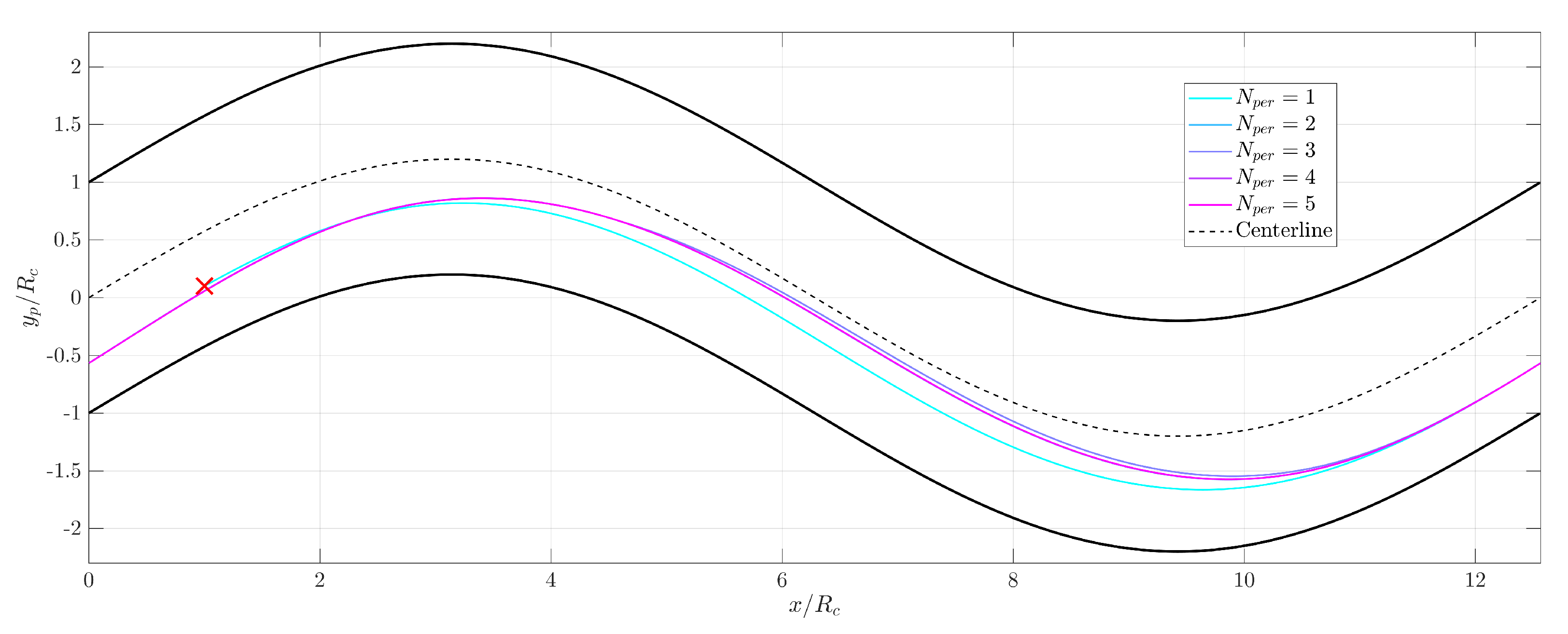
4.4. Motion of a Rigid Spherical Particle in a Curved Pipe

This test includes the motion of a spherical particle in a fixed pipe (Figure 23). The motion of the sphere is governed by the equation of motion (Equation (2)) combined to a kinematic equation for the time evolution of the position of the center of mass of the sphere, i.e., the trajectory of the sphere. Since the sphere never collides with the pipe wall, we do not need to use any particle-wall collision model. Consequently, the force F and the torque T in Equation (2) simply correspond to the hydrodynamic force and torque, respectively. We also assume that the sphere is neutrally buoyant, i.e., ρ s = ρ f , and we denote its radius R p , therefore the complete set of equations of the sphere motion is:
ρ s 4 3 π R p 3 d U d t = F = d Ω s ( p I + μ f ( u + u t ) ) · n d S , ρ s 8 15 π R p 5 d ω d t = T = d Ω s R p n × ( p I + μ f ( u + u t ) ) · n d S , d X d t = U ,
where d Ω s denotes the sphere surface, d S the elementary surface area, n the outwards oriented unit normal vector to the sphere surface, . t the transposed operator, I the identity matrix and X the position of the center of mass of the sphere. F and T are computed by accurate numerical integration of the fluid stress tensor on the sphere surface. For the purpose of numerical integration, the sphere surface is discretized in a set of non-overlapping rectangles of approximately same surface area and a 2D mid-point rule is applied in each rectangle, leading to second order spatial accuracy. We use the method of level set and triangular intersections for sphere and STL, respectively, for I and intersection distance calculations to showcase the applicability of the DS solver in a complex flow configuration with STL geometries (here the curved pipe) and simple particle shapes (here the sphere).
The cross-section of the pipe is a disk of radius R c = 1 . The y position of the centerline of the pipe is parameterized by g ( x ) = A sin ( x / 2 ) with A = 1.2 R c = 1.2 . The pipe is embedded into a cuboid computational domain of size [ 0 , 4 π R c ] × [ 2.5 R c , 2.5 R c ] × [ 1.5 R c , 1.5 R c ] . Periodic boundary conditions are set at the inlet and outlet of the curved pipe; wall boundary conditions are set elsewhere. We set R p = 0.3 and initially locate the sphere at ( x p / R c , y p / R c , z p / R c ) = ( 1 , 0.5 , 0 ) , slightly below the centerline. The flow is driven by an imposed constant pressure gradient and the particle is released at rest at t = 0 . We carry out two simulations corresponding to two fluid Reynolds numbers (based on the fluid maximal velocity R e = ρ f | | u | | 2 R c / μ f ) of R e = 12 and R e = 115 . The associated particle Reynolds numbers based on the particle maximal velocities R e p = ρ f | | u p | | 2 R p / μ f are respectively R e p = 3 and R e p = 30 . The maximum | | u | | and | | u p | | are computed over all time iterations. The ratio of grid nodes per diameter is set such that 2 R c / Δ x = 24 . The time step magnitude is set such that the maximum CFL is 0.25. We also test for the same flow conditions a different initial position for the particle ( x p / R c , y p / R c , z p / R c ) = ( 1 , 0.1 , 0 ) , i.e., more shifted below the centerline, for the case corresponding to R e = 113 . The values of the maximum fluid and particle Reynolds numbers remain close for both initial positions of the particle, the slight difference (113 compared to 115) is only due to the transient flow and transient trajectory that depend on the particle initial position.
A snapshot of the flow field is shown in Figure 24. In the absence of buoyancy, the motion of the particle is entirely governed by the hydrodynamic force and torque exerted by the fluid flow on the particle. The flow carries the particle, and thus the particle relative velocity with respect to the fluid is relatively low. This causes a limited footprint of the particle on the flow, as seen in Figure 24.
We report in Figure 25 the y component of the particle position as a function of x in the x y plane, both scaled with the pipe radius R c . No particle motion across the z axis was observed. The pipe is periodic and the particle is relocated at the entrance of the domain after completing a whole period. Each period is labelled separately as shown in Figure 25; e.g., N r e p = 3 corresponds to the third crossing in the fluid domain. We observe that for the lowest Reynolds number R e = 12 , even if the particle position is slightly shifted off the centerline, we can reasonably affirm that the particle follows the center streamline. Across all periods, the trajectories are identical. Inertial effects play a larger role for R e = 115 : the particle center intersects multiple times the centerline before finally settling in the lower part of the pipe and moving along the same path, with the plots corresponding to N r e p = 5 and 6 overlapping perfectly.
We shifted the particle in the y direction towards the lower part of the pipe for the case corresponding to R e = 113 . We can observe that for this initial position the particle center does not intersect the centerline (Figure 26). After the first period, the particle repeatedly moves along the same path in the channel. These observations highlight the strong influence of the particle initial position over the transient of the particle trajectory, potentially preventing it from any cross-centerline migration. Please note that the steady-state trajectory of the particle in the pipe is independent of its initial position, as expected. Indeed, trajectory N p e r = 6 in Figure 25b is similar to trajectory N p e r = 6 in Figure 26. While a thorough analysis of the particle trajectory is beyond the scope of the present paper, we postulate that the off-centered trajectory of the particle in the inertial case R e = O ( 100 ) is the result of the Segre-Silberberg effect [38] combined to the curvature of the pipe. Investigating the migration potential of a set of particles is key in numerous fields of application, especially in microfluidics, a field in which we intend to use the method presented in this work.

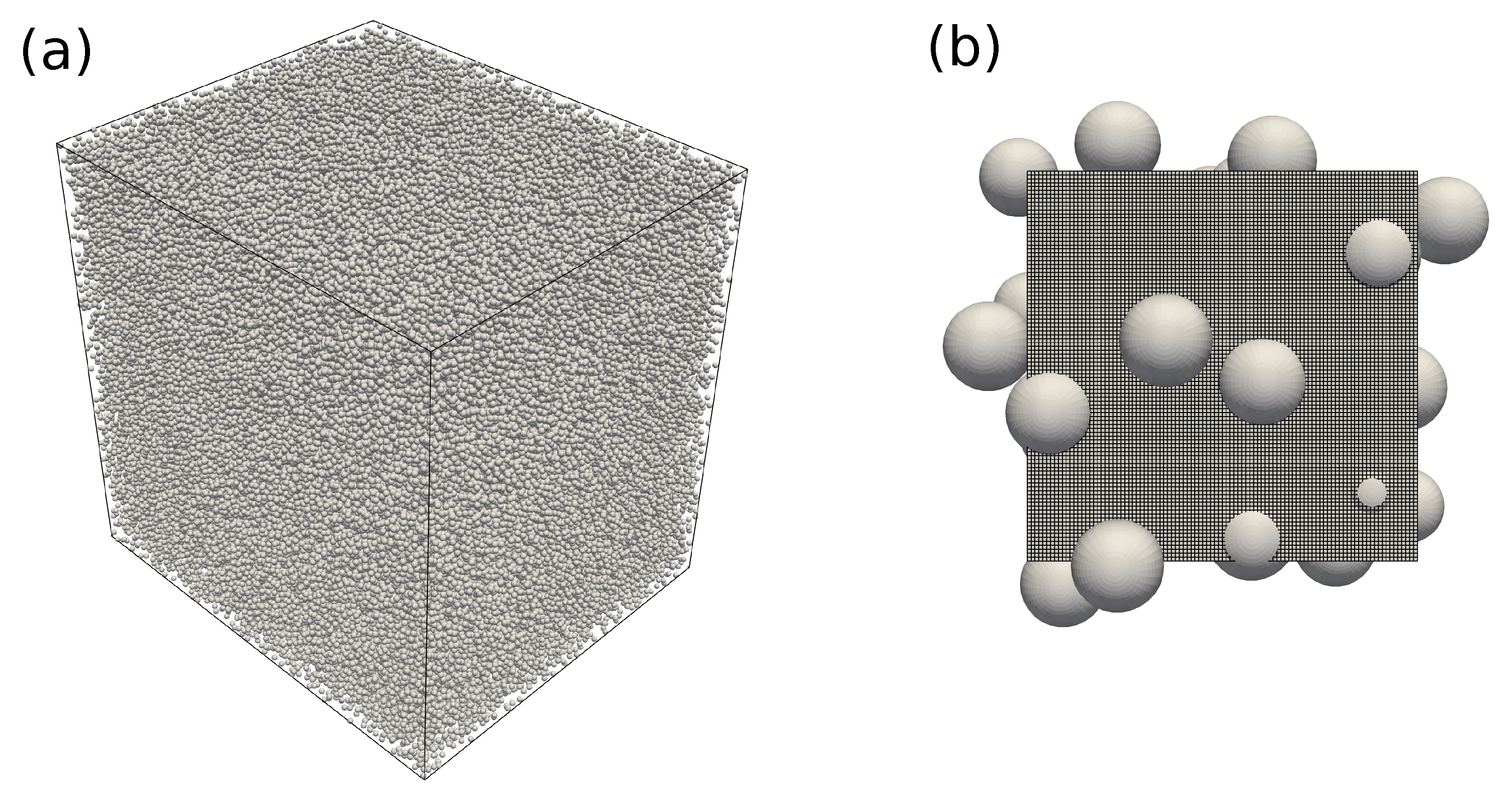
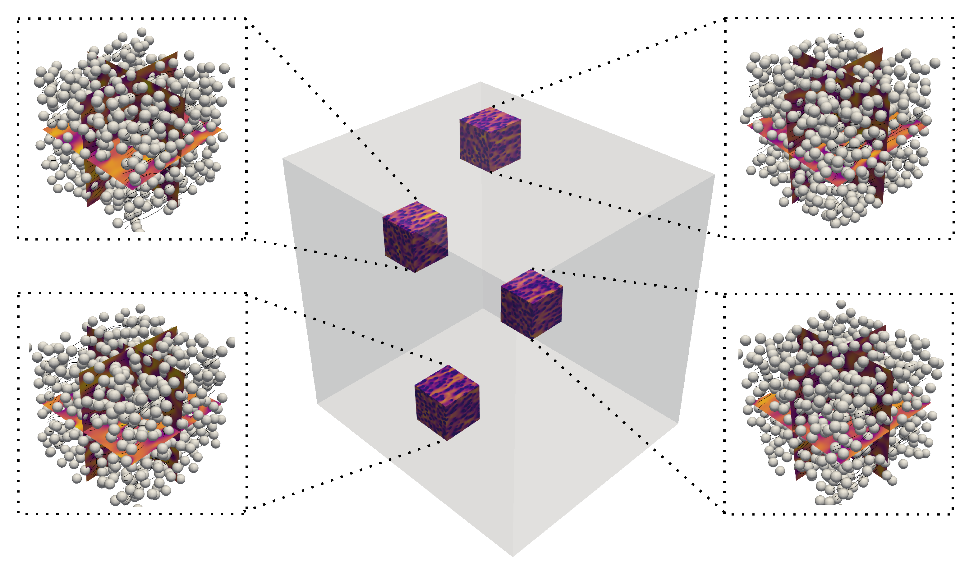
5. Massively Parallel Computing: Flow through a Random Array of Spheres

In this test case, we study the flow in a complex configuration of randomly generated spheres. Data of similar computations have been used recently for estimating and predicting force fluctuations using probability-driven point-particle model [39] and physics-inspired neural network [40,41]. The models are advanced in estimating the force fluctuations and providing an overall framework. Still, they need large datasets due to the curse of dimensionality and often risk over-prediction of the force coefficients. The particle-resolved direct numerical simulations of flow past a random array of spheres are computationally expensive using a solver based on a projection algorithm [19], which only generates O ( 1000 ) data points without losing the computational efficiency on many cores. Our Direction Splitting algorithm scales till ∼7000 cores contrary to the scaling (∼500 cores) of the projection algorithm, which motivates us to generate O(100,000) data points from only one simulation using our DS solver (equivalent to the data points of 100 simulations using a projection solver).
We randomly generate 144,327 spheres in a computational domain periodic in each x, y and z direction as illustrated in Figure 27a. The size of the computational domain is 71.4 d p × 84 d p × 84 d p where d p denotes the sphere diameter. The resulting solid void fraction is ϕ = 0.15 . We impose a constant pressure gradient in the x-direction to generate a steady flow at Reynolds number R e = 19.2 where R e is computed with d p and the average streamwise x velocity component. The rigid spheres are resolved on the computational grid with 24 grid points per sphere diameter. In a companion paper to appear soon, we have validated the DS solver for multiple flow configurations, including the flow past a random array of spheres, and a grid resolution of 20 to 40 points per diameter has proven to provide converged results for R e < 50 . Figure 27b shows a domain section with the computational grid and randomly generated spheres. The 24 grid points per sphere diameter spatial resolution results in a total number of grid cells of 1700 × 2000 × 2000 = 6.8 billion, corresponding to 6.8 billion and 20.4 billion degrees of freedom for pressure (p) and velocity ( u , v , w ), respectively. We use 6800 computing cores on the high-performance computing platform Sockeye available at the University of British Columbia and accordingly distribute 1 million grid cells in each sub-domain, i.e., on each core. A non-dimensional time-step of 10 3 is used for the time iterations, and a steady state is defined when the relative change of the L 2 norm of the flow field drops below 10 3 . The computation took less than two days to complete and such an extremely large data set is unprecedented in the literature as far as the authors of this paper know. To show that our solver indeed scales very well, we report in Table 2 weak scaling results. Each node on Sockeye comprises 40 cores and we compute two additional similar flow configurations (i.e., same R e = 19.2 and same ϕ = 0.15 ) but on a smaller domain where the load of 1 million grid cells per sub-domain is maintained. We report in the fifth column of Table 2 the average run time per time step for the three flow domains. On 170 nodes, our solver still performs very well and the scalability is 9.279 / 12.18 0.76 when compared to the computation on 1 node.
The large and rich data set we generate in the largest flow configuration with 144,327 spheres enables to plot very accurate probability density functions of force and torque distributions, and should be able to partly solve the problem of paucity of data when training advanced data-driven models of force and torque fluctuations.
Figure 28 shows the flow profile around the rigid spheres at a steady state. The complexity of the overall flow field is not evident due to the large-scale simulation. So multiple clipped sections, each accounting for 0.4 % of the computational domain, are shown in the sub-figures with the streamlines and flow profile on the orthogonal planes. The objective of this section is not to carry out a detailed analysis of this unique data set, which would go far beyond the scope of the present paper, but to illustrate the potential of our DS solver to perform computations on O ( 10 , 000 ) cores and O ( 10 10 ) grid cells. This opens up unprecedented opportunities to efficiently produce huge data sets of flows past random arrays of obstacles.

6. Conclusions and Perspectives

We implemented the Direction Splitting method of Keating and Minev in our platform PacIFiC to solve the incompressible Navier-Stokes equations in a flow domain with a complex geometry and created a workflow that enables us to import complex geometries via external STL files. We successfully validated the workflow on various test cases including a test case where we combine the consideration of fixed boundaries described by a STL file and a freely moving rigid body described by an analytical function. We also examine the large scale computing capabilities of the Direction Splitting method in a test case with complex boundaries that is multiple times larger than the largest single phase flow test case presented in [31].
Overall, our implementation of the Direction Splitting method that allows the description of complex geometries via STL files has been shown to be accurate, reliable and efficient. Such an implementation opens up unprecedented opportunities for large-scale computing in complex geometries. A companion paper to appear soon aims at providing more details and additional validation tests on our implementation of the Direction Splitting method. Future work in our group will target to use the Direction Splitting solver to produce data in various particle-laden flow configurations and analyse these data to infer new physical understanding, as well as coupling it to an Immersed Boundary Method and a solver for deformable biological capsules in order to compute the transport of red blood cells in complex network of capillaries [33].

Author Contributions

Conceptualization, A.W.; methodology, A.M. and A.G.; software, A.M., A.G. and A.W.; validation, A.M. and A.G.; investigation, A.M. and A.G.; resources, A.W.; writing—original draft preparation, A.M. and A.G.; writing—review and editing, A.W.; visualization, A.M. and A.G.; supervision, A.W.; project administration, A.W.; funding acquisition, A.W. All authors have read and agreed to the published version of the manuscript.

Funding

This research was funded by the Natural Sciences and Engineering Research Council of Canada (NSERC) via Anthony Wachs’ New Frontiers in Research Fund grant NFRFE-2018-01922.

Data Availability Statement

The data presented in this study are available on request from the corresponding author.

Acknowledgments

This research was enabled by support provided by Compute Canada through Anthony Wachs’s 2020 and 2021 Computing Resources for Research Groups allocation qpf-764-ac. This research was also supported through computational resources and services provided by Advanced Research Computing at the University of British Columbia.

Conflicts of Interest

The authors declare no conflict of interest. The funders had no role in the design of the study; in the collection, analyses, or interpretation of data; in the writing of the manuscript, or in the decision to publish the results.

References

  1. Glowinski, R.; Le Tallec, P. Augmented Lagrangian and Operator-Splitting Methods in Nonlinear Mechanics; Society for Industrial and Applied Mathematics: Philadelphia, PA, USA, 1989. [Google Scholar]
  2. Glowinski, R. Finite element methods for incompressible viscous flow. Handb. Numer. Anal. 2003, 9, 3–1176. [Google Scholar]
  3. Chorin, A.J. Numerical solution of the Navier-Stokes equations. Math. Comput. 1968, 22, 745–762. [Google Scholar] [CrossRef]
  4. Armfield, S.; Street, R. An analysis and comparison of the time accuracy of fractional-step methods for the Navier–Stokes equations on staggered grids. Int. J. Numer. Methods Fluids 2002, 38, 255–282. [Google Scholar] [CrossRef]
  5. Guermond, J.L.; Minev, P.; Shen, J. An overview of projection methods for incompressible flows. Computer Methods Appl. Mech. Eng. 2006, 195, 6011–6045. [Google Scholar] [CrossRef] [Green Version]
  6. Falgout, R.D.; Yang, U.M. HYPRE: A Library of High Performance Preconditioners. In Computational Science—ICCS 2002. Lecture Notes in Computer Science; Sloot, P.M.A., Hoekstra, A.G., Tan, C.J.K., Dongarra, J.J., Eds.; Springer: Berlin/Heidelberg, Germany, 2002; Volume 2331. [Google Scholar] [CrossRef] [Green Version]
  7. Ghia, U.; Ghia, K.N.; Shin, C. High-Re solutions for incompressible flow using the Navier-Stokes equations and a multigrid method. J. Comput. Phys. 1982, 48, 387–411. [Google Scholar] [CrossRef]
  8. Thompson, M.C.; Ferziger, J.H. An adaptive multigrid technique for the incompressible Navier-Stokes equations. J. Comput. Phys. 1989, 82, 94–121. [Google Scholar] [CrossRef]
  9. Popinet, S. A quadtree-adaptive multigrid solver for the Serre–Green–Naghdi equations. J. Comput. Phys. 2015, 302, 336–358. [Google Scholar] [CrossRef] [Green Version]
  10. Eymard, R.; Gallouët, T.; Herbin, R. Finite volume methods. Handb. Numer. Anal. 2000, 7, 713–1018. [Google Scholar]
  11. Wachs, A. Particle-scale computational approaches to model dry and saturated granular flows of non-Brownian, non-cohesive, and non-spherical rigid bodies. Acta Mech. 2019, 230, 1919–1980. [Google Scholar] [CrossRef]
  12. Peskin, C. The immersed boundary method. Acta Numer. 2002, 11, 479–517. [Google Scholar] [CrossRef] [Green Version]
  13. Mittal, R.; Iaccarino, G. Immersed boundary methods. Annu. Rev. Fluid Mech. 2005, 37, 239–261. [Google Scholar] [CrossRef] [Green Version]
  14. Mohd-Yusof, J. Combined Immersed Boundaries/B-Splines Methods for Simulations of Flows in Complex Geometries; Technical Report, CTR Annual Research Brief; Stanford University: Stanford, CA, USA, 1997. [Google Scholar]
  15. Roma, A.; Peskin, C.; Berger, M. An adaptive version of the immersed boundary method. J. Comput. Phys. 1999, 153, 509–534. [Google Scholar] [CrossRef] [Green Version]
  16. Uhlmann, M. An immersed boundary method with direct forcing for the simulation of particulate flows. J. Comput. Phys. 2005, 209, 448–476. [Google Scholar] [CrossRef] [Green Version]
  17. Glowinski, R.; Pan, T.; Hesla, T.; Joseph, D. A distributed Lagrange multiplier/fictitious domain method for particulate flows. Int. J. Multiph. Flow 1999, 25, 755–794. [Google Scholar] [CrossRef]
  18. Yu, Z.; Shao, X.; Wachs, A. A fictitious domain method for particulate flows with heat transfer. J. Comput. Phys. 2006, 217, 424–452. [Google Scholar] [CrossRef]
  19. Wachs, A.; Hammouti, A.; Vinay, G.; Rahmani, M. Accuracy of Finite Volume/Staggered Grid Distributed Lagrange Multiplier/Fictitious Domain simulations of particulate flows. Comput. Fluids 2015, 115, 154–172. [Google Scholar] [CrossRef]
  20. Selcuk, C.; Ghigo, A.R.; Popinet, S.; Wachs, A. A fictitious domain method with distributed Lagrange multipliers on adaptive quad/octrees for the direct numerical simulation of particle-laden flows. J. Comput. Phys. 2021, 430, 109954. [Google Scholar] [CrossRef]
  21. Ritz, J.; Caltagirone, J. A numerical continuous model for the hydrodynamics of fluid particle systems. Int. J. Numer. Methods Fluids 1999, 30, 1067–1090. [Google Scholar] [CrossRef]
  22. Vincent, S.; Brändle de Motta, J.; Sarthou, A.; Estivalezes, J.L.; Simonin, O.; Climent, E. A Lagrangian VOF tensorial penalty method for the DNS of resolved particle-laden flows. J. Comput. Phys. 2014, 256, 582–614. [Google Scholar] [CrossRef] [Green Version]
  23. Chung, M.H. Cartesian cut cell approach for simulating incompressible flows with rigid bodies of arbitrary shape. Comput. Fluids 2006, 35, 607–623. [Google Scholar] [CrossRef]
  24. Hartmann, D.; Meinke, M.; Schröder, W. A strictly conservative Cartesian cut-cell method for compressible viscous flows on adaptive grids. Comput. Methods Appl. Mech. Eng. 2011, 200, 1038–1052. [Google Scholar] [CrossRef]
  25. Meinke, M.; Schneiders, L.; Günther, C.; Schröder, W. A cut-cell method for sharp moving boundaries in Cartesian grids. Comput. Fluids 2013, 85, 135–142. [Google Scholar] [CrossRef]
  26. Keating, J.; Minev, P. A fast algorithm for direct simulation of particulate flows using conforming grids. J. Comput. Phys. 2013, 255, 486–501. [Google Scholar] [CrossRef]
  27. Peaceman, D.W.; Rachford Jr., H.H. The numerical solution of parabolic and elliptic differential equations. J. Soc. Ind. Appl. Math. 1955, 3, 28–41. [Google Scholar] [CrossRef]
  28. Douglas, J. Alternating direction methods for three space variables. Numer. Math. 1962, 4, 41–63. [Google Scholar] [CrossRef]
  29. Yu, Z.; Phan-Thien, N.; Tanner, R. Dynamic simulation of sphere motion in a vertical tube. J. Fluid Mech. 2004, 518, 61–93. [Google Scholar] [CrossRef]
  30. Guermond, J.; Minev, P. A new class of massively parallel direction splitting for the incompressible Navier–Stokes equations. Comput. Methods Appl. Mech. Eng. 2011, 200, 2083–2093. [Google Scholar] [CrossRef]
  31. Guermond, J.; Minev, P. Start-up flow in a three-dimensional lid-driven cavity by means of a massively parallel direction splitting algorithm. Int. J. Numer. Methods Fluids 2012, 68, 856–871. [Google Scholar] [CrossRef]
  32. Guermond, J.L.; Shen, J. Velocity-Correction Projection Methods for Incompressible Flows. SIAM J. Numer. Anal. 2003, 41, 112–134. [Google Scholar] [CrossRef]
  33. Balogh, P.; Bagchi, P. A computational approach to modeling cellular-scale blood flow in complex geometry. J. Comput. Phys. 2017, 334, 280–307. [Google Scholar] [CrossRef] [Green Version]
  34. Mehmani, Y.; Tchelepi, H.A. Minimum requirements for predictive pore-network modeling of solute transport in micromodels. Adv. Water Resour. 2017, 108, 83–98. [Google Scholar] [CrossRef]
  35. Geuzaine, C.; Remacle, J.F. Gmsh: A 3-D finite element mesh generator with built-in pre-and post-processing facilities. Int. J. Numer. Methods Eng. 2009, 79, 1309–1331. [Google Scholar] [CrossRef]
  36. Paul, F.; Fischer, J.W.L.; Kerkemeier, S.G. nek5000 Web Page. 2008. Available online: http://nek5000.mcs.anl.gov (accessed on 1 June 2022).
  37. Patera, A.T. A spectral element method for fluid dynamics: Laminar flow in a channel expansion. J. Comput. Phys. 1984, 54, 468–488. [Google Scholar] [CrossRef]
  38. Segre, G.; Silberberg, A. Behaviour of macroscopic rigid spheres in Poiseuille flow Part 2. Experimental results and interpretation. J. Fluid Mech. 1962, 14, 136–157. [Google Scholar] [CrossRef]
  39. Seyed-Ahmadi, A.; Wachs, A. Microstructure-informed probability-driven point-particle model for hydrodynamic forces and torques in particle-laden flows. J. Fluid Mech. 2020, 900, A21. [Google Scholar] [CrossRef]
  40. Seyed-Ahmadi, A.; Wachs, A. Physics-inspired architecture for neural network modeling of forces and torques in particle-laden flows. Comput. Fluids 2022, 238, 105379. [Google Scholar] [CrossRef]
  41. Siddani, B.; Balachandar, S. Point-particle drag, lift, and torque closure models using machine learning: Hierarchical approach and interpretability. Phys. Rev. Fluids 2022, 8, 014303. [Google Scholar] [CrossRef]
Figure 1. Definition of the current framework. The fluid domain and the solid domain are defined by Ω f and Ω s , respectively. d Ω denotes the fluid-solid interface.
Fluids 08 00086 g001
Figure 2. STL file of a blood vessel positioned in a cuboid computational domain. The blue dots correspond to the field (i.e., u x , u y , u z , p ) nodes.
Fluids 08 00086 g002
Figure 3. Ray-tracing approach employed for two nodes located at ( x 1 , y 1 , z 1 ) and ( x 2 , y 2 , z 2 ) : (a) front and (b) top-left views of the blood vessel.
Fluids 08 00086 g003
Figure 4. Computation of the distances between the grid node and the intersecting triangles in both x and y directions denoted respectively d x and d y .
Fluids 08 00086 g004
Figure 5. (a) Subdivision of the computational domain along y into 5 subdivisions: H x 1 , , H x 5 . If a node belongs to H x 3 , the loop over the set of triangles is reduced to the triangles belonging to H x 3 . (b) Subdivision of the computational domain along x into 3 subdivisions: H y 1 , , H y 2 . If a node belongs to H y 2 , the loop over the set of triangles is reduced to the triangles belonging to H y 2 .
Fluids 08 00086 g005
Figure 6. STL triangulations of the pipe wall, left to right: D c / Δ c t = 6 , 24 and 96.
Fluids 08 00086 g006
Figure 7. Influence of the grid refinement D c / Δ x = 6 , 12 , 24 , 48 and 96 on the convergence of the velocity profiles: (a) D c / Δ c t = 6 , (b) D c / Δ c t = 24 , (c) D c / Δ c t = 96 .
Fluids 08 00086 g007
Figure 8. Influence of the triangle characteristic size Δ c t on the convergence of the velocity profiles: (a) D c / Δ x = 6 , (b) D c / Δ x = 24 , (c) D c / Δ x = 48 .
Fluids 08 00086 g008
Figure 9. Combined influence of the ratios D c / Δ c t and D c / Δ x on the convergence of the method.
Fluids 08 00086 g009
Figure 10. (a) STL triangulation corresponding to the semi-wavy configuration in x and y directions considered for the simulations, (b) computational domain used in Nek5000.
Fluids 08 00086 g010
Figure 11. Contours of u x / | | u x N e k | | at the steady state on a plane located at z = 1.19 orthogonal to the z axis. Left: Nek5000, right: Direction Splitting, h s / Δ x = 96 .
Fluids 08 00086 g011
Figure 12. Contours of u y / | | u y N e k | | at the steady state on a plane located at y = 0.19 orthogonal to the z axis. Left: Nek5000, right: Direction Splitting, h s / Δ x = 96 .
Fluids 08 00086 g012
Figure 13. Contours of u x / | | u x N e k | | at the steady state on a plane located at y = 0.15 orthogonal to the y axis. Left: Nek5000, right: Direction Splitting, h s / Δ x = 96 .
Fluids 08 00086 g013
Figure 14. Contours of u z / | | u z N e k | | at the steady state on a plane located at y = 0.15 orthogonal to the y axis. Left: Nek5000, right: Direction Splitting, h s / Δ x = 96 .
Fluids 08 00086 g014
Figure 15. Definition of the 1D profiles used for the comparison with Nek5000.
Fluids 08 00086 g015
Figure 16. Profiles of u x , u y and u z for h / Δ x = 24 , 48 , 96 along the wall-normal direction, profile set at ( x 1 , z 1 ) .
Fluids 08 00086 g016
Figure 17. Profiles of u x , u y and u z for h / Δ x = 24 , 48 , 96 along the wall-normal direction, profile set at ( x 2 , z 2 ) .
Fluids 08 00086 g017
Figure 19. STL triangulation of the sandstone rock used in the simulations: (a) x y view and (b) y z view showing a single triangle in the z direction.
Fluids 08 00086 g019
Figure 20. Sketch of the flow configuration: (a) upstream part of the domain without any buffer region and (b) full domain with inlet and outlet buffer regions and a thin layer removed in the y direction.
Fluids 08 00086 g020
Figure 21. Contours of | | u | | 2 (in m/s) at the steady state. The STL triangulation is also shown here in light gray. (a) Whole computational domain, (b) zoomed view of the purple square as shown in (a).
Fluids 08 00086 g021
Figure 22. Influence of the grid refinement on the permeability coefficient k.
Fluids 08 00086 g022
Figure 23. STL triangulation of the pipe wall used in the simulations.
Fluids 08 00086 g023
Figure 24. Snapshot of | | u | | 2 / | | u | | for R e = 115 and ( x p / R c , y p / R c , z p / R c ) = ( 1 , 0.5 , 0 ) as the initial position of the particle in the pipe.
Fluids 08 00086 g024
Figure 25. Trajectory of the particle in the x y plane, sequenced as periods (colored lines). (a) R e = 12 , (b) R e = 115 . The red cross indicates the initial particle position, the bold black lines correspond to the pipe interface, and the dashed black line correspond to the centerline of the pipe.
Fluids 08 00086 g025
Figure 26. Trajectory of the particle in the x y plane, sequenced as periods (colored lines), case R e = 113 . The red cross indicates the initial particle position, the bold black lines correspond to the pipe interface, and the dashed black line correspond to the centerline of the pipe.
Fluids 08 00086 g026
Figure 27. (a) Computational domain showing all rigid spheres. (b) Sub-domain on a single computing core showing well-resolved spheres with a grid resolution of 24 grid points per diameter.
Fluids 08 00086 g027
Figure 28. Flow visualization in multiple sub-domains at the steady state. The streamlines and rigid spheres for each sub-domain are shown in the sub-images.
Fluids 08 00086 g028
Table 1. Wall-time ( s e c ) of the pre-step for small, medium and large triangulations, and an increasing number of subdivisions, ranging from N s = 1 to N s = 20 .
Number of Triangles N s = 1 N s = 5 N s = 10 N s = 20
20 × 10 3 300.2185.22.2
100 × 10 3 550.745.135.215.2
200 × 10 3 920.910878.455.2
Table 2. Weak scaling results in the flow through a random array of spheres at R e = 19.2 and ϕ = 0.15 .
Number of NodesNumber of CoresNumber of CellsNumber of SpheresRun Time per Time Step (s)
14040,000,0008499.279
8320320,000,00067929.924
17068006,800,000,000144,32712.18
Disclaimer/Publisher’s Note: The statements, opinions and data contained in all publications are solely those of the individual author(s) and contributor(s) and not of MDPI and/or the editor(s). MDPI and/or the editor(s) disclaim responsibility for any injury to people or property resulting from any ideas, methods, instructions or products referred to in the content.

