Modal Representation of Inertial Effects in Fluid–Particle Interactions and the Regularity of the Memory Kernels

Abstract

This article develops a modal expansion (in terms of functions exponentially decaying with time) of the force acting on a micrometric particle and stemming from fluid inertial effects (usually referred to as the Basset force) deriving from the application of the time-dependent Stokes equation to model fluid–particle interactions. One of the main results is that viscoelastic effects induce the regularization of the inertial memory kernels at $t=0$, eliminating the $1/\sqrt{t}$-singularity characterizing Newtonian fluids. The physical origin of this regularization stems from the finite propagation velocity of the internal shear stresses characterizing viscoelastic constitutive equations. The analytical expression for the fluid inertial kernel is derived for a Maxwell fluid, and a general method is proposed to obtain accurate approximations of it for generic complex viscoelastic fluids, characterized by a spectrum of relaxation times.

1. Introduction

Microfluidics and the study of fluid–particle interactions at a microscale represent not only a vast area of practical engineering applications [1,2] as they provide the opportunity of addressing fundamental physical questions in fluid dynamics [3,4,5], such as the relevance of acoustic propagation in liquid hydrodynamics [6,7,8], the nature of the boundary conditions and the occurrence of slip effects [9,10,11], as well as the role of the finite propagation velocity in the evolution of internal stresses [8,12].

A significant role in this research is played by the study, both theoretical and experimental, of Brownian motion, i.e., of the motion of micrometric particles in a quiescent fluid. This is due to the fact that Brownian motion is a central problem in statistical physics, from the early age of Einstein, Langevin, Smoluchowski, Perrin, [13,14,15,16] up to now [17,18], providing a direct way of quantifying the influence of thermal fluctuations and of studying the interactions between a fluid and a particle, thus permitting the investigation of the role and the relative relevance of different hydrodynamic effects. In this sense, Brownian motion represents an invaluable probe to verify experimentally fundamental fluid dynamic properties at short time and length scales [11,19].

The last two decades have seen an increasing attention on the experimental analysis of Brownian motion at short time scales in different fluids (gases and liquids) [20,21,22,23,24], with different rheological properties (Newtonian, viscoelastic) [25]. The experimental results have confirmed many predictions of the hydrodynamic theory of Brownian motion [26,27,28], and in some cases have raised fundamental questions involving basic principles of statistical mechanics [29].

The analysis of the velocity autocorrelation function of a micrometric particle in a liquid phase has shown the importance of fluid inertial contributions, expressed by the occurrence of the Basset force and of the added-mass term [30] in the expression of the force exerted by a fluid on a rigid object [22,23]. These terms arise in the low-Reynolds number hydrodynamics, using the time-dependent Stokes equations, and provide a power-law decay of the particle velocity autocorrelation function [25], to be compared with the exponential decay occurring if solely the Stokesian drag is considered [31,32]. Indeed, the use of the time-dependent Stokes equation, instead of the instantaneous Stokes formulation, is well justified and appropriate when addressing micrometric particle motion in liquids at short time scale, due to the high frequencies characterizing thermal fluctuations. Consequently, while the Reynolds number is extremely small in these systems, the product of the Reynolds number times the Strouhal numbers is order of unity, justifying the inclusion of the inertial contribution expressed as the time derivative of the velocity in the hydrodynamic equations. In the case of viscoelastic fluids, characterized by time-dependent constitutive equations, this statement is a fortiori valid.

The rheological modeling of complex viscoelastic fluids is well consolidated as regards the quantitative description of viscoelastic properties [33]. As regards the dynamics of a microparticle, this corresponds to the formulation of a generalized Langevin equation with a dissipative memory kernel [34,35,36]. This class of equations has been introduced by Zwanzig in connection with the interaction of a physical system with a heat bath, and the fluctuation–dissipation theorem for this class of systems has been obtained by Kubo [37]. On the other hand, the hydrodynamic analysis of Brownian motion and the numerical simulation experiments by Alder and Wainwright [38] have clearly indicated that fluid inertial contributions are of paramount importance in order to correctly predict particle dynamics.

The current approach to particle motion in complex fluids is essentially based on the direct hydrodynamic simulation of particle motion [39,40]. What is missing is a physically consistent and computationally tractable formulation of particle dynamics in viscoelastic fluids, analogous to the corresponding equation of motion (which includes Stokes friction, the Basset force and the added mass effect) that apply for Newtonian ones. These equations can be derived into two steps: (i) via the detailed characterization of the fluid inertial contribution to particle motion in a complex fluid, expressing it in a computationally effective representation, and (ii) by generalizing the Kubo fluctuation–dissipation theory in order to include fluid-inertial contributions. In this article, we focus essentially on the first issue, leaving the second one to a forthcoming work.

Albeit the present analysis is focused on the hydrodynamic theory of particle motion, its application to microfluidic engineering for particle separation and nanoparticle production and optimization is significant. Indeed, the obtained result could be directly applied to the design of microfluidic systems enforcing the rheological properties of complex fluids in the limit of Stokesian hydrodynamics. In point of fact, the importance of inertial effects and rheological properties in separation devices is well known, e.g., in connection with the Segré-Silberberg effect [40,41], although this effect involves flows at non-vanishing Reynolds numbers [4,42].

The aim of this article is two-fold. A first goal involves the development of the modal representation of the fluid inertial contributions in the expression of the particle equation of motion in a fluid phase. This naturally leads to a simple field-theoretical representation of these effects. The second goal involves the mathematical structure of the inertial memory kernels entering the convolutional representation of the Basset forces, and their basic qualitative properties derived from fundamental physical principles. Specifically, it is shown that for any viscoelastic fluid (and all the liquids fall in this category, even if their characteristic relaxation times could be extremely small), the inertial memory kernel accounting for the generalized Basset contribution is bounded and non-singular near time $t=0$.

The article is organized as follows. Section 2 introduces the hydrodynamic problem, the representation of fluid inertial effects and their implications in microparticle dynamics. Section 3 analyzes the modal representation of the Basset force, and its compact description in terms of a simple field equation. Moreover, it is shown in Section 3.2 that the modal representation also provides an efficient computational tool to study inertial particle motion. This is an important topic that recently emerged in the fluid-dynamic literature [43,44,45] in connection with the numerical solution of the Maxey–Riley equation [46] (see also [47] and references therein). Specifically, the modal expansion transforms the integro-differential equations of motion into a system of ordinary differential equations. Section 4 addresses the boundedness of the resulting memory kernels in the presence of viscoelastic constitutive equations, outlining the physical and computational relevance of this result. For a simple Maxwell fluid, the expression of this kernel is obtained in closed form, and a general method for approximating it for generic complex viscoelastic fluids is proposed. Finally, Section 4.3 describes the connection between the present theory and the generalization of the Kubo fluctuation–dissipation theory to include fluid inertial effects in the stochastic equations of motion for a microparticle in a heat bath at constant temperature.

2. Fluid–Particle Interactions and Inertial Effects

Consider the motion of a micrometric rigid spherical particle of radius R in a unbounded incompressible fluid. Assume that the fluid is Newtonian, and $\rho$ and $\mu$ represent its density and viscosity, respectively. Without loss of generality, assume neutrally buoyant particles (i.e., possessing the same density as the liquid), as the inclusion of Archimedean forces is immaterial in the present analysis. Let $B_R$ be the domain representing the space occupied by the particle, $\partial B_R$ its boundary and ${\mathbf{V}}_p\left(t\right)$ its translational velocity. Since we are considering the motion of a Brownian particle in a still liquid (the liquid is referred to be still if its velocity field originates exclusively from thermal motion of the immersed Brownian particle), the momentum balance equation for the particle reads

$$m\frac{d{\mathbf{V}}_p\left(t\right)}{dt}={\mathbf{F}}_{f\to p}\left[{\mathbf{V}}_p\left(t\right)\right]+\mathbf{S}\left(t\right)$$

(1)

where ${\mathbf{F}}_{f\to p}\left[{\mathbf{V}}_p\left(t\right)\right]$ represents the force exerted by the fluid on the particle, and is a functional of the particle velocity, expressed by the surface integral over $\partial B_R$,

$${\mathbf{F}}_{f\to p}\left[{\mathbf{V}}_p\left(t\right)\right]=-{\int }_{\partial B_R}\left(\mathbf{\tau }+p\mathbf{I}\right)·{\mathbf{e}}_{r}dS$$

(2)

where $\tau$ is the shear stress tensor, p the pressure, $\mathbf{I}$ the identity matrix and ${\mathbf{e}}_r$ is the unit radial vector (we consider a reference system with the origin at the center of the spherical particle) and $\mathbf{S}\left(t\right)$ is a stochastic contribution describing the thermal force fluctuation.

Indicating with $\mathbf{v}(\mathbf{x},t)$ the fluid velocity field, in the low-Reynolds number regime it is the solution of the time-dependent Stokes equations

$$\rho \frac{\partial \mathbf{v}}{\partial t}=-\nabla ·\mathbf{\tau }-\nabla p,\nabla ·\mathbf{v}=0,\mathbf{x}\in {\mathbb{R}}^3/B_R$$

(3)

equipped with the boundary and initial conditions,

$${\mathbf{v}(\mathbf{x},t)|}_{\mathbf{x}\in \partial B_R}={\mathbf{V}}_p{\left(t\right),\mathbf{v}(\mathbf{x},t)|}_{t=0}=0$$

(4)

Equation (4) corresponds to the no-slip assumption. For an incompressible Newtonian fluid,

$$\mathbf{\tau }=-\mu \left(\nabla \mathbf{v}+\nabla {\mathbf{v}}^T\right)$$

(5)

where the superscript “T” indicates transpose, so that Equation (3) is a linear partial differential equation for $\mathbf{v}(\mathbf{x},t)$ (the time-dependent Stokes equation)

$$\rho \frac{\partial \mathbf{v}}{\partial t}=\mu {\nabla }^2\mathbf{v}-\nabla p$$

(6)

where, from Equation (3), the velocity field $\mathbf{v}(\mathbf{x},t)$ is incompressible. Owing to the linearity of Equations (5) and (6), the functional ${\mathbf{F}}_{f\to p}\left[{\mathbf{V}}_p\right]$ is a linear and causal functional of the particle velocity ${\mathbf{V}}_p\left(t\right)$. Causality means that ${\mathbf{F}}_{f\to p}\left[{\mathbf{V}}_p\left(t\right)\right]$ depends solely on the velocity history in the interval $[0,t)$.

Under these conditions, the force exerted by the fluid onto the rigid spherical particle can be expressed analytically. Let us indicate with ${\widehat{\mathbf{F}}}_{f\to p}\left(s\right)$ the Laplace transform of ${\mathbf{F}}_{f\to p}\left[{\mathbf{V}}_p\right]$ (henceforth, we will indicate with $\widehat{f}\left(s\right)={\int }_0^{\infty }{e}^{-st}f\left(t\right)dt$ the Laplace transform of any function $f\left(t\right)$ of time t, and with s the complex-valued Laplace variable), ${\widehat{\mathbf{F}}}_{f\to p}\left(s\right)$ attains the expression [48,49]

$$-{\widehat{\mathbf{F}}}_{f\to p}\left(s\right)=6\pi \mu R{\widehat{\mathbf{V}}}_p\left(s\right)+6\pi \sqrt{\frac{\rho \mu }{s}}{R}^2\left(s{\widehat{\mathbf{V}}}_p\left(s\right)\right)+\frac{2}{3}\rho \pi R^3\left(s{\widehat{\mathbf{V}}}_p\left(s\right)\right)$$

(7)

Transforming Equation (7) back into the time domain, one obtains

$$\begin{array}{ccc}\hfill & & {\mathbf{F}}_{f\to p}\left[{\mathbf{V}}_p\left(t\right)\right]=-6\pi \mu R{\mathbf{V}}_p\left(t\right)\hfill \\ & & -6\sqrt{\pi \rho \mu }{R}_p^2{\int }_0^t\frac{1}{\sqrt{t-\tau }}\left(\frac{d{\mathbf{V}}_p\left(\tau \right)}{d\tau }+{\mathbf{V}}_p\left(0\right)\delta \left(\tau \right)\right)d\tau -\frac{2}{3}\rho \pi R^3\frac{d{\mathbf{V}}_p\left(t\right)}{dt}\hfill \end{array}$$

(8)

where ${\mathbf{V}}_p\left(0\right)$ is the initial condition for the particle velocity at $t=0$. The first term at the r.h.s. of Equation (8) is the Stokesian friction, with the factor $\eta =6\pi \mu R$, corresponding to the only dissipative term occurring also in the case of the instantaneous Stokes regime. The two other contributions at the r.h.s. stem from fluid inertial effects, and depend on the history of particle acceleration up to time t. The first of these terms is the convolutional integral of $d{\mathbf{V}}_p\left(t\right)/dt$ with the kernel $k\left(t\right)$ given by

$$k\left(t\right)=\frac{6\sqrt{\pi \rho \mu }{R}^2}{\sqrt{t}}$$

(9)

and it is usually referred to as the Basset force. Let us observe that kernel $k\left(t\right)$ is singular at $t=0$. This property will be thoroughly analyzed in Section 4. The last term at the r.h.s. of Equation (8) is an instantaneous inertial contribution proportional to the actual value (i.e., at time t) of the acceleration $d{\mathbf{V}}_p\left(t\right)/dt$ of the particle, and it defines the hydrodynamic added mass $m_a=2\rho \pi R^3/3$, equal to half of the mass of the fluid displaced by the particle [31]. Let us observe within the Basset term the occurrence of a contribution proportional to ${\mathbf{V}}_p\left(0\right)\delta \left(\tau \right)$, in the case ${\mathbf{V}}_p\left(0\right)\ne 0$. Equation (8) can be compactly written as

$$m_e\frac{d{\mathbf{V}}_p\left(t\right)}{dt}=-\eta {\mathbf{V}}_p\left(t\right)-k\left(t\right)\ast \left(\frac{d{V}_p\left(t\right)}{dt}+V_p\left(0\right)\delta \left(t\right)\right)+\mathbf{S}\left(t\right)$$

(10)

where $m_e=m+m_a$ is the extended mass and “∗” indicates convolution. The physical importance of the Basset contribution can be appreciated by considering the velocity autocorrelation tensor of a Brownian particle, ${\mathbf{C}}_v\left(t\right)=\langle {\mathbf{V}}_p\left(t\right)\otimes {\mathbf{V}}_p\left(0\right)\rangle$, where “⊗” indicates the dyadic tensor product and “$\langle ·\rangle$” the ensemble average over the probability measure of the thermal fluctuations. Since $\langle \mathbf{S}\left(t\right)\otimes {\mathbf{V}}_p\left(0\right)\rangle =0$, as it is physically reasonable to assume that the thermal fluctuations $\mathbf{S}\left(t\right)$ at time $t\ge 0$, are independent of (uncorrelated to) the velocity fluctuations at any previous time instant $t=0$ [32,37] (this principle is by some authors referred to as the principle of causality [50], and it essentially states the non-anticipativity of the action of thermal fluctuations as regards its effects on the particle velocity), by taking the tensorial product of both members of Equation (10) and averaging over the statistics of thermal fluctuations (the operations of time derivative and convolution commute with $\langle ·\rangle$), we obtain the evolution equation for ${\mathbf{C}}_v\left(t\right)$,

$$m^{*}\frac{d{\mathbf{C}}_v\left(t\right)}{dt}=-\eta {\mathbf{C}}_v\left(t\right)-k\left(t\right)\ast \left(\frac{d{\mathbf{C}}_v\left(t\right)}{dt}+{\mathbf{C}}_v\left(0\right)\right)$$

(11)

equipped with the isotropic initial condition

$${\mathbf{C}}_v\left(0\right)=\langle V^2\rangle \mathbf{I}$$

(12)

where $\langle V^2\rangle$ is the squared variance of any entry $V_{p,h}\left(t\right)$, $h=1,2,3$ of the particle velocity vector (proportional at thermal equilibrium to the temperature of the fluid). Therefore, due to this symmetry, the velocity autocorrelation function can be expressed as ${\mathbf{C}}_v\left(t\right)=\langle V^2\rangle c_v\left(t\right)\mathbf{I}$, where the scalar function $c_v\left(t\right)$ satisfies Equation (11) with $c_v\left(0\right)=1$. The occurrence of the Basset contribution determines a qualitative change in the long-term scaling of $c_v\left(t\right)$ with respect to the purely dissipative case (corresponding to considering the fluid motion in an instantaneous Stokes flow). In the latter case, the long-term decay is exponential, i.e., $c_v\left(t\right)=e^{-\eta t/m}$ while inertial effects induce an asymptotic power-law scaling $c_v\left(t\right)\sim t^{-\gamma }$, with $\gamma =3/2$ in the free space [25,37].

The application of Equation (10) in the Lagrangian analysis of particle motion, in the case the kernel $k\left(t\right)$ attains the Basset form expressed by Equation (9), raises three main issues:

• A computational issue, as the presence of a convolution in the equations of motion implies that the entire history of ${\mathbf{V}}_p\left(t\right)$ over the time interval $[0,t)$ should be stored in order to evaluate it;
• An analytical issue, associated with the singularity of the Basset kernel $k\left(t\right)$ at $t=0$;
• A physical issue, related to the determination of the stochastic force $\mathbf{S}\left(t\right)$, in the case that inertial effects are accounted for.

The first problem is analyzed in the next section, in terms of modal representations. The second one is treated on physical grounds in Section 4. The last point, related to the determination of $\mathbf{S}\left(t\right)$, is one of the main issues of fluctuation–dissipation theories [32,37]. To the best of our knowledge, a computationally valid approach to the determination of $\mathbf{S}\left(t\right)$ in the presence of the Basset term is lacking, although formal results have been proposed [51]. This point will be addressed in forthcoming works, as it pertains mostly to statistical physics than to strict hydrodynamic theory.

3. Modal Representation

The idea behind modal representations lies in the expression of the fluid inertial memory term entering the particle equation of motion as a linear superposition of elementary stochastic modes, susceptible of a simple evolution. We use the diction “stochastic” in this context, to pinpoint the fact that since $\mathbf{S}\left(t\right)\ne 0$, the velocity ${\mathbf{V}}_p\left(t\right)$ is itself a stochastic process, as well as any other process functionally dependent on ${\mathbf{V}}_p\left(t\right)$.

Let us consider Equation (10), and without loss of generality let us set ${\mathbf{V}}_p\left(0\right)=0$. Since the problem of Brownian motion in the free space is isotropic, we can exclusively consider a scalar formulation of it, setting $V_p\left(t\right)$ instead of ${\mathbf{V}}_p\left(t\right)$. Let us assume in the remainder that the stochastic representation of $S\left(t\right)$ (replacing $\mathbf{S}\left(t\right)$ as a scalar formulation is considered) is known.

Consider a family of stochastic processes $y(t;\lambda )$ parameterized with respect to $\lambda \in [0,\infty )$ and fulfilling the equations

$$\frac{dy(t;\lambda )}{dt}=-\lambda y(t,\lambda )+q\frac{d{V}_p\left(t\right)}{dt}$$

(13)

where q is a constant to be determined. Let us suppose $y(t=0;\lambda )=0$ so that

$$y(t;\lambda )=q{\int }_0^t{e}^{-\lambda (t-\tau )}\frac{d{V}_p\left(\tau \right)}{d\tau }d\tau$$

(14)

The inertial memory kernel can be expressed as a linear superposition of these processes. To this end, let $p\left(\lambda \right)$ the probability density of occurrence of $y(t;\lambda )$, so that $p\left(\lambda \right)d\lambda$ represents the infinitesimal weight factor in the representation of the memory inertial contribution. Thus, the particle equation of motion can be expressed as

$$m^{*}\frac{d{V}_p\left(t\right)}{dt}=-\eta V_p\left(t\right)-\underset{I}{\underbrace{q{\int }_0^{\infty }p\left(\lambda \right)y(t;\lambda )d\lambda }}+S\left(t\right)$$

(15)

The integral I entering Equation (15) can be rewritten in convolutional form as

$$I={\int }_0^t\left[q{\int }_0^{\infty }p\left(\lambda \right)e^{-\lambda (t-\tau )}d\lambda \right]\frac{d{V}_p\left(\tau \right)}{d\tau }d\tau =k_p\left(t\right)\ast \frac{d{V}_p\left(t\right)}{dt}$$

(16)

thus defining the kernel $k_p\left(t\right)$.

Let us assume for $p\left(\lambda \right)$ the following expression

$$p\left(\lambda \right)=\left\{\begin{array}{ccc}A{\lambda }^{-1/2}& & \lambda <{\lambda }_c\hfill \\ 0& & \mathrm{otherwise}\hfill \end{array}\right.$$

(17)

where ${\lambda }_c>0$, and A is the normalization constant such that ${\int }_0^{\infty }p\left(\lambda \right)d\lambda =1$. In this case, setting $z={\lambda }_{c}t$,

$$k_p\left(t\right)=\frac{qA}{\sqrt{t}}{\int }_0^{{\lambda }_{c}t}\frac{e^{-z}}{\sqrt{z}}dz$$

(18)

Let us observe that $k_p\left(0\right)=q$, while for $t>0$, and for large ${\lambda }_c$, ${\lambda }_{c}t$ can be approximated by an infinite value, and thus

$$k_p\left(t\right)=\frac{qA}{\sqrt{t}}{\int }_0^{\infty }\frac{e^{-z}}{\sqrt{z}}dz=\frac{qA\pi }{\sqrt{t}}$$

(19)

The constant q can be always defined in order to match the asymptotics of the Basset kernel Equation (9). Therefore, the modal expansion Equation (15) provides an inertial kernel that does not match the singular behavior of the Basset kernel near $t=0$, but still represents an excellent approximation of it for t large enough. The regularity of the inertial kernel will be questioned in the next section starting from physical arguments.

If one is interested in obtaining exactly the modal expansion for the Basset kernel, a slightly different parameterization can be chosen by considering the modes $y(t;k)$, $k\in [0,\infty )$, still satisfying the linear relaxation dynamics Equation (13), with the relaxation rates $\lambda =\lambda \left(k\right)$ depending quadratically on the parameter k, i.e.,

$$\lambda \left(k\right)={\lambda }_0{k}^2$$

(20)

with ${\lambda }_0>0$, consequently,

$$y(t;k)=q{\int }_0^t{e}^{-k^2(t-\tau )}\frac{d{V}_p\left(\tau \right)}{d\tau }d\tau$$

(21)

Assuming that all the modes at different ks concur uniformly in the expansion of the inertial force, i.e., that the weight function does not have a probabilistic meaning, the integral I in the k-representation becomes

$$I={\int }_0^{\infty }y(t;k)dk=k_k\left(t\right)\ast \frac{d{V}_p\left(t\right)}{dt},k_k\left(t\right)=q{\int }_0^{\infty }{e}^{-{\lambda }_0{k}^{2}t}dk$$

(22)

providing

$$k_k\left(t\right)=\frac{q}{2}\sqrt{\frac{\pi }{{\lambda }_{0}t}}$$

(23)

and thus the parameters q and ${\lambda }_0$ can be always determined in order to exactly match the Basset kernel Equation (9).

3.1. Diffusional Field Representation

The quadratic spectral representation based on the dispersion relation Equation (20) suggests the Basset inertial term could be viewed as the consequence of the interaction of diffusional models associated with a scalar field with the particle. It is therefore interesting to further develop this field approach.

Let $u(x,t)$ be a scalar field of fluctuations, evolving according to a pure diffusion equation over the real line, perturbed by an impulsive forcing term $F(x,t)$

$$\frac{\partial u(x,t)}{\partial t}=\alpha \frac{{\partial }^{2}u(x,t)}{\partial x^2}+F(x,t)$$

(24)

with $\alpha >0$ and

$$F(x,t)=\delta (x-x_c)f\left(t\right)$$

(25)

where $f\left(t\right)$ is a generic function of time. The forcing $F(x,t)$ represents the action of the particle onto the field (corresponding to the fluid continuum) while the scalar field $u(x,t)$ represents the fluid flow. Set $u(x,t=0)=0$, the solution of Equations (24) and (25) can be expressed in terms of the diffusional Green function as

$$\begin{array}{ccc}\hfill u(x,t)& =& {\int }_0^{t}d\tau {\int }_{-\infty }^{\infty }\frac{1}{\sqrt{4\pi \alpha (t-\tau )}}{e}^{-{(x-x^{\prime })}^2/4\alpha (t-\tau )}F(x^{\prime },\tau )d\tau \hfill \\ & =& {\int }_0^t\frac{1}{\sqrt{4\pi \alpha (t-\tau )}}{e}^{-{(x-x_c)}^2/4\alpha (t-\tau )}f\left(\tau \right)d\tau \hfill \end{array}$$

(26)

Let $u_c\left(t\right)=u(x=x_c,t)$. From Equation (26) it follows that

$$u_c\left(t\right)=\frac{1}{\sqrt{4\pi \alpha }}{\int }_0^t\frac{f\left(\tau \right)}{\sqrt{t-\tau }}d\tau$$

(27)

which admits the same functional form of the Basset memory integral. This formal result has also been obtained in [45] (see also [47]), with a different approach, and with a purely computational motivation. Below we are interested in going beyond the pure mathematical formalism, providing a physical interpretation of the field representation of the Basset force.

Let us consider a one-dimensional approximation of the momentum exchange between the fluid, with velocity $v(x,t)$, and the particle, with velocity $V_p\left(t\right)$. This can be modeled by considering a one-dimensional moment balance equations in the fluid of purely diffusional nature

$$\rho \frac{\partial v(x,t)}{\partial t}=\mu \frac{{\partial }^{2}v(x,t)}{\partial x^2}+f(x,t)$$

(28)

where $f(x,t)$ is the force density exerted by the particle onto the fluid which can be written as an impulsive contribution centered at the particle center of mass $x_c$,

$$f(x,t)=\rho L_c\delta (x-x_c)\frac{d{V}_p\left(t\right)}{dt}$$

(29)

where, from dimensional analysis, the parameter $L_c$ has the dimension of a length, and corresponds to length scale of inertial influence, in the fluid, due to the perturbation induced by the motion of the particle. From physical reasons, $L_c$ is of the order of magnitude of the particle radius, and the choice

$$L_c=D=2R$$

(30)

where D is the particle diameter, provides, as shown below, the correct value of $L_c$ matching the Basset force. The inertial force exerted by the fluid onto the particle $F_{f\to p}^{\left(i\right)}$ can be viewed as a dissipative Stokesian contribution evaluated at the fluid velocity $v_c\left(t\right)$,

$$F_{f\to p}^{\left(i\right)}=-6\pi \mu R{v}_c\left(t\right)$$

(31)

Comparing Equations (24) and (25) with Equations (28)–(30), and making use of Equation (27), it follows that

$$v_c\left(t\right)=\sqrt{\frac{\rho }{4\pi \mu }}D{\int }_0^t\frac{1}{\sqrt{t-\tau }}\frac{d{V}_p\left(\tau \right)}{d\tau }d\tau$$

(32)

and from Equation (31) one finally obtains

$$F_{f\to p}^{\left(i\right)}=-6\pi \mu \sqrt{\frac{\rho }{4\pi }}DR\frac{1}{\sqrt{t}}*\frac{d{V}_p\left(t\right)}{dt}=-6\sqrt{\pi \rho \mu }{R}^2\frac{1}{\sqrt{t}}*\frac{d{V}_p\left(t\right)}{dt}$$

(33)

that is exactly the Basset force. This result is physically interesting and requires some interpretation. It indicates that the inertial Basset contribution can be viewed as the inertial dissipation of the fluid elements nearby the solid particle, due to the perturbation exerted by the particle onto the fluid itself. This physical interpretation bears some analogies with Darwin’s description of fluid inertial effects [30]. The fact that a scalar model correctly describes the fluid inertial effects onto particle dynamics is a remarkable property, as the fluid hydrodynamics involves vectorial entities, the velocity field $\mathbf{v}(\mathbf{x},t)$, subjected to constraints, in the present case the solenoidal nature of $\mathbf{v}(\mathbf{x},t)$, stemming from the incompressibility of a liquid phase, corresponding to the case of principal theoretical and engineering interest. Whether this would be a purely mathematical result, or a deeper physical property is a matter that we leave open to future investigation. Interpreted on physical grounds, this result indicates that the fluid inertial contributions to the dynamics of immersed bodies are completely independent of the compressibility of the fluid. If this observation would be correct, it follows that in any isotropic problems, as the particle motion is in a unbounded fluid phase, a scalar field model would correctly describe the physics of a fluid–particle inertial interaction. This situation is altogether similar to the properties of the other inertial contribution, namely the added-mass term, which is independent of the constitutive equations in the fluid, and for this reason it can be estimated from the inviscid (Eulerian) approximation of the flow [31].

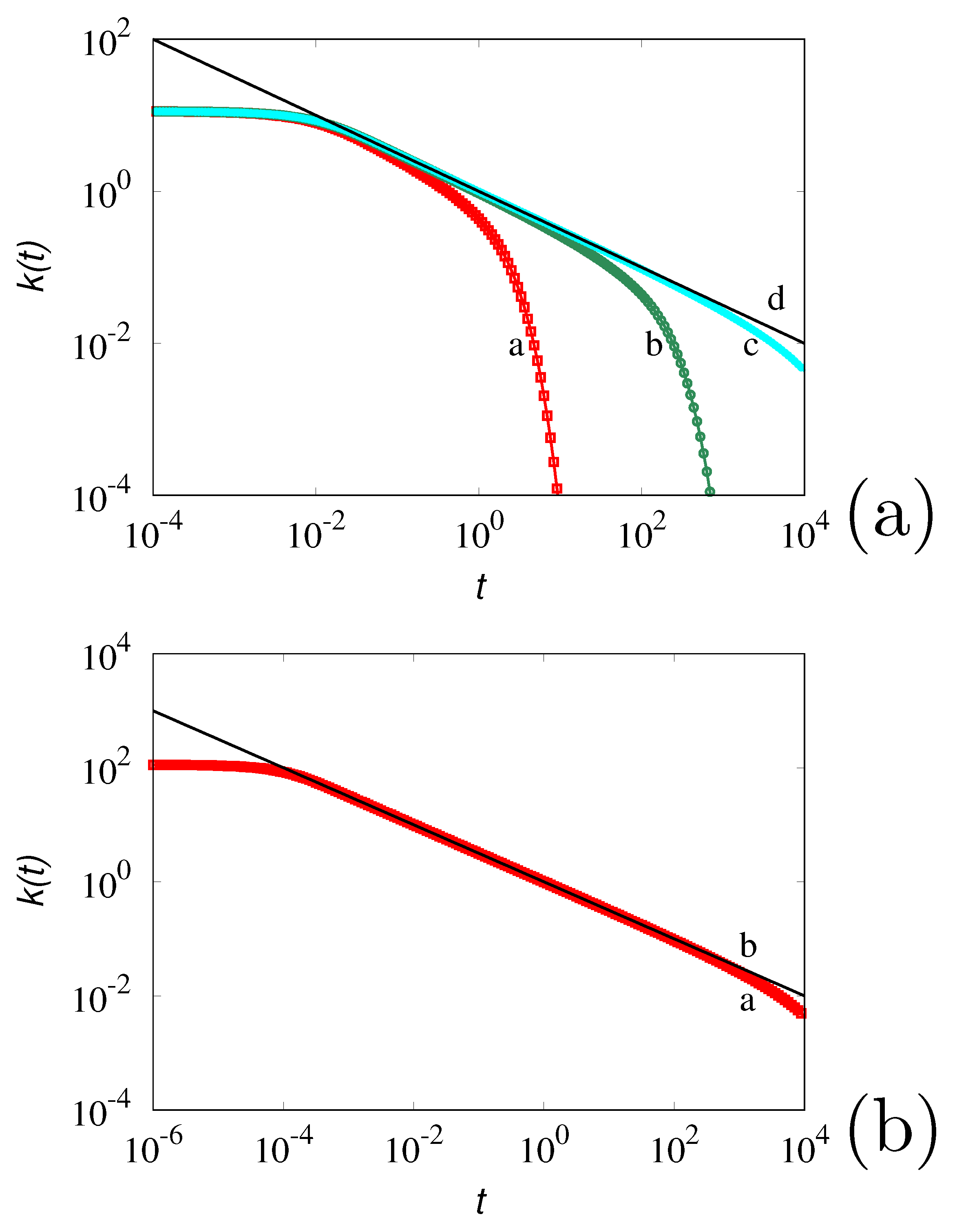
3.2. A Numerical Case Study

Let us consider the modal expansion in Equations (20)–(22) and its discretization with respect to k. Let $k_{\max }$ be the maximum value of k considered, and $\Delta k$ the step size in the discretization. Assuming $q=2/\sqrt{\pi }$, for the sake of normalization, the expression for $k_k\left(t\right)$ becomes

$$k_k\left(t\right)=\frac{2\Delta k}{\sqrt{\pi }}\sum _{i=1}^N{e}^{-{(i\Delta k)}^{2}t}$$

(34)

where $N=[k_{\max }/\Delta k]$ and $\left[x\right]$ represents the closest integer to the real-valued x. In the limit for $\Delta k\to 0$, and $k_{\max }\to \infty$, $k_k\left(t\right)$ defined by Equation (34) converges to $k_{\infty }\left(t\right)=1/\sqrt{t}$. Figure 1a depicts the behavior of the discretized $k_k\left(t\right)$ at $k_{\max }=10$ for decreasing values of $\Delta k$. As expected, as $\Delta k$ decreases to zero, the deviations of $k_k\left(t\right)$ from $k_{\infty }\left(t\right)$ become negligible for $t>1/k_{\max }^2$.

Similarly, the value of $k_{\max }$ controls the convergence to $k_{\infty }\left(t\right)$ at short time scales. Figure 1b depicts the behavior of $k_k\left(t\right)$ at $k_{\max }=100$, $\Delta k=0.01$. An accurate representation for $k_{\infty }\left(t\right)$ is achieved for $t>{10}^{-4}$. The analysis of these data indicates that $k_{\max }$ controls the behavior of $k_k\left(t\right)$ near $t=0$, which reaches a finite limiting value $k\left(0\right)\simeq k_{\mathrm{kmax}}$. This property seems to be a basic limitation of any discretization of the Basset force. In point of fact, as shown in the next section, the occurrence of a bounded value of $k_k\left(0\right)$ is a physical constraint derived from the viscoelastic nature of a liquid phase. And all the fluid, including water at room temperature, possesses a characteristic non vanishing relaxation time.

Consider Equation (10) for a macroscopic particle (radius greater than a millimeter or higher), for which the stochastic fluctuations could be neglected. Substituting on it the modal expansion Equation (34), we have

$$\begin{array}{ccc}\hfill m_e\frac{d{\mathbf{V}}_p\left(t\right)}{dt}& =& -\eta {\mathbf{V}}_p\left(t\right)-\frac{2\beta \Delta k}{\sqrt{\pi }}\sum _{i=1}^N{e}^{-{(i\Delta k)}^{2}t}\ast \left(\frac{d{\mathbf{V}}_p\left(t\right)}{dt}+V_p\left(0\right)\delta \left(t\right)\right)\hfill \\ & =& -\eta {\mathbf{V}}_p\left(t\right)-\frac{2\beta \Delta k}{\sqrt{\pi }}\sum _{i=1}^N{\mathbf{z}}_i\left(t\right)\hfill \end{array}$$

(35)

where $\beta =6\sqrt{\pi \rho \mu }{R}^2$, as it stems from Equation (9), and ${\mathbf{z}}_i\left(t\right)$, $i=1,\cdots ,N$ is a system of N auxiliary degrees of freedom accounting for fluid inertial effects, the equations for which read

$$\begin{array}{ccc}\hfill \frac{d{\mathbf{z}}_i\left(t\right)}{dt}& =& -{\mu }_i{\mathbf{z}}_i\left(t\right)+\frac{d{\mathbf{V}}_p\left(t\right)}{dt}\hfill \\ & =& -\left({\mu }_i+\eta \right){\mathbf{z}}_i\left(t\right)-\frac{2\beta \Delta k}{\sqrt{\pi }}\sum _{i=1}^N{\mathbf{z}}_i\left(t\right)\hfill \end{array}$$

(36)

where ${\mu }_i={(i\Delta k)}^2$, and the impulsive initial contribution has been included into the initial condition for ${\mathbf{z}}_i\left(0\right)={\mathbf{V}}_p\left(0\right)$.

Equation (35) represents a major advantage of the model expansion compared to the more recent computational approaches for addressing inertial particle motion [47], as it reduces the integro-differential particle equations of motion to a system of ordinary differential equations that can be solved using standard numerical routines. The analysis here presented for a quiescent fluid can be straightforwardly extended to the presence of a macroscopic (e.g., pressure-driven) velocity field in the fluid phase.

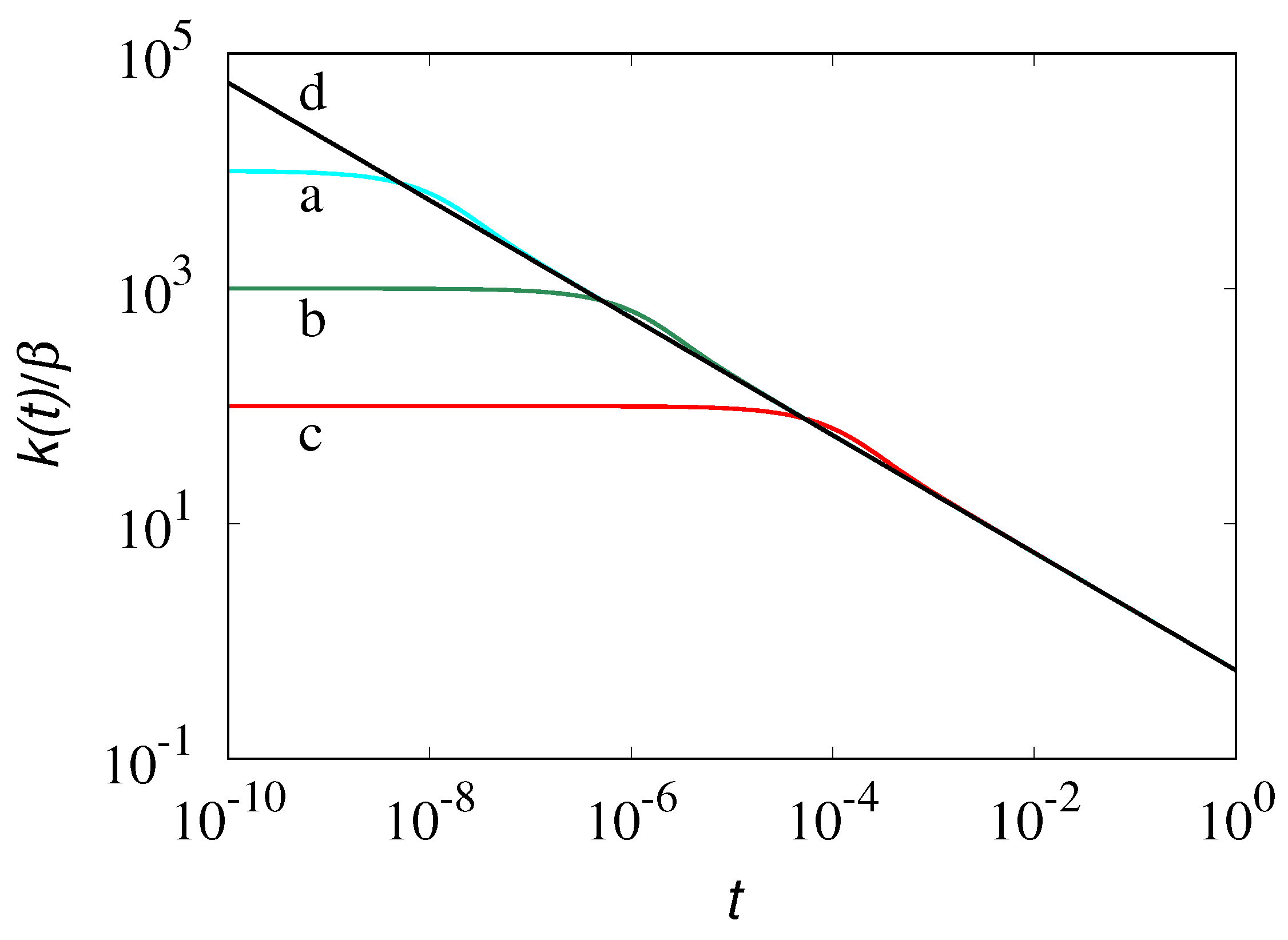
4. Regularity of Inertial Kernels

The second main issue addressed in this article concerns the regularity of the inertial memory kernels $k\left(t\right)$, once basic physical requirements (such as the bounded propagation of any physical phenomenon, limited by the speed of light vacuo, as a consequence of relativity theory) are taken into account. We have seen in Section 2 that the Basset kernel diverges at $t=0$, as seen in Equation (9). As explained below, this is a consequence of the infinite propagation velocity of the internal stresses that characterize the Newtonian constitutive Equation (5). This phenomenon is altogether analogous to the divergence of interfacial fluxes in heat/mass transfer parabolic problems in the presence of a discontinuity between the initial and the boundary conditions at a boundary. This problem can be resolved by removing the paradox of infinite propagation velocity intrinsic to any Fickian/Fourier constitutive equation, simply considering the hyperbolic extension of the transport problem [52].

In the hydrodynamic case, the corresponding hyperbolic generalization merely consists in accounting for fluid viscoelasticity, which is a generic property of any liquid phases. In point of fact, even water at ambient conditions (temperature $T=300$ K, pressure $p={10}^5$ Pa) behaves as a viscoelastic fluid, but its characteristic relaxation time, ${\theta }^c\simeq 1$ ps [53,54], is so small that it can be neglected in the overwhelming majority of hydrodynamic problems, since the observation time scales in most of the practical cases of interest are widely larger than ${\theta }^c$.

To begin with, let us consider the case of a viscoelastic fluid characterized by a single relaxation time ${\theta }^c$ (Maxwell fluid). Neglecting the nonlinear terms in the objective definition of the viscoelastic constitutive equation involving the Oldroyd upper convective derivative [33] (which are small for the typical conditions of Brownian and micrometric particles in microchannels), Equation (5) is replaced by the following viscoelastic constitutive equation:

$${\theta }^c\frac{\partial \mathbf{\tau }}{\partial t}+\mathbf{\tau }=-\mu \left(\nabla \mathbf{v}+\nabla {\mathbf{v}}^T\right)$$

(37)

that in the Laplace domain takes the following simple expression:

$$\widehat{\mathbf{\tau }}(\mathbf{x},s)=-{\widehat{\mu }}_e\left(s\right)\left[\nabla \widehat{\mathbf{v}}(\mathbf{x},s)+\nabla \widehat{\mathbf{v}}{(\mathbf{x},s)}^T\right]$$

(38)

where

$${\widehat{\mu }}_e\left(s\right)=\frac{\mu }{{\theta }^c(s+1/{\theta }^c)}$$

(39)

Consequently, the Laplace transform of ${\widehat{\mathbf{F}}}_{f\to p}\left(s\right)$ of the force subjected by the particle is still given by Equation (7), with the constant viscosity $\mu$ replaced by the function ${\widehat{\mu }}_e\left(s\right)$. As well known, this modifies the instantaneous dissipative Stokesian friction ${\mathbf{F}}_{f\to p}^{\left(d\right)}\left[{\mathbf{V}}_p\left(t\right)\right]=-\eta {\mathbf{V}}_p\left(t\right)$ into a memory term

$${\mathbf{F}}_{f\to p}^{\left(d\right)}\left[{\mathbf{V}}_p\left(t\right)\right]=-\eta \frac{1}{{\theta }^c}{\int }_0^t{e}^{-(t-\tau )/{\theta }^c}{\mathbf{V}}_p\left(\tau \right)d\tau$$

(40)

while the inertial Basset term attains in the Laplace domain the form $-\widehat{k}\left(s\right)s{\widehat{\mathbf{V}}}_p\left(s\right)$ with

$$\widehat{k}\left(s\right)=\frac{\beta }{\sqrt{{\theta }^c}}\frac{1}{\sqrt{s(s+1/{\theta }^c)}}$$

(41)

where $\beta =6\pi \sqrt{\rho \mu }{R}^2$. It is easy to see that the presence of a non-vanishing relaxation time ${\theta }^c>0$ determines a finite value of $k\left(t\right)$ for $t=0$. Enforcing the initial value theorem of Laplace transforms, we have from Equation (41)

$$\underset{t\to 0}{lim}k\left(t\right)=\underset{s\to \infty }{lim}s\widehat{k}\left(s\right)=\frac{\beta }{\sqrt{{\theta }^c}}$$

(42)

In point of fact, the inverse Laplace transform of $\widehat{k}\left(s\right)$ is given by

$$k\left(t\right)=\frac{\beta }{\sqrt{{\theta }^c}}{e}^{-t/2{\theta }^c}{I}_0\left(\frac{t}{2{\theta }^c}\right)$$

(43)

where $I_0\left(\xi \right)$ is the modified Bessel function of the first kind, which possesses the following asymptotic behaviors:

$$I_0\left(0\right)=1,I_0\left(\xi \right)=\frac{e^{\xi }}{\sqrt{2\pi \xi }}\left[1+O\left(\frac{1}{\xi }\right)\right]$$

(44)

From Equation (44), the asymptotics of the Newtonian Basset kernel is recovered for $t\gg {\theta }^c$. This phenomenon is depicted in Figure 2 for several values of ${\theta }^c$. The viscoelastic kernel practically coincides with the Basset counterpart of a Newtonian fluid for $t>5{\theta }_c$.

The occurrence of a finite value for $k\left(0\right)$ has been observed in Newtonian fluids once slip boundary conditions are enforced at the surface of the solid particle [55,56,57]. The physical reason for this occurrence, and the eventual analogy with the viscoelastic case, is still an open question.

4.1. Field-Theoretical Analysis

The result expressed by Equation (43) can be recovered from the field approach addressed in the previous section. The presence of viscoelastic effects characterized by a single relaxation time ${\theta }^c$ implies to substitute the parabolic diffusion model Equation (28) with the hyperbolic Cattaneo equation

$$\rho {\theta }^c\frac{{\partial }^{2}v(x,t)}{\partial t^2}+\rho \frac{\partial v(x,t)}{\partial t}=\mu \frac{{\partial }^{2}v(x,t)}{\partial x^2}+f(x,t)$$

(45)

while $f(x,t)$ is identical to Equation (29). The solution of this impulsive model, with ${v(x,0)=\partial v(x,t)/\partial t|}_{t=0}=0$, takes the following form (see [58], p. 320):

$$v(x,t)=\frac{1}{2}\sqrt{\frac{\rho {\theta }^c}{\mu }}\frac{D}{{\theta }_c}{\int }_0^t{e}^{-(t-\tau )/2{\theta }^c}{I}_0\left(\frac{1}{2{\theta }^c}\sqrt{{(t-\tau )}^2-{(x-x_c)}^2\rho {\theta }^c/\mu }\right)\frac{d{V}_p\left(\tau \right)}{d\tau }d\tau$$

(46)

that for $x=x_c$, and $t\ge \tau$ reduces to

$$v_c\left(t\right)=\frac{1}{2}\sqrt{\frac{\rho }{\mu {\theta }^c}}D{\int }_0^t{e}^{-(t-\tau )/2{\theta }^c}{I}_0\left(\frac{t-\tau }{2{\theta }^c}\right)\frac{d{V}_p\left(\tau \right)}{d\tau }d\tau$$

(47)

providing the same expression for $k\left(t\right)$ derived above, as seen in Equation (43).

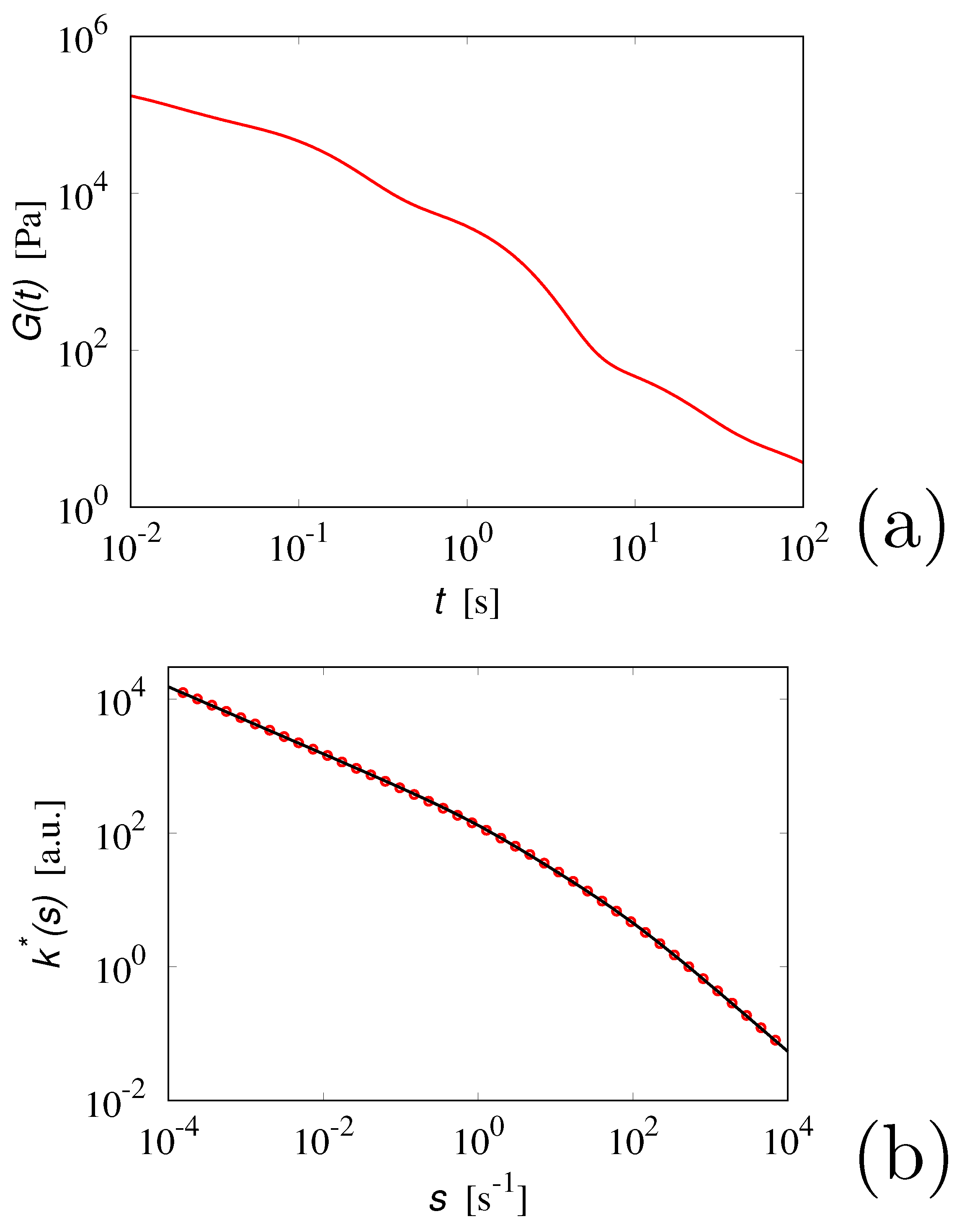
4.2. Extension to Complex Fluids

The analysis developed above for a viscoelastic fluid possessing a single relaxation time can be generalized to more complex and real fluids. The problem can be stated as follows. Consider a real fluid and suppose to have obtained from rheological experiments the functional form of the dissipation memory kernel $G\left(t\right)$ entering the expression of the dissipative contribution to the force exerted by the fluid on a spherical particle

$${\mathbf{F}}_{f\to p}^{\left(d\right)}\left[{\mathbf{V}}_p\left(t\right)\right]=-6\pi R{\int }_0^{t}G(t-\tau ){\mathbf{V}}_p\left(\tau \right)d\tau$$

(48)

Does this information provide a way to quantify the inertial contribution, and specifically the expression for the generalized Basset force in this fluid?

This problem can be tackled as follows. The convolutional nature of Equation (48) suggests that the constitutive equation for the shear stresses is of the form

$$L_t\left[\mathbf{\tau }\right]=-\mu \left(\nabla \mathbf{v}+\nabla {\mathbf{v}}^T\right)$$

(49)

where $L_t$ is a linear operator acting on the stress tensor $\mathbf{\tau }$, and containing its derivatives of any order n, $n=0,1,\dots$, with respect to time, and eventually also its fractional time derivatives (Riemann–Liouville operators) [59]. In the Laplace domain, Equation (49) becomes

$$\widehat{\ell }\left(s\right)\widehat{\mathbf{\tau }}(\mathbf{x},s)=-\mu \left[\nabla \widehat{\mathbf{v}}(\mathbf{x},s)+\nabla \widehat{\mathbf{v}}{(\mathbf{x},s)}^T\right]$$

(50)

where $\widehat{\ell }\left(s\right)$ is a function of the Laplace variable s. Equation (50) coincides with Equation (38), and ${\widehat{\mu }}_e\left(s\right)$, coinciding with $\widehat{G}\left(s\right)$, is now expressed by

$${\widehat{\mu }}_e\left(s\right)=\frac{\mu }{\widehat{\ell }\left(s\right)}=\widehat{G}\left(s\right)$$

(51)

The analysis developed above for a Maxwell fluid can be applied to this more general problem, providing for the Laplace transform of the inertial memory kernel the following expression:

$$\widehat{k}\left(s\right)=6\sqrt{\rho }{R}^2\sqrt{\frac{\widehat{G}\left(s\right)}{s}}$$

(52)

The inverse Laplace transform $k\left(t\right)$ of $\widehat{k}\left(s\right)$ defined by Equation (52) cannot be obtained analytically for generic $\widehat{G}\left(s\right)$. Nevertheless, it is always possible to derive accurate representations for $k\left(t\right)$ enforcing Equation (52).

In order to make a practical example, consider the rheological data for polydimethilsiloxane at $T=25$ °C reported in [33], for which an accurate representation involves the occurrence of $N=5$ relaxation rates ${\lambda }_h$, $h=1,\dots ,N$,

$$G\left(t\right)=\sum _{h=1}^N{a}_h{e}^{-{\lambda }_{h}t}$$

(53)

where ${\lambda }_h=1/{\theta }_h^c$, $h=1,\dots ,N$ are the relaxation rates i.e., the reciprocal of the relaxation times ${\theta }_h^c$. The values for ${\lambda }_h$ and for the expansion coefficients $a_h$ can be found in [33] (p. 114), and the graph of the resulting $G\left(t\right)$ is depicted in Figure 3a. Applying Equation (52) to this case we obtain

$$\widehat{k}\left(s\right)=\alpha \sqrt{\frac{1}{s}\sum _{h=1}^N\frac{a_h}{s+{\lambda }_h}},\alpha =6\pi \sqrt{\rho }{R}^2$$

(54)

The graph of $k^{*}\left(s\right)=\widehat{k}\left(s\right)/\alpha$ is depicted in Figure 3b (symbols). The data can be accurately approximated over the time scales of interest by a linear combination of the inertial contributions obtained for the simple Maxwell fluid Equation (41), each of which is characterized by a different relaxation time

$$k^{*}\left(s\right)=\sum _{h=1}^{N_i}\frac{c_h}{\sqrt{s(s+b_h)}}$$

(55)

Making use of Equation (43), the memory inertial kernel $k\left(t\right)$ is given in this case by the expression

$$k\left(t\right)=\alpha \sum _{h=1}^{N_i}{c}_h{e}^{-b_{h}t/2}{I}_0\left(\frac{b_{h}t}{2}\right)$$

(56)

For the use made above of the solutions obtained for the simple Maxwell fluid, each term of the form (41) in the Laplace domain, and (43) in the time domain, can be referred to as a “prototypical visco-inertial mode”. In the present case, it is sufficient to consider the combination of $N_i=2$ prototypical visco-inertial modes, and the resulting approximation is depicted in Figure 3b. The values of the parameters are $c_1=125$ a.u., $b_1=1.52$ s⁻¹, $c_2=420$ a.u., $b_2=65$ s⁻¹. The corresponding inertial memory kernel $k\left(t\right)$, i.e., the graph of Equation (56), is depicted in Figure 4.

From this practical example, we can draw the following conclusions:

• Enforcing the constitutive model Equation (49), corresponding to the rheological description of a complex viscoelastic fluid, it is possible to derive the functional form of the fluid inertial kernel $k\left(t\right)$ from rheological data, i.e., from the functional form of $G\left(t\right)$;
• The fluid inertial kernel $k\left(t\right)$ can be expressed as linear combination of a few prototypical visco-inertial modes;
• The number $N_i$ of modes required to provide an accurate representation of $k\left(t\right)$ does not necessarily coincide with the number N of dissipative (exponential) modes adopted for reconstructing $G\left(t\right)$.

Of course, it is possible to provide alternative representations of $k\left(t\right)$, e.g., adopting the modal decomposition discussed in Section 3. While for an accurate representation of the classical Basset kernel, a uncountable system of exponentially decaying modes is required, the physical constraint of bounded $k\left(t\right)$ permits to achieve accurate approximation for $k\left(t\right)$ using a finite (and relatively small) number of exponentially decaying modes.

4.3. Toward a Comprehensive Theory of Brownian Motion

To conclude, we can frame another central issue that takes advantage of the present theory. For a microparticle in a quiescent fluid (Brownian particle), the equations of motions in a real complex fluid, accounting for viscoelastic dissipation, fluid inertial effects and thermal fluctuations can be expressed in the form

$$m_e\frac{d{\mathbf{V}}_p\left(t\right)}{dt}=-h\left(t\right)\ast {\mathbf{V}}_p\left(t\right)-k\left(t\right)\ast \left(\frac{d{\mathbf{V}}_p\left(t\right)}{dt}+{\mathbf{V}}_p\left(0\right)\delta \left(t\right)\right)+\mathbf{S}\left(t\right)$$

(57)

where $h\left(t\right)$ is the viscoelastic kernel proportional to $G\left(t\right)$ defined by the linear functional form Equation (53), and $k\left(t\right)$ is the corresponding fluid inertial kernel, the properties of which have been addressed in the previous section. From rheological data, the viscoelastic kernel can be expressed as a linear combination of N modes, where usually $N<10$ for most of the fluids [33], i.e., $h\left(t\right)={\sum }_{j=1}^N{h}_j{e}^{-{\lambda }_{j}t}$. In a similar way, the fluid inertial kernel $k\left(t\right)$ analyzed in the previous section can also be accurately approximated by means of a system of exponentially decaying modes,

$$k\left(t\right)\simeq \sum _{i=1}^{N_i}{k}_i{e}^{-{\mu }_{i}t}$$

(58)

where the rates ${\mu }_i>0$, $i=1,\dots ,N_i$, are in general not related to the relaxation rates ${\lambda }_j$, $j=1,\dots ,N$ and $N_i\gg N$. The property that $k\left(0\right)$ is bounded ensures, as discussed in the previous section, that the approximation Equation (58) can be arbitrarily accurate in the metrics of continuous functions. This means that for any $\epsilon >0$, there exist a finite $N_i$, and finite rates ${\mu }_i>0$, $i=1,\dots ,N_i$, such that $\left|k\left(t\right)-{\sum }_{i=1}^{N_i}{k}_i{e}^{-{\mu }_{i}t}\right|<\epsilon$ for any $t\ge 0$. Consequently, Equations (57) reduce to the form

$$\begin{array}{ccc}\hfill m_e\frac{d{\mathbf{V}}_p\left(t\right)}{dt}& =& -\sum _{j=1}^N{h}_j{e}^{-{\lambda }_{j}t}\ast {\mathbf{V}}_p\left(t\right)-\sum _{i=1}^{N_i}{k}_i{e}^{-{\mu }_{i}t}\ast \left(\frac{d{\mathbf{V}}_p\left(t\right)}{dt}+{\mathbf{V}}_p\left(0\right)\delta \left(t\right)\right)+\mathbf{S}\left(t\right)\hfill \end{array}$$

(59)

In order to solve these stochastic differential equations, the expression for $\mathbf{S}\left(t\right)$ should be determined, and it would constitute the generalization of the celebrated Kubo fluctuation–dissipation theorem of the second kind [32,37], of which the original formulation is restricted to the pure dissipative case (i.e., to $k\left(t\right)=0$). The analysis of this problem is beyond the scope of this article and it will be addressed in a forthcoming work [60]. It can however be anticipated that the occurrence of a finite value of $k\left(0\right)$, coupled with the modal expansion of the memory kernels ($h\left(t\right)$ and $k\left(t\right)$) provide the key physical and formal ingredients toward an elegant solution of this problem.

5. Concluding Remarks

This article has presented a comprehensive description of the mathematical properties of the fluid inertial kernel entering the particle equation of motion in a complex viscoelastic fluid. Two main conclusions can be drawn from the present analysis and results. The modal expansion addressed in Section 3 naturally leads to a simplified field-theoretical representation of the fluid inertial effects. The latter has been successfully applied to non-trivial cases, such as a Maxwell fluid, in order to relate the disappearance of the $k\left(t\right)$-singularity at $t=0$ with the physics of stress propagation. It is noteworthy that a simple one-dimensional field-theoretical description could capture the inertial fluid–particle interactions in isotropic conditions (free space). This point deserves further investigation.

The boundedness of $k\left(0\right)$ is indeed a consequence of the finite propagation velocity of the internal shear stresses, and this is in agreement with fundamental physical principles (special relativity theory). The importance of this result is that the regularity of the fluid inertial kernel has been derived from physical principles, and not as the result of ad hoc mathematical regularization/mollification techniques. In rheological modeling, this simply corresponds to the occurrence of a viscoelastic constitutive model with non-vanishing relaxation times. For the sake of clarity, the inclusion of viscoelasticity does not ensure either that the corresponding hydrodynamic model is Lorentz covariant [61] nor that all the hydrodynamic perturbations (for instance, density and pressure waves) would propagate at finite speed. In order to match the latter condition, the occurrence of acoustic modes should be included in the description of hydromechanical phenomena as discussed in [8].

The case of a Maxwell fluid, characterized by a single relaxation time, not only provides an analytic expression for the fluid inertial kernel $k\left(t\right)$, but it represents the prototypical model for expressing the fluid inertial effects of more complex fluids. The representation of $\widehat{k}\left(s\right)$ starting from rheological data on the dissipation kernel $G\left(t\right)$ is a simple but relevant result, which applies to any complex fluids.

We have considered in this article spherical micrometric particles, but the obtained results are independent of the geometry of the particles and of the flow domain. Consequently, these results can be extended to particles of arbitrary shape, and to confined geometries of flow devices, provided that the parameters controlling the expression for the force acting on the particle (attaining a tensorial character [5,49]) are known in the case of a Newtonian fluid.

The results obtained in this article are also propedeutical for addressing and solving the other crucial problem associated with micrometric particle motion mentioned in Section 2 and Section 4.3, namely the determination of an analytical representation for the stochastic force $\mathbf{S}\left(t\right)$ at thermal equilibrium in the presence of fluid inertial effects. This represents, in the terminology introduced by Kubo [32,37], the fluctuation–dissipation relation of the second kind (see [32], p. 37 and the discussion therein), in the presence of fluid inertial effects. This topic is outside the scope of the present article and it will be addressed elsewhere [60]. Nevertheless, it is important to mention that the key ingredient for an elegant solution of this problem is represented by the boundedness of the fluid inertial kernel $k\left(t\right)$, proved in the present work for viscoelastic fluids. This could lead to an entropic characterization of the dissipation effects deriving from rheological/inertial properties of complex fluids into which a diffusing Brownian particle is immersed and moves under constant temperature conditions.

References

1. Sackmann, E.K.; Fulton, A.L.; Beebe, D.J. The present and future role of microfluidics in biomedical research. Nature 2014, 507, 181–189. [Google Scholar] [CrossRef] [PubMed]
2. Guazzelli, E.; Morris, J.F. A Physical Introduction to Suspension Dynamics; Cambridge University Press: Cambridge, UK, 2012. [Google Scholar]
3. Brenner, H.; Ganesan, V. Molecular wall effects: Are conditions at a boundary “boundary conditions”? Phys. Rev. E 2000, 61, 6879. [Google Scholar] [CrossRef] [PubMed]
4. Ho, B.P.; Leal, L. Inertial migration of rigid spheres in two-dimensional unidirectional flows. J. Fluid Mech. 1974, 65, 365–400. [Google Scholar] [CrossRef]
5. Procopio, G.; Giona, M. Stochastic Modeling of Particle Transport in Confined Geometries: Problems and Peculiarities. Fluids 2022, 7, 105. [Google Scholar] [CrossRef]
6. Zwanzig, R.; Bixon, M. Compressibility effects in the hydrodynamic theory of Brownian motion. J. Fluid Mech. 1975, 69, 21–25. [Google Scholar] [CrossRef]
7. Chow, T.S.; Hermans, J.J. Brownian motion of a spherical particle in a compressible fluid. Physica 1973, 65, 156–162. [Google Scholar] [CrossRef]
8. Giona, M.; Procopio, G.; Adrover, A.; Mauri, R. New formulation of the Navier–Stokes equations for liquid flows. J. Non-Equilib. Thermodyn. 2022. [Google Scholar] [CrossRef]
9. Lauga, E.; Brenner, M.; Stone, H. Microfluidics: The No-Slip Boundary Condition. In Springer Handbook of Experimental Fluid Mechanics; Tropea, C., Yarin, A.L., Foss, J.F., Eds.; Springer: Berlin/Heidelberg, Germany, 2007; pp. 1219–1240. [Google Scholar]
10. Lauga, E.; Squires, T.M. Brownian motion near a partial-slip boundary: A local probe of the no-slip condition. Phys. Fluids 2005, 17, 103102. [Google Scholar] [CrossRef] [Green Version]
11. Mo, J.; Simha, A.; Raizen, M.G. Brownian motion as a new probe of wettability. J. Chem. Phys. 2017, 146, 134707. [Google Scholar] [CrossRef] [Green Version]
12. Giona, M.; Brasiello, A.; Crescitelli, S. Stochastic foundations of undulatory transport phenomena: Generalized Poisson–Kac processes—Part III extensions and applications to kinetic theory and transport. J. Phys. A 2017, 50, 335004. [Google Scholar] [CrossRef] [Green Version]
13. Einstein, A. Investigations on the Theory of Brownian Movement; Dover Publ.: Mineola, NY, USA, 1956. [Google Scholar]
14. Langevin, P. Sur la theorie du mouvement brownien. C. R. Acad. Sci. 1908, 146, 530–533. [Google Scholar]
15. Cichocki, B. (Ed.) Marian Smoluchowski—Selected Scientific Works; WUW: Warsaw, Poland, 2017. [Google Scholar]
16. Chandrasekhar, S. Stochastic problems in physics and astrophysics. Rev. Mod. Phys. 1943, 15, 1–89. [Google Scholar] [CrossRef]
17. Frey, E.; Kroy, K. Brownian motion: A paradigm of soft matter and biological physics. Ann. Der Phys. 2005, 517, 20–50. [Google Scholar] [CrossRef]
18. Bian, X.; Kim, C.; Karniadakis, G.E. 111 years of Brownian motion. Soft Matter 2016, 12, 6331–6346. [Google Scholar] [CrossRef] [Green Version]
19. Mo, J.; Raizen, M.G. Highly resolved Brownian motion in space and in time. Annu. Rev. Fluid Mech. 2019, 51, 403–428. [Google Scholar] [CrossRef]
20. Raizen, M.G.; Li, T. The measurement Einstein deemed impossible. Phys. Today 2016, 68, 56–57. [Google Scholar] [CrossRef]
21. Huang, R.; Chavez, I.; Taute, K.M.; Lukic, B.; Jeney, S.; Raizen, M.G.; Florin, E.L. Direct observation of the full transition from ballistic to diffusive Brownian motion in a liquid. Nat. Phys. 2011, 7, 576–580. [Google Scholar] [CrossRef]
22. Franosch, T.; Grimm, M.; Belushkin, M.; Mor, F.M.; Foffi, G.; Forró, L.; Jeney, S. Resonances arising from hydrodynamic memory in Brownian motion. Nature 2011, 478, 85–88. [Google Scholar] [CrossRef]
23. Pusey, P.N. Brownian motion goes ballistic. Science 2011, 332, 802–803. [Google Scholar] [CrossRef]
24. Kheifets, S.; Simha, A.; Melin, K.; Li, T.; Raizen, M.G. Observation of Brownian motion in liquids at short times: Instantaneous velocity and memory loss. Science 2014, 343, 1493–1496. [Google Scholar] [CrossRef]
25. Grimm, M.; Jeney, S.; Franosch, T. Brownian motion in a Maxwell fluid. Soft Matter 2011, 7, 2076–2084. [Google Scholar] [CrossRef] [Green Version]
26. Zwanzig, R.; Bixon, M. Hydrodynamic theory of the velocity correlation function. Phys. Rev. A 1970, 2, 2005. [Google Scholar] [CrossRef]
27. Widom, A. Velocity fluctuations of a hard-core Brownian particle. Phys. Rev. A 1971, 3, 1394. [Google Scholar] [CrossRef]
28. Burgess, R.E. Brownian motion and the equipartition theorem. Phys. Lett. A 1973, 42, 395–396. [Google Scholar] [CrossRef]
29. Mo, J.; Simha, A.; Kheifets, S.; Raizen, M.G. Testing the Maxwell-Boltzmann distribution using Brownian particles. Opt. Express 2015, 23, 1888–1893. [Google Scholar] [CrossRef] [PubMed] [Green Version]
30. Darwin, C. Note on hydrodynamics. Math. Proc. Camb. Phil. Soc. 1953, 49, 342–354. [Google Scholar] [CrossRef]
31. Landau, L.D.; Lifshitz, E.M. Fluid Mechanics; Pergamon Press: Oxford, UK, 1993. [Google Scholar]
32. Kubo, R.; Toda, M.; Hashitsume, N. Statistical Physics II—Nonequilibrium Statistical Mechanics; Springer: Berlin/Heidelberg, Germany, 1991. [Google Scholar]
33. Makosko, C.W. Rheology—Principles, Measurements, and Applications; Wiley-VCH: New York, NY, USA, 1994. [Google Scholar]
34. Zwanzig, R. Memory Effects in Irreversible Thermodynamics. Phys. Rev. 1961, 124, 983–992. [Google Scholar] [CrossRef]
35. Mori, H. Transport, Collective Motion, and Brownian Motion. Prog. Theor. Phys. 1965, 33, 423–455. [Google Scholar] [CrossRef] [Green Version]
36. Zwanzig, R. Nonlinear Generalized Langevin Equations. J. Stat. Phys. 1973, 9, 215–220. [Google Scholar] [CrossRef]
37. Kubo, R. The fluctuation-dissipation theorem. Rep. Prog. Phys. 1966, 29, 255–284. [Google Scholar] [CrossRef] [Green Version]
38. Alder, B.J.; Wainwright, T.E. Decay of the Velocity Autocorrelation Function. Phys. Rev. A 1970, 1, 18–21. [Google Scholar] [CrossRef]
39. D’Avino, G.; Maffettone, P.L. Particle dynamics in viscoelastic liquids. Non-Newton. Fluid Mech. 2015, 215, 80–104. [Google Scholar] [CrossRef]
40. D’Avino, G.; Greco, F.; Maffettone, P.L. Particle Migration due to Viscoelasticity of the Suspending Liquid and Its Relevance in Microfluidic Devices. Annu. Rev. Fluid Mech. 2017, 49, 341–360. [Google Scholar] [CrossRef]
41. Segré, S.; Silberberg, A. Radial particle displacements in Poiseuille flow of suspensions. Nature 1961, 189, 209–220. [Google Scholar] [CrossRef]
42. Ho, B.P.; Leal, L.G. Migration of rigid spheres in a two-dimensional unidirectional shear flow of a second-order fluid. J. Fluid Mech. 1976, 76, 783–799. [Google Scholar] [CrossRef] [Green Version]
43. Provencher-Langlois, G.; Farazmand, M.; Haller, G. Asymptotic dynamics of inertial particles with memory. J. Nonlinear Sci. 2015, 25, 1225–1255. [Google Scholar] [CrossRef] [Green Version]
44. Parmar, M.; Annamalai, S.; Balachandar, S.; Prosperetti, A. Differential formulation of the viscous history force on a particle for efficient and accurate computation. J. Fluid Mech. 2018, 844, 970–993. [Google Scholar] [CrossRef] [Green Version]
45. Prasath, S.G.; Vasan, V.; Govindarajan, R. Accurate solution method for the Maxey–Riley equation, and the effects of Basset history. J. Fluid Mech. 2019, 868, 428–460. [Google Scholar] [CrossRef] [Green Version]
46. Maxey, M.R.; Riley, J.J. Equation of motion for a small rigid sphere in a nonuniform flow. Phys. Fluids 1983, 26, 883–889. [Google Scholar] [CrossRef]
47. Haller, G. Solving the inertial particle equation with memory. J. Fluid Mech. 2019, 874, 1–4. [Google Scholar] [CrossRef] [Green Version]
48. Kim, S.; Karrila, S.J. Microhydrodynamics—Principles and Selected Applications; Dover Publ.: Mineola, NY, USA, 2005. [Google Scholar]
49. Happel, J.; Brenner, H. Low Reynolds Number Hydrodynamics: With Special Applications to Particulate Media; Martinus Nijhoff: The Hague, The Netherlands, 1983. [Google Scholar]
50. Mazur, P.; Bedeaux, D. Causality, time-reversal invariance and the Langevin equation. Phys. A 1991, 173, 155–174. [Google Scholar] [CrossRef]
51. Bedeaux, D.; Mazur, P. Brownian motion and fluctuating hydrodynamics. Physica 1974, 76, 247–258. [Google Scholar] [CrossRef]
52. Giona, M. Generalized Poisson-Kac Processes and the regularity of laws of nature. Acta Phys. Pol. B 2019, 49, 827–857. [Google Scholar] [CrossRef] [Green Version]
53. Cunsolo, A.; Ruocco, G.; Sette, F.; Masciovecchio, C.; Mermet, A.; Monaco, G.; Sampoli, M.; Verbeni, R. Experimental Determination of the Structural Relaxation in Liquid Water. Phys. Rev. Lett. 1999, 82, 775–778. [Google Scholar] [CrossRef]
54. O’Sullivan, T.J.; Kannam, S.K.; Chakraborty, D.; Todd, B.D.; Sader, J.E. Viscoelasticity of liquid water investigated using molecular dynamics simulations. Phys. Rev. Fluids 2019, 4, 123302. [Google Scholar] [CrossRef]
55. Gatignol, R. On the history term of Boussinesq–Basset when the viscous fluid slips on the particle. Comptes Rendus Mec. 2007, 335, 606–616. [Google Scholar] [CrossRef]
56. Premlata, A.R.; Wei, H.-H. The Basset problem with dynamic slip: Slip-induced memory effect and slip–stick transition. J. Fluid Mech. 2019, 866, 431–449. [Google Scholar] [CrossRef]
57. Premlata, A.R.; Wei, H.-H. Atypical non-Basset particle dynamics due to hydrodynamic slip. Phys. Fluids 2020, 32, 097109. [Google Scholar] [CrossRef]
58. Polyanin, A.D. Handbook of Linear Partial Differential Equations for Engineers and Scientists; Chapman & Hall/CRC: Boca Raton, FL, USA, 2002. [Google Scholar]
59. Oldham, K.J.; Spanier, J. The Fractional Calculus; Dover Publ.: Mineola, NY, USA, 2006. [Google Scholar]
60. Giona, M.; Procopio, G.; Klages, R. Relativistic Hydrodynamics; La Sapienza University: Roma, Italy, 2023; (manuscript in preparation). [Google Scholar]
61. Rezzola, O.; Zanotti, O. Relativistic Hydrodynamics; Oxford University Press: Oxford, UK, 2013. [Google Scholar]
Figure 1. Behavior of the discretized  k k ( t ) defined by Equation (34) for different discretizations. Panel (a) refers to  k max = 10 , lines and symbols (a) to (c) correspond to  Δ k = 1 , 0.1 , 0.01 , respectively. Line (d) represents  k ( t ) = 1 / t . Panel (b k max = 100 Δ k = 0.01 (line a), while line (b) depicts  k ( t ) .
Fluids 08 00084 g001
Figure 2. Rescaled inertial kernel  k ( t ) / β , Equation (41) vs. t for a simple Maxwell fluid, characterized by the relaxation time  θ c . Lines (a) to (c) refer to  θ c = 10 4 , 10 6 , 10 8 , respectively. Line (d) depicts the asymptotic nondimensional Basset curve,  k ( t ) / β = 1 / π t .
Fluids 08 00084 g002
Figure 3. Panel (a G ( t ) vs. t for polydimethilsiloxane at  T = 25   ° C . Panel (b) (symbols)  k * ( s ) = k ^ ( s ) / α vs. s for the same fluid, obtained from Equation (54). The solid line is the approximation of these data using  N i = 2 , prototypical visco-inertial modes, as discussed in the main text.
Fluids 08 00084 g003
Figure 4. k ( t ) / α (line a) obtained from Equation (56) with  N i = 2 modes. Line (b) corresponds to the long-term scaling  k ( t ) / α 1 / t .
Fluids 08 00084 g004
Disclaimer/Publisher’s Note: The statements, opinions and data contained in all publications are solely those of the individual author(s) and contributor(s) and not of MDPI and/or the editor(s). MDPI and/or the editor(s) disclaim responsibility for any injury to people or property resulting from any ideas, methods, instructions or products referred to in the content.