5.1. Test Case Setup and Evaluation Strategy
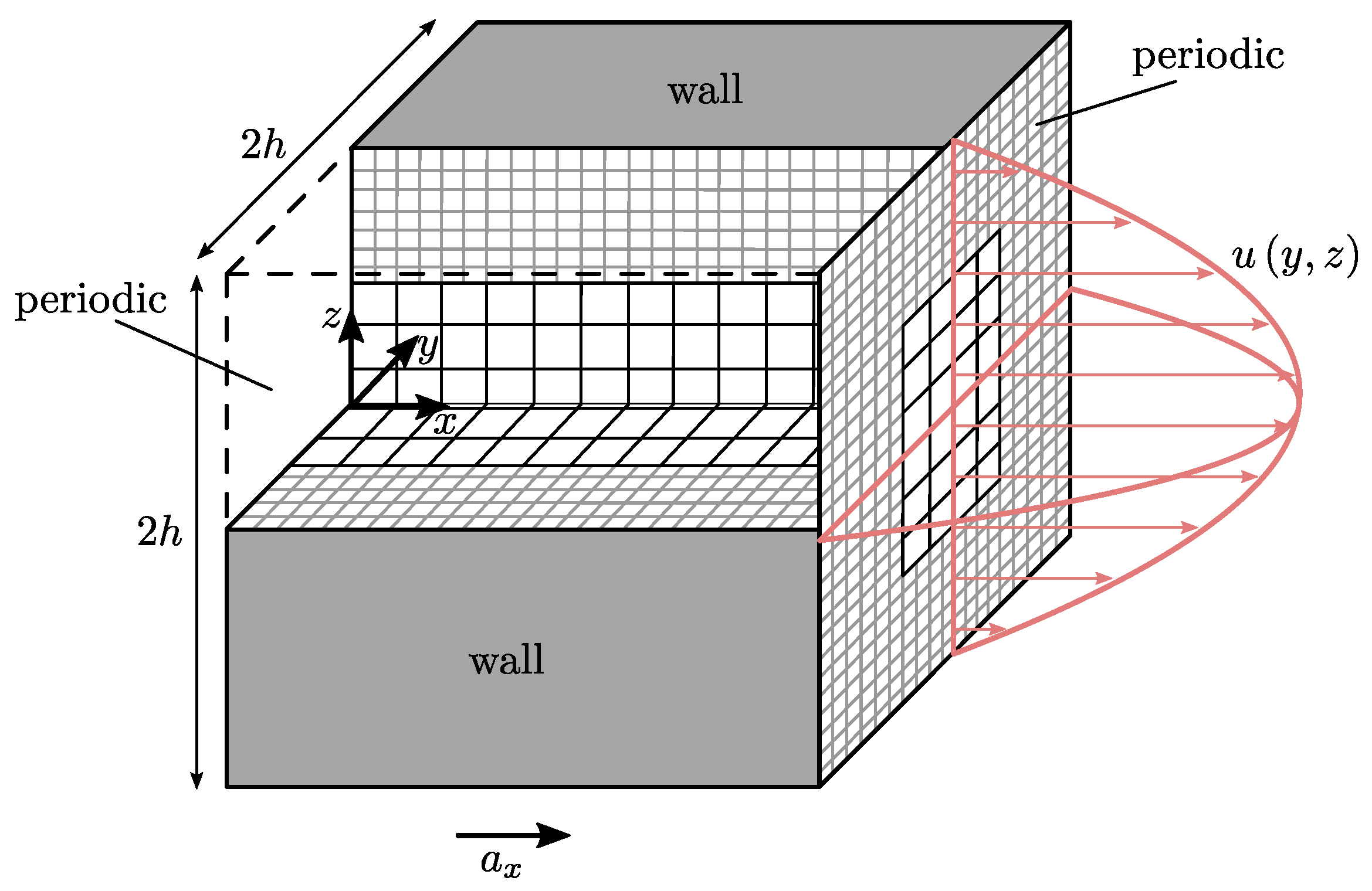
Numerical experiments for the stability evaluation of the grid transition algorithms and collision operators discussed in the previous chapters are performed using a force-driven square duct flow test case, schematically depicted in
Figure 9. Within subcritical Reynolds number regime, the analytical solution for the laminar velocity field is given by [
64]:
Here, is the kinematic viscosity and represents the uniform flow acceleration acting in positive x-direction, i.e., parallel to the duct center axis.
The simulations are performed in a periodic, cubic domain with characteristic width
, see
Figure 9. A single level reference case (abbr.
sl) with grid spacing
is used for comparison. In the multi-level case, the cubic domain is discretized using two levels of grid resolution
, with coarse cells located in the duct core and six refinement layers of fine cells at the surrounding duct walls, resulting in approximately
cells in total. This rather coarse grid resolution was chosen to keep the time frame for the numerical study within acceptable bounds. The grid transition interface with an overlap width of
for cell-vertex and cell-centered cases and an overlap width of
for the combined grid layout, is oriented parallel to the flow direction througout the complete domain. No-slip walls are implemented utilizing simple half-way bounce-back scheme, while periodic conditions enclose the domain at boundaries orthogonal to the flow direction. All simulations have been performed with the in-house lattice Boltzmann package SAM-Lattice.
As was shown by means of linear stability analysis for various collision models, the lattice Boltzmann method exhibits instabilities for high Reynolds number flows [
9,
10], which materialize in the form of physically meaningless negative values for the distribution functions
. As can be seen directly from the connection between dimensionless collision frequency and kinematic viscosity in Equation (
8), a Reynolds number tending towards infinity is associated with
. In order to examine the influence of the various grid transition schemes and collision models on accuracy and stability ranges for the square-duct flow, numerical experiments are performed. Through successive variation of the flow acceleration
, Reynolds number and consequently the collision frequency
are modified together with simultaneous verification of adherence to the following constraints, defining three distinct evaluation categories:
Category 1: Simulation remains stable, i.e.,
, and within the subcritical Reynolds number regime
[
65]
[
66]. Furthermore, iterative convergence
is reached with an averaged relative velocity error of
.
Category 2: Simulation remains stable, i.e., , but either averaged relative error increases to in subcritical regime or .
Category 3: Simulation is unstable and diverges, i.e., is detected.
Here, the Reynolds number
is based on the bulk velocity
and hydraulic equivalent diameter
for the square duct flow. The simulation parameters are summarized in
Table 1. Affiliation of a particular test case to one of these categories is expressed in terms of dimensionless collision frequency
, where superscript
c indicates a coarse grid value as before and subscript 1 or 2 represents the respective category. Regarding the first category, the procedure stops once the relative error increases to
in the subcritical regime and the condition for iterative convergence can no longer be met or
and thus a comparison with the analytical solution Equation (
62) is not permissible anymore. Consequently, in the remainder of this paper
represents the maximum value of
that just about satisfies these critera. As for the second category,
variation terminates as soon as negative distribution functions
emerge. Similar to
for category 1, the value
reflects the maximum dimensionless collision frequency for which this scenario has just
not yet occurred up to a terminal value of
, combined with the additional requirement that this must be fulfilled for at least 3 s of physical flow time. It should be mentioned that the relatively coarse grid is not suitable for high-accuracy simulations of turbulent flows in the sense of insufficient resolution. However, the focus here is on finding the limits of the method or seeing how far it can be pushed for a given configuration, as stability of the numerical scheme is of high significance for application to flows of engineering interest.
The choice of , i.e., dimensionless collision frequency on the coarse grid instead of for the evaluation is arbitrary. To remain in the incompressible flow regime, the Mach number is kept constantly low at .
An overview of case variants examined in the numerical study is given in
Table 2. To emphasize the influence of both, the collision model and the grid transition scheme on the accuracy and stability range, each of the collision models reviewed in
Section 2 are tested together with the schemes addressed in
Section 3 and
Section 4 as well as on an equidistant, i.e., single level grid (abbr. sl). For the cv algorithm with BGK collision, two additional calculations are performed including restriction operations as expressed in Equations (
50) and (
51). Furthermore, the HRR model is tested additionally with cubic Mach number correction, referred to as
. The hybridization factor
in Equation (
27) is set to
for all HRR cases [
12,
16,
41], that means
of the stress tensor calculation in the reconstruction of non-equilibrium distributions is achieved through centered finite differences, while remaining
stem from non-equilibrium moment computation. Regarding the tests of cc algorithm with BGK and HRR models, explosion is executed with both, uniform and linearly interpolated coarse post-collision particle distribution, as expressed in Equations (
54) and (
56), respectively. All remaining cc simulations are performed with uniform explosion only. Together with the procedure for the variation of
described above, this results in a total number of simulations of approximately 500.
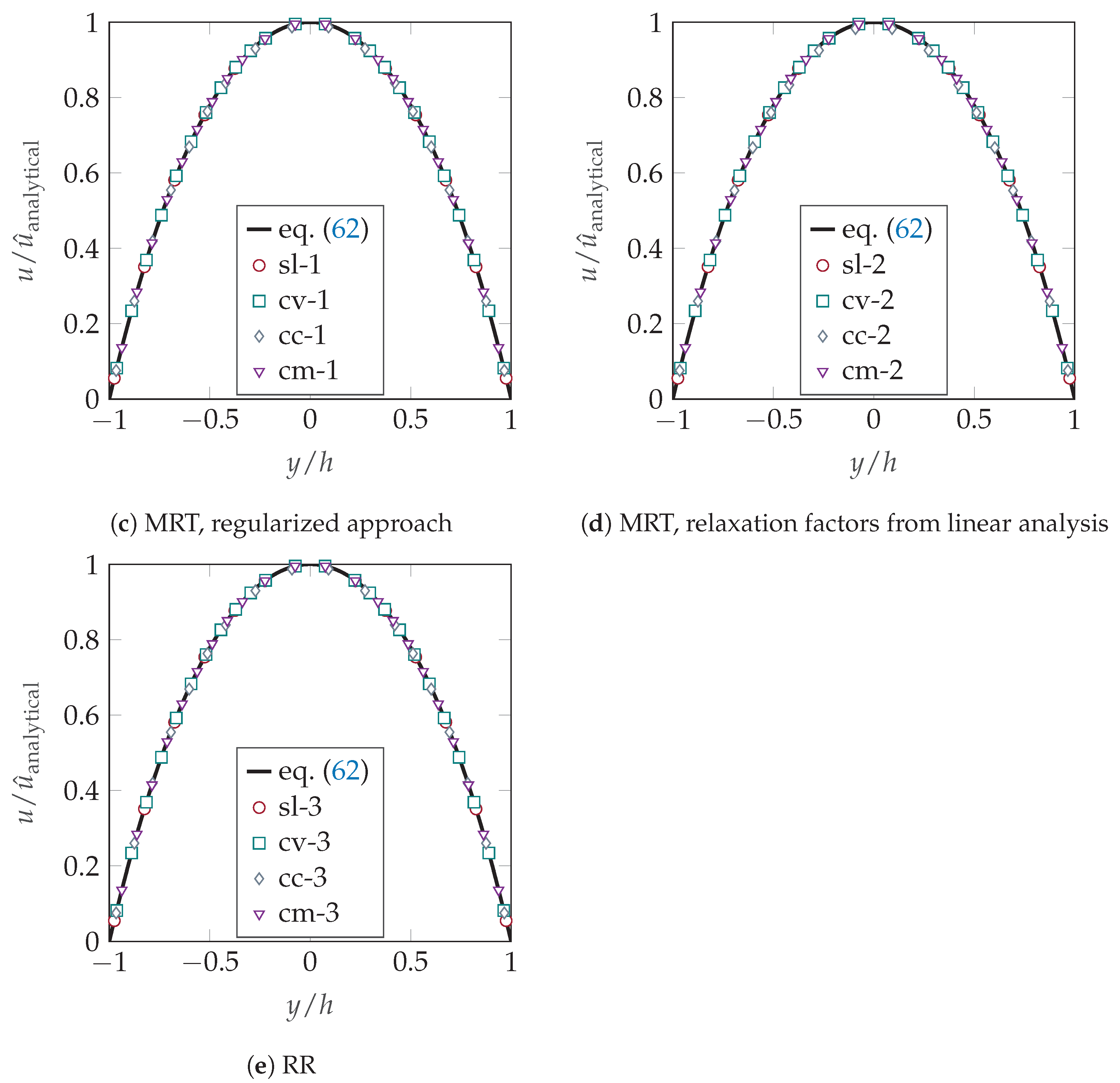
5.2. Verification
The conducted numerical experiments are verified by comparison with the analytical solution.
Figure 10 shows normalized velocity profiles (
in Equation (
62)) along
y direction normalized with half channel height
h, for all HRR cases with
and
, corresponding to a bulk Reynolds number of
. All simulation results agree very well with the solution in Equation (
62), supporting the correct numerical implementation of the adaptation of the HRR collision operator to the cell-centered and combined types of grid transition interface layout, as discussed in
Section 4. Velocity profiles for all other tested models exhibit similar agreement with the analytical solution and are shown in
Figure A2.
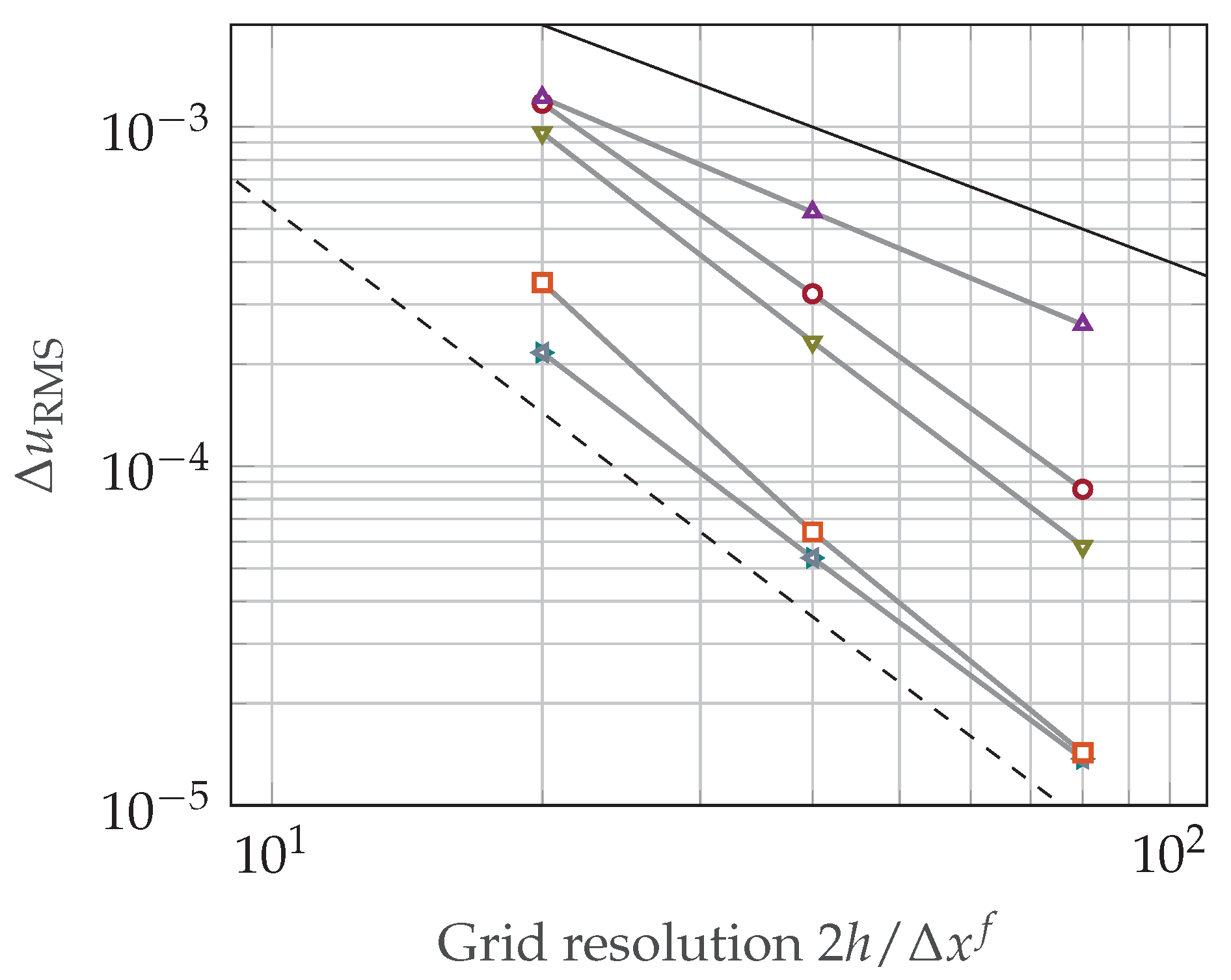
Numerical accuracy of the various grid transition schemes is further examined for the HRR collision operator by means of a grid convergence study, summarized in
Figure 11 in a double logarithmic manner. Results of the global absolute error in velocity averaged over all
N nodes, defined as
are given together with a slope of
and
for three successively refined grids, starting from the coarsest grid, which serves as the basis for stability experiments. Grid resolution is expressed in terms of number of respective fine level grid cells per duct height. The time step is determined by diffusive scaling
in order to ensure
convergence of the compressibility error, see
Table 3.
The validity and correctness of the presented HRR adaption for the cc and cm algorithms is again confirmed. The cc algorithm with linear explosion (
![Fluids 08 00103 i019]()
) shows an average slope of
, while the cm HRR adaption (
![Fluids 08 00103 i020]()
) results in an average convergence rate of
with a slight tendency of hyper convergence between the coarsest and medium grids, preserving the second order spatial accuracy of the LB scheme in a consistent manner. Relying on uniform particle redistribution during cc explosion (
![Fluids 08 00103 i021]()
), expectedly degrades the methods accuracy to first order with an average slope of
[
59]. Choosing a relatively low Mach number of
no difference between cv HRR including (
![Fluids 08 00103 i022]()
) and excluding (
![Fluids 08 00103 i023]()
) cubic correction terms
could be observed here, with both variants exhibiting an average slope of
. The single level method (
![Fluids 08 00103 i024]()
) yields an average convergence rate of
.
5.3. Accuracy and Stability Range Comparison
As mentioned, accuracy and stability range are considered in the context of the categories defined in
Section 5.1 for the test cases summarized in
Table 2. The decisive factor is the respective maximum value of
that just fulfills the conditions imposed on the category. Thus, for a concrete test case,
describes the maximum value of
with a precision of five significant digits, whereby the simulation satisfies the constraints
and
within a laminar flow regime. Similarly for
, the particular test case under consideration is at the stability limit, so it does not quite fall into the third category, since
does not occur.
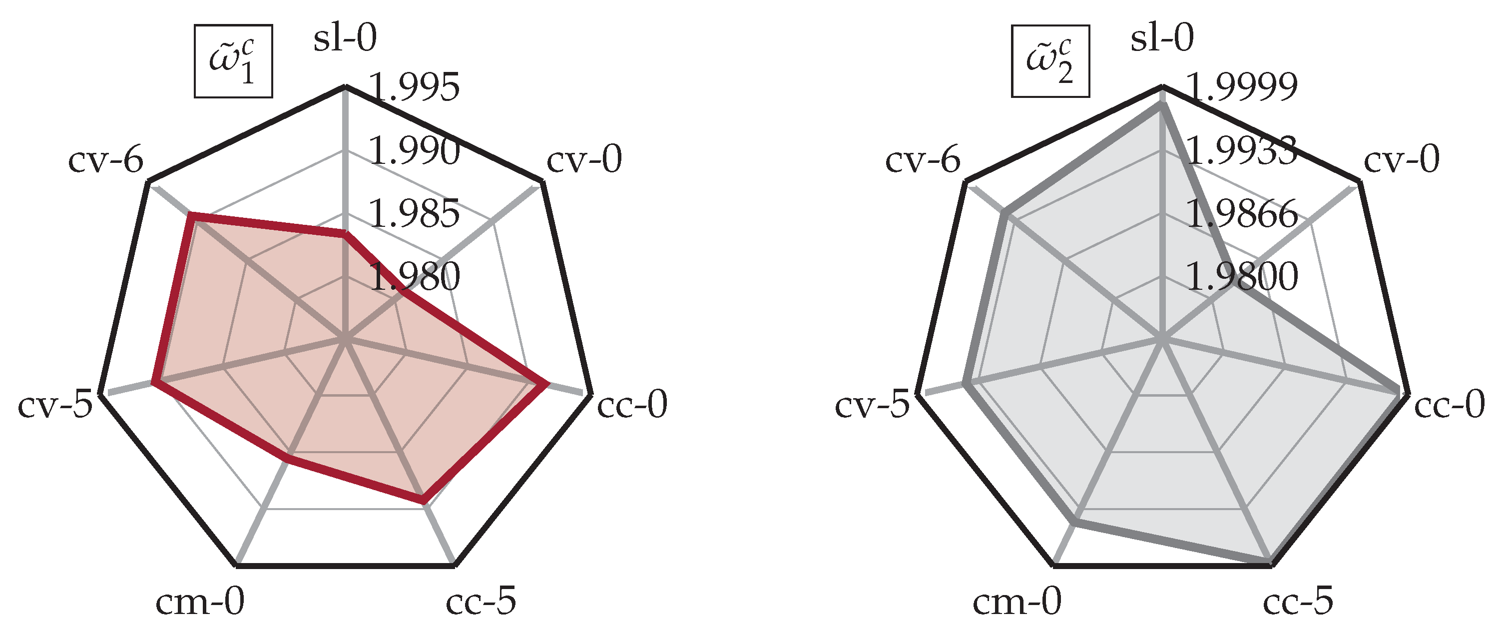
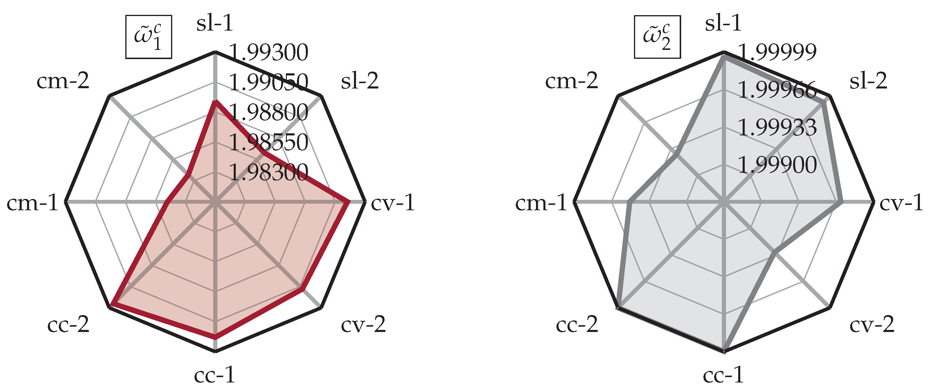
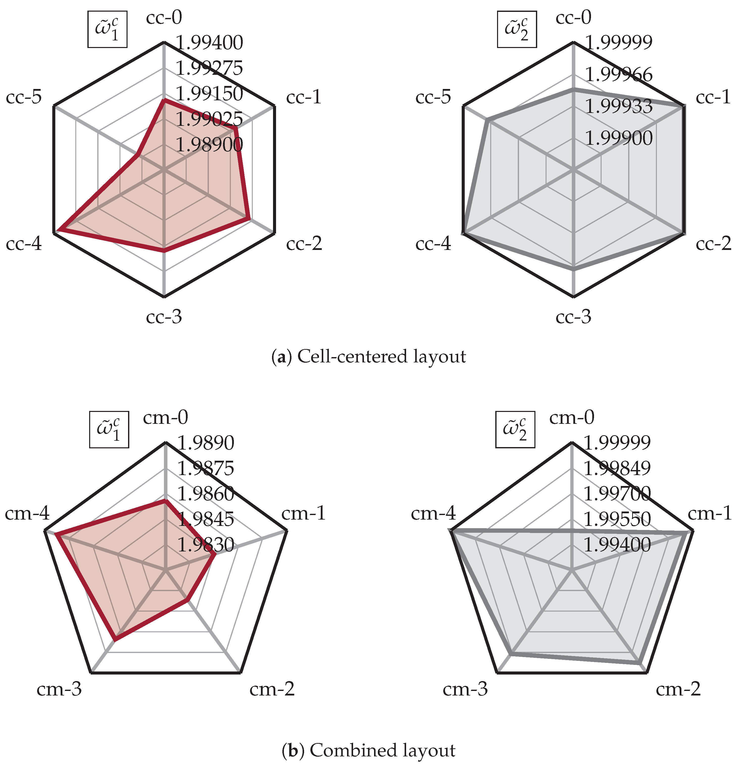
Figure 12 shows the maximum values
and
defined in this way for the BGK collision model for different grid layouts. It can be seen that the cell-vertex grid without additional restriction of the fine distributions denoted as cv-0 has the lowest values in both categories, with
(
) in category 1 and a clear distance to the other approaches in category 2 with
(
).
The cell-centered approach cc-5 with linear interpolation of the coarse post-collision distributions in the explosion step shows the highest stability of
(
) for the BGK collision model, closely followed by cc-0, i.e., uniform explosion, with
(
). Even though in the literature [
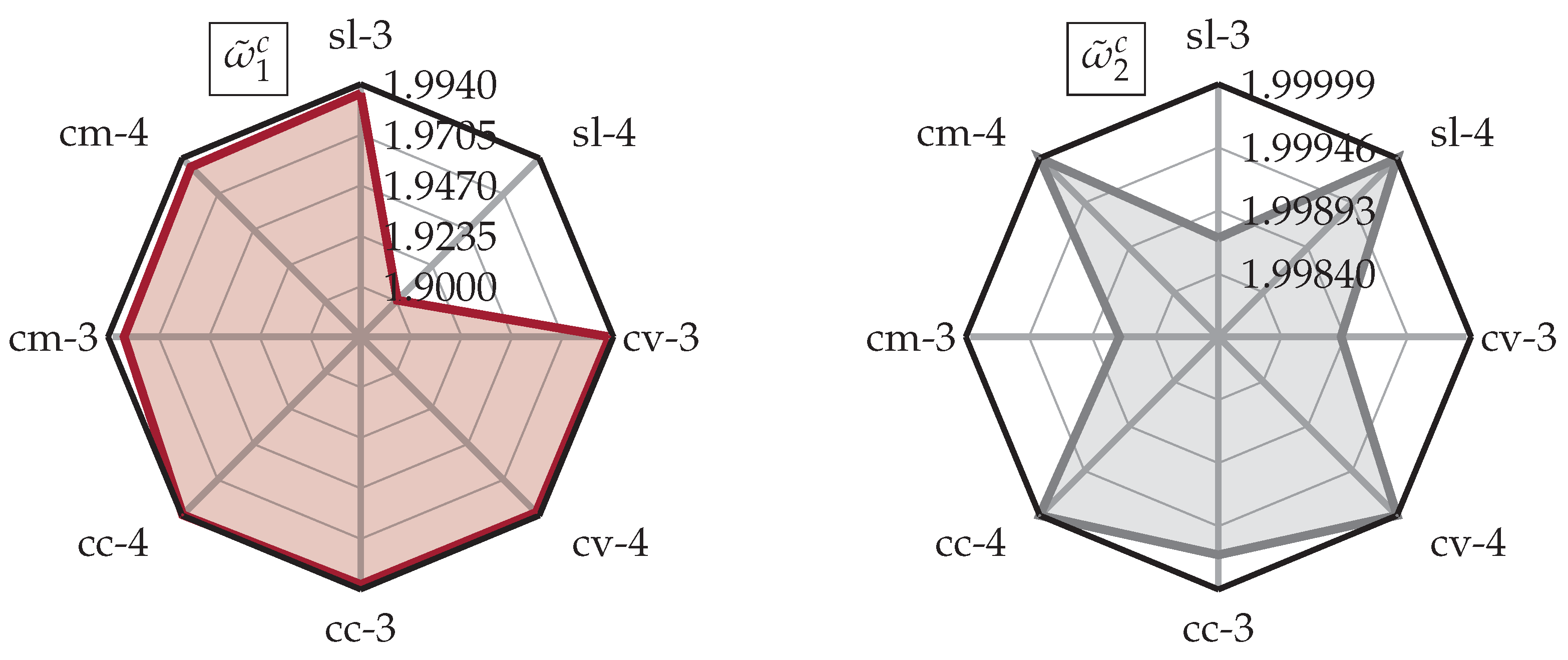
3,
56] physical justification for the
restriction step originally consisted in filtering out non-resolvable fine scales in turbulent flows, accuracy and stability range for the cv algorithm can be increased in our test case within laminar flow regime. Regarding category 1, the accuracy range can be expanded by including either filtering operation from Equations (
50) or (
51) into step 7 of Algorithm 1 to
(
) and
(
), respectively, exceeding the corresponding values of cc and cm. Stability range is increased to
(
) with both filters, which is in the immediate vicinity of
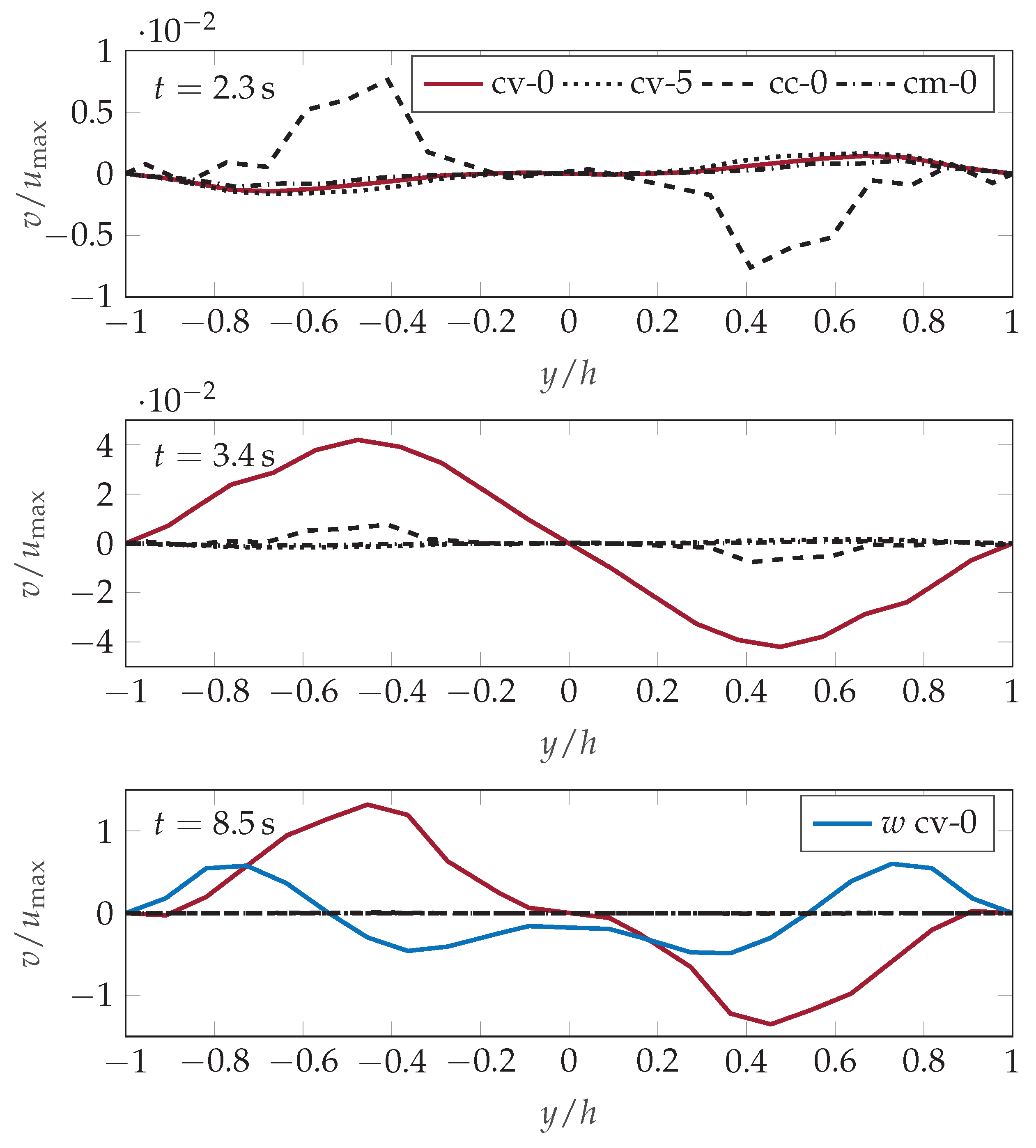
for the cm algorithm. The onset of instability is connected to the occurrence of spurious oscillations in the transverse velocity components
v and
w, the amplitude of which increases with time in the case of the cell-vertex algorithm without restriction (cv-0). This is shown in
Figure 13 along normalized
y direction for three exemplary chosen successive time steps and in comparison with the corresponding velocity values for cc-0, cm-0 and cv-5 (filtering according to Equation (
50)) at
(
), i.e., beyond cv-0’s stability limit. The spurious oscillation in transversal velocity
w is depicted only in time step
since its amplitude is several orders of magnitude below the
v-oscillation until that point and then increases rapidly.
When filtering is activated in the cv algorithm during the fine-to-coarse coupling step, as in cv-5, a significant suppression of these spurious oscillations comes into effect, yielding the simulation more stable. Due to the spatial separation of the fine and coarse interface nodes and the resulting implicit filtering of the distributions during the respective fine-to-coarse coupling (cf. Equations (
55) and (61)), this suppression of spurious oscillations occurs in equal form in the cc and cm layout. Differences in the curve characteristics at
between cv-5 and cm-0 on the one hand and cc-0 on the other, are possibly associated with missing scaling of
in the volumetric description.
As for the accuracy and stability range maps of the MRT collision model, both sets of relaxation parameters, the one obtained by von Neumann analysis and the one corresponding to a regularization step, are compared in
Figure 14. For all grid layouts except cc, MRT-REG (cases labeled -1) exhibits a slightly superior accuracy as well as stability range in the numerical experiments compared to MRT-NEU (cases labeled -2), while both MRT methods clearly surpass the BGK model in terms of stability. Even though MRT-NEU is explicitly calibrated to yield higher stability, regularizing the scheme by direct equilibriation of higher-order non-hydrodynamic moments as in MRT-REG seems to allow for further moderate stability gain. Between all grid transition types, the volumetric description again performs the strongest in terms of stability and also accuracy range with both MRT-REG and MRT-NEU exhibiting negative distribution functions at our terminal value
(
), followed this time by the cell-vertex algorithm. Differences to the cm algorithm are, however, of minor extent. Since stabilizing fine-to-coarse restriction is not active in our cv MRT test cases (cf. case overview in
Table 2), the stability increase with MRT-NEU and MRT-REG is probably associated to two aspects: An increase in bulk viscosity and non-hydrodynamic mode filtering, weakening any destructive and parasitic contributions that may occur, materializing in the form of spurious oscillations as seen with the BGK model. Any harmful artifact is thus attenuated before it can reach the grid transition interface to be amplified.
Figure 15 summarizes the values of
and
of the RR and HRR collision models for all grid layouts. Here again, differences between the cv algorithm on one side and cc and cm on the other in terms of stability range are overcome by the positive effects of the collision operator: The cell-centered algorithm leads in terms of accuracy range for both, the RR and HRR model and in terms of stability range for the RR model, followed again by the cell-vertex and combined layouts. It should be briefly mentioned here again, that the cc tests for all advanced collision operators except HRR have been contucted exclusively with uniform explosion (cf. Equation (
54)), that means with a degraded first order accuracy as can be seen in the grid convergence study for the HRR model in
Figure 11. Nonetheless, the differences in terms of stability range compared to linear explosion in Equation (
56) are negligable, as discussed above and depicted in
Figure 12 for BGK collision. Similarly, no difference has been observed in terms of stability range for HRR with linear explosion and only minor differences are present in the accuracy range map. For lucidity reasons, test case cc-6 is not depicted in
Figure 15 and an extension of the statements made here regarding cc’s stability range with uniform explosion can be attributed in a straightforward way to its linear enhancement.
The recursive-regularization step aims at filtering out non-hydrodynamic modes by explicit reconstruction of
according to Equation (
23). Although the basic idea is the same as in the MRT-REG model discussed earlier, differences in the stability ranges can be observed when both methods are compared to each other, more precisely, the RR model does exhibit slightly reduced stability. For example, cv MRT-REG remains in category 2 (cf.
Section 5.1) up to
(
), while cv RR remains stable only up to
(
), even though a third-order Hermite expansion of the equilibrium functions is used as compared to a second-order one in MRT model. An explanation for this can be found in the fact that the MRT model utilized here relies on a raw moment space built using the Gram–Schmidt orthogonalization procedure based on an unweighted scalar product [
30], while the populations in the RR framework are derived based on Gauss–Hermite quadrature. The specific choice of relaxation parameters in the MRT-REG model leads to an increased bulk viscosity compared to the RR model, contributing to the formers stability.
For the refined cases the highest values in terms of stability and accuracy range can be found for the Hybrid-Recursive Regularized collision model, regardless of the type of grid transition in use. All conducted HRR simulations remained in category 2 in our study, meaning no negative distribution functions have been detected up to the terminal value, thus yielding
(
) in all cases. Besides the non-hydrodynamic mode filtering properties of the HRR model [
12], its accompanying drastic stability increase is related to the injection of numerical hyper-viscosity through the usage of a hybridized computation of the stress tensor during the reconstruction of
, as expressed in Equation (
27) [
16,
31]. For the single level reference case however, the finite difference approximation of strain-rates within the stress tensor together with the rather coarse grid resolution leads to an early increase of the relative arithmetic mean error
beyond the
limit of category 1, as can be seen in
Figure 15 and
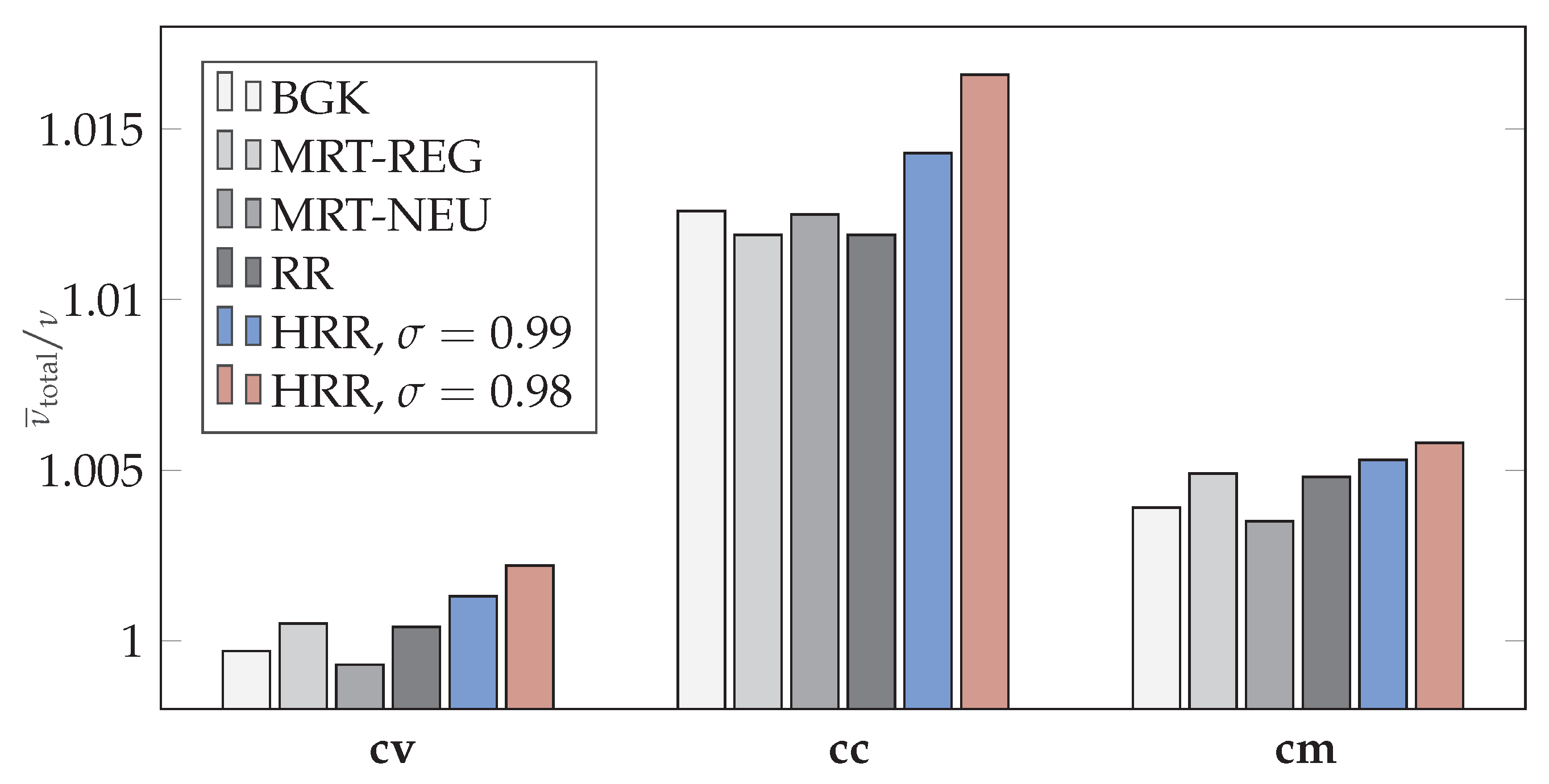
Figure 16a. The direct adjustment of the amount of numerical viscosity
through the hybridization factor
is depicted in
Figure 17 with
, corrsponding to a bulk Reynolds number of
. By inserting the numerical velocity into the analytical solution of the square duct flow (
62), solving for kinematic viscosity
and averaging over all nodes of the computational domain, the relative amount of total viscosity
is estimated for all collision models and grid transition algorithms. Interestingly, the RR and MRT-REG model lead to similar amounts of total viscosity for all grids, with the MRT-REG slightly above RR, besides showing differences in the stability ranges.
In addition to the values for the HRR hybridization factor used in the stability study, i.e.,
(corresponding to the RR model, cf. Equation (
27)) and
, the value of
is included. The linear trend of numerically induced hyper-viscosity can be clearly seen by comparing the RR (
) and two HRR cases with
and
, i.e.,
,
and
of stress tensor approximation through central finite differences, respectively. Whether the distinct stability gain with the HRR model could have been achieved with even higher values of hybridization factor, i.e., less added dissipation, will be left open for future work. Comparing the average levels of added numerical viscosity between individual grid transition schemes in
Figure 17 may give an explanation for the improved stability properties of the cc algorithm. The increased amount of dissipation introduced into the flow field relative to the other two approaches could be explained by the implicit filtering of the complete distribution function
during coalescence step 6 of Algorithm 3, as opposed to filtering only the non-equilibrium part
in step 7 of Algorithm 1 and step 5 of Algorithm 4. Lagrava et al. [
3] mentioned that they observed a strong dissipation by application of their averaging procedure in Equation (
50) to
or the macroscopic quantities
and
, which lead to the choice of filtering only
instead. Even though
is similarly interpolated trilinearly in our cm approach for the reconstruction of equilibrium functions
on interface nodes,
is obtained through a third-order polynomial expression. Moreover,
instead of
is interpolated trilinearly here. However, further research needs to be conducted on this regard.
While moderate differences between the grid transition algorithms are evident in terms of accuracy and stability range in
Figure 12,
Figure 13,
Figure 14 and
Figure 15 with the volumetric approach showing the highest values for
, the influence of the collision operator is considerably greater in this respect. This is made even more apparent by a rearrangement of the range maps juxtaposing different collision operators for each individual grid transition algorithm as it is shown in
Figure 16 and
Figure 18. Regardless of the specific interface type in use, the highest values of
is achieved exclusively with the HRR collision model, extending beyond the scope of
(
) of our numerical experiments, closely followed by the two MRT models and then RR, with MRT-REG slightly above MRT-NEU and lastly BGK.


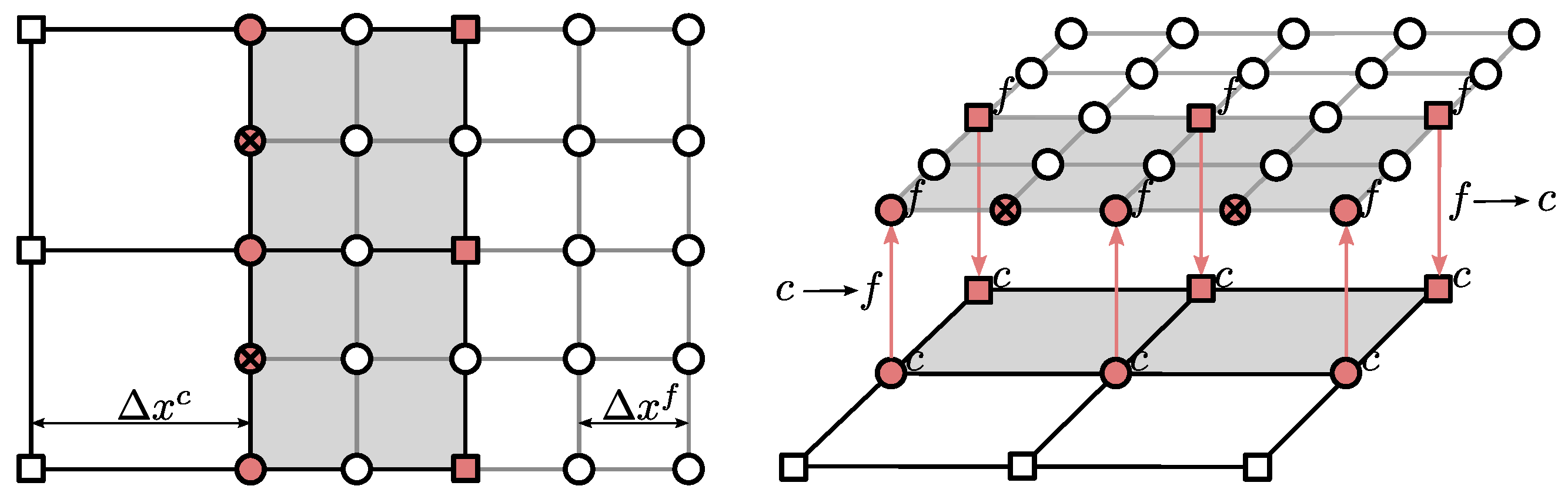
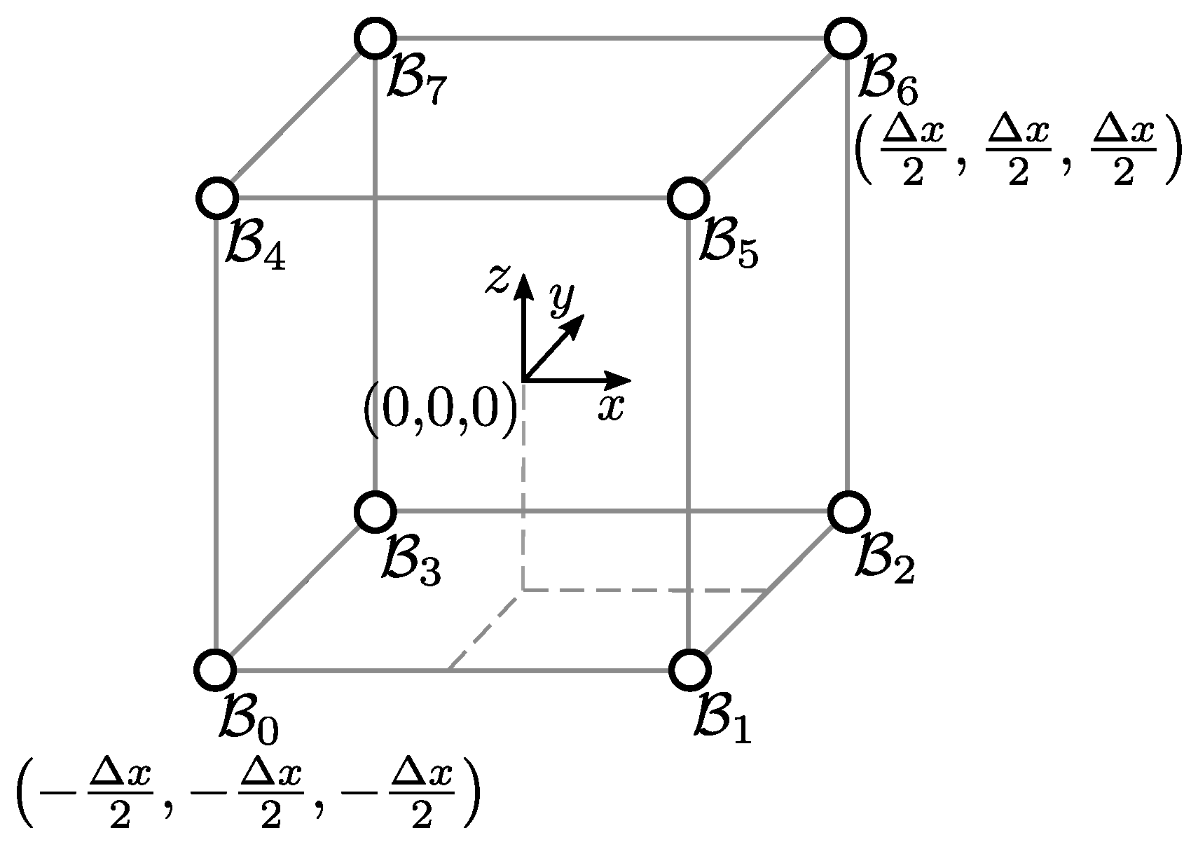
 and the fine grid
  , hanging middle nodes
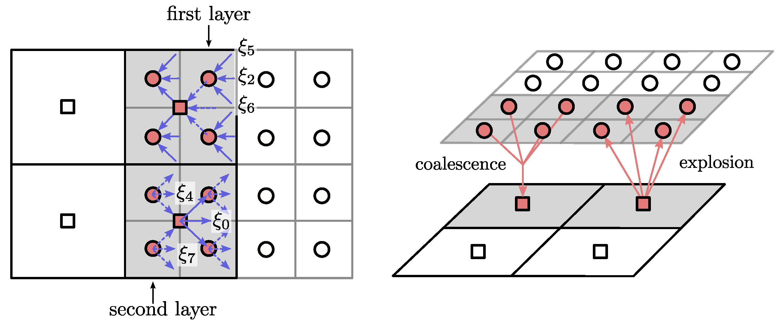
  lacking neighbors on the same level in at least one direction and are therefore missing the corresponding populations after streaming. The missing information is recovered using co-located grid nodes, referred to as partner nodes
  and
and  , belonging to the other grid, under the condition that a smooth transition of hydrodynamic quantities such as density , fluid momentum and the viscous stress tensor is ensured across the interface.
 , if they reside in a cell face center, as depicted in Figure 4 for three spatial dimensions. Missing populations at these nodes are determined through cubic [51] and bi-cubic [52] polynomial interpolation, respectively, using information of neighboring fine nodes with coarse partners. With stencil numeration as illustrated on the right side of Figure 4, interpolation formulas for middle and center nodes become


 , which are also utilized in the central difference stencil and temporally evolve directly from t to . After the fictitious streaming step, a valid velocity vector can be extracted from the updated fine partners.

 , are redistributed among fine interface nodes
  contained within the same coarse parent cell. This procedure will be referred to as uniform explosion, since particle mass is homogeneously distributed, without any type of spatial or temporal interpolation applied. Since two rows of fine interface nodes are supplied with coarse post-collision states, they remain valid for two consecutive fine time steps. Furthermore, according to [5] no rescaling of non-equilibrium distributions is performed, in contrast to the cell-vertex method in Algorithm 1. To keep the algorithmic description consistent between grid layouts, mathematical notation of grid coupling steps in the cell-centered scheme will be expressed in terms of particle densities, rather than masses. Explosion then implies equality between particle densities, and coarse provider and fine receivers. With post-collision distribution functions symbolized by , the explosion step is simply given as:
 will be referred to as first-layer nodes, whereas second-layer nodes means fine interface node devoid of regular fine neighbors. Particle collision does not take place at first- or second-layer nodes, so that collision has to be performed at the coarse receiver node after coupling. In terms of particle densities, this as coalescence known procedure implies missing coarse densities to be obtained by averaging fine particle densities contained within the coarse cell, resulting in the following expression for D spatial dimensions:
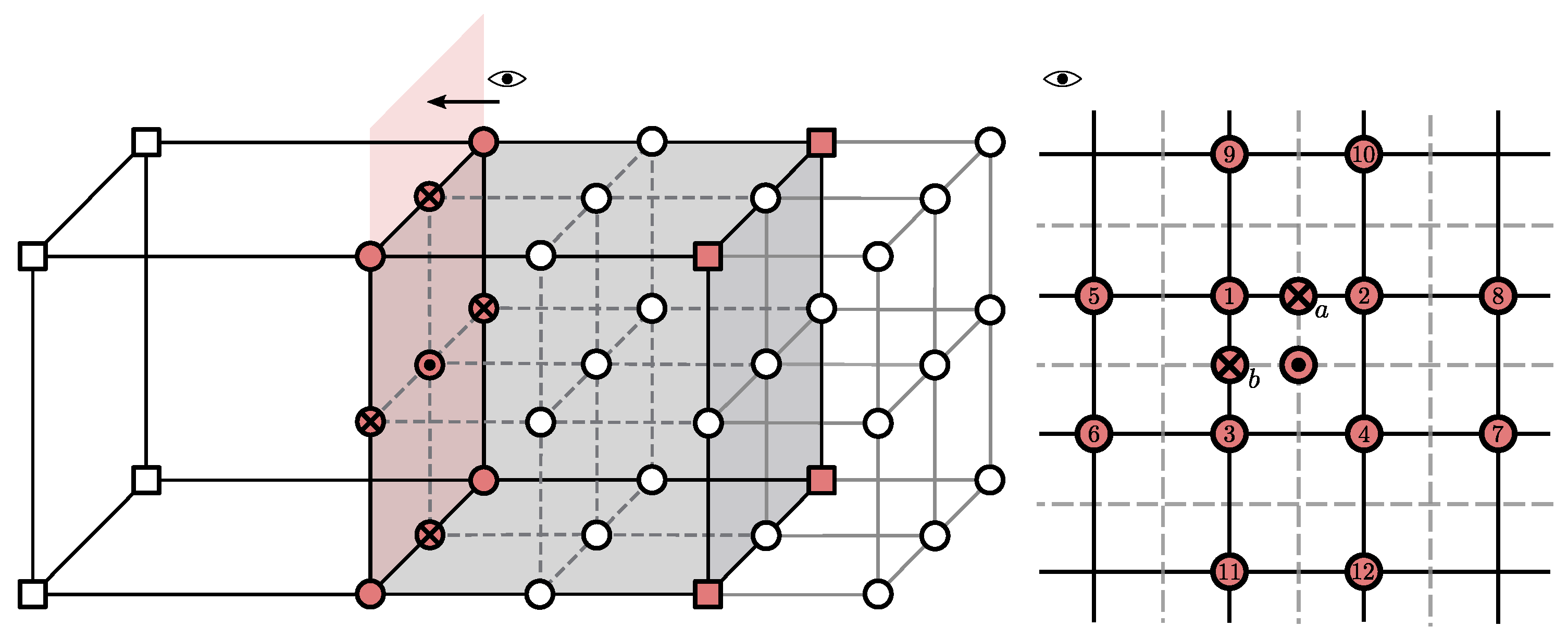
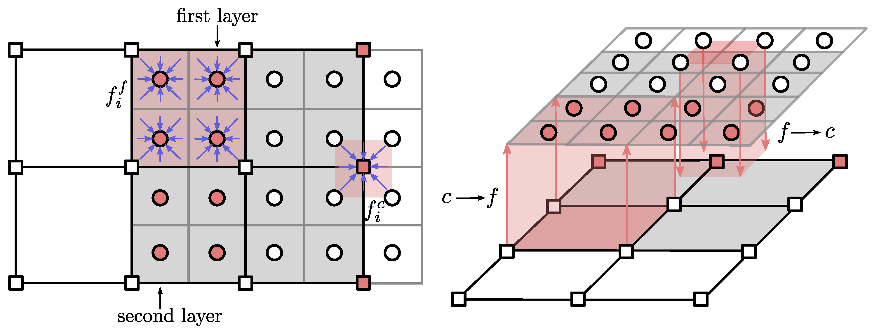
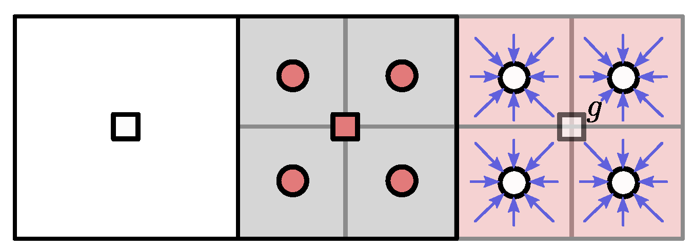
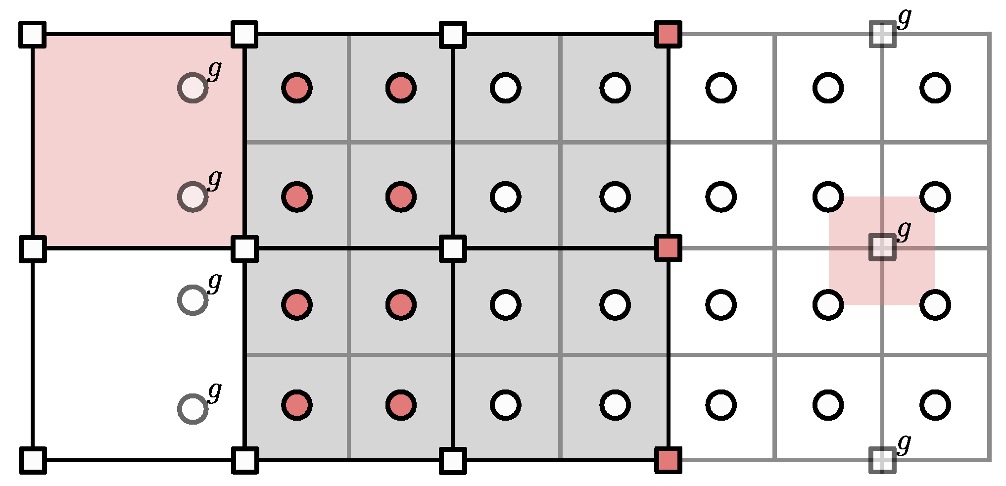
 , using a fictitious coalescence at regular fine nodes covering its image. Fine pre-collision distribution functions in all directions are averaged according to Equation (55) and thus provided for a calculation of the macroscopic velocity within the strain-rate computation at
  ghost nodes in Figure 8, to achieve a central finite difference stencil relative to second-layer and coarse interface nodes. This modification is included into step 1 of the combined Algorithm 4.
 ) shows an average slope of , while the cm HRR adaption (
 ) results in an average convergence rate of with a slight tendency of hyper convergence between the coarsest and medium grids, preserving the second order spatial accuracy of the LB scheme in a consistent manner. Relying on uniform particle redistribution during cc explosion (
 ), expectedly degrades the methods accuracy to first order with an average slope of [59]. Choosing a relatively low Mach number of no difference between cv HRR including (
 ) and excluding (
 ) cubic correction terms could be observed here, with both variants exhibiting an average slope of . The single level method (
 ) yields an average convergence rate of .


