Classification of Cocoa Pod Maturity Using Similarity Tools on an Image Database: Comparison of Feature Extractors and Color Spaces

Abstract

Côte d’Ivoire, the world’s largest cocoa producer, faces the challenge of quality production. Immature or overripe pods cannot produce quality cocoa beans, resulting in losses and an unprofitable harvest. To help farmer cooperatives determine the maturity of cocoa pods in time, our study evaluates the use of automation tools based on similarity measures. Although standard techniques, such as visual inspection and weighing, are commonly used to identify the maturity of cocoa pods, the use of automation tools based on similarity measures can improve the efficiency and accuracy of this process. We set up a database of cocoa pod images and used two feature extractors: one based on convolutional neural networks (CNN), in particular, MobileNet, and the other based on texture analysis using a gray-level co-occurrence matrix (GLCM). We evaluated the impact of different color spaces and feature extraction methods on our database. We used mathematical similarity measurement tools, such as the Euclidean distance, correlation distance, and chi-square distance, to classify cocoa pod images. Our experiments showed that the chi-square distance measurement offered the best accuracy, with a score of 99.61%, when we used GLCM as a feature extractor and the Lab color space. Using automation tools based on similarity measures can improve the efficiency and accuracy of cocoa pod maturity determination. The results of our experiments prove that the chi-square distance is the most appropriate measure of similarity for this task.

Dataset: https://doi.org/10.17632/9msjjh3np6.2.

Dataset License: CC BY 4.0

1. Introduction

Côte d’Ivoire is a country located in West Africa known to be the world’s largest cocoa producer [1,2]. Cocoa is an essential crop for the country’s economy and is grown in several regions, providing livelihoods for thousands of people. However, the quality of the cocoa strongly depends on the maturity of the cocoa pods, which must be taken into account during harvesting. The quality of the cocoa has a direct impact on the selling price. When cocoa is of high quality, it is usually sold at a higher price, which will allow farmers to produce higher quality cocoa to generate more significant income [3]. By improving the quality of cocoa through automated methods of detecting the maturity of cocoa pods, farmers could obtain higher incomes for their work. Improving the quality of cocoa will also positively affect the environment and the sustainability of the cocoa industry [4]. This is because immature cocoa pods do not contain as many cocoa beans as mature pods, which implies that more pods must be harvested to obtain the desired quantities of beans. This will lead to overexploitation of natural resources and agricultural land, as well as higher costs for farmers in terms of labor and energy. By improving the detection of the maturity of cocoa pods, it may be possible to reduce the quantity of pods harvested and thus reduce the environmental impact of the cocoa industry. It is important to remember that Côte d’Ivoire is the largest cocoa producer in the world, with an annual production of more than 2 million tons of cocoa beans, and any system allowing the improvement of the quality of cocoa will significantly impact the cocoa industry worldwide [5]. In this context, detecting the maturity of cocoa pods is crucial for improving the quality of the final product [6]. Most of the time, this detection is carried out manually, and it requires a lot of time and carries a risk of error in the interpretation. Technological advances may allow the development of automated methods to detect the maturity of cocoa pods, particularly by using cocoa pod images [7]. Using automated methods to classify cocoa pods according to their maturity would improve the quality of the final product and optimize yields. This would have positive impacts on farmers’ incomes and the country’s economic growth.

Classification methods are widely used in various applications to group similar data. One of the critical elements of data classification is the measure of similarity, which makes it possible to determine the proximity between different observations or examples. Classification methods based on similarity measures focus on comparing the features of each item to assess their similarity or difference [8]. They are, therefore, essential for classification methods and many applications, such as market analysis, pattern recognition, and image classification.

The traditional method of detecting the maturity of cocoa pods relies on the expertise of the selectors, which can be subjective and vary from picker to picker. Using an automated method to classify images would allow a more objective and precise evaluation of the maturity of cocoa pods.

This article uses image processing techniques to discuss the maturity classification of cocoa pods from an image database. This study aims to compare different feature extractors and color spaces to determine the most efficient method to classify the maturity of cocoa pods from images.

Our study made the following contributions:

• We created a dataset named CocoaMFDB [9], which contains RGB images of cocoa pods taken under varying light conditions. To improve the quality of these images, we applied the contrast-limited adaptive histogram equalization (CLAHE) algorithm and extracted cocoa pods from each image. We applied a data augmentation technique for each pod based on Deep Learning. This dataset is open and can be used for various purposes.
• We took our RGB datasets and transformed them into several color spaces, such as HSV, Luv, and Lab. Then, we extracted features from each image for each color space using GLCM and CNN feature extractors.
• We used mathematical similarity measurement tools, such as the Euclidean distance, correlation distance, and chi-square distance, to classify the extracted features in each color space.
• In the present manuscript, we compared the experimental results for each combination of feature extractor and color space according to our research methodology. The results of these comparisons were included in our analysis and are presented in the appropriate section of this document.

2. Related Work

Several studies have been conducted in this direction; Liao et al. proposed a method of segmentation of rice plants based on the colorimetric space, which consists of the graying of the image. The image is converted from RGB color space to YCrCb color space. A 2Cg-Cb-Cr color index is then constructed to gray out the image on the excess green index, which reduces the influence of lighting variation. This method allowed us to obtain better segmentation results and reduced the computational cost compared to the process [10]. Wen et al. proposed an approach based on the YUV color space with the YUV-GAN method that eliminates end-to-end thin clouds by independently learning the luminance and chrominance components, which is effective in reducing the number of bright and dark pixels that are unrecoverable [11]. Jawahar et al. have, in their study, used a method based on the colorimetric space based on Lab for the segmentation of the diabetic foot ulcer [12]; Cao et al. based their study on two classic methods of automatic colorization, the Welsh approach and the Gupta approach, and the experimental results demonstrate that YCrCb and YIQ have better performance in texture similarity than Lab and LUV for both methods of color transfer [13]. Chagas et al. evaluated in their study CNN models for image classification, and these models outperformed conventional methods [14]. Behera et al. proposes a method for the classification of papaya fruit maturity, using VGG-19 with a transfer learning approach, which achieves better accuracy than the existing method [15]. Espejo-Garcia et al. implemented a solution based on feature extraction from deep layers of multiple transfers learning CNN models for automatic crop and weed detection [16]. Bueno et al. studied a technique to determine the degree of maturity of cocoa based on the acoustic sound of cocoa pods. Their approach enabled extracting recognizable features for the training process and then applying the convolutional neural network to classify cocoa bran. The experimental model gave 97.46% accuracy of the classification system on the question of maturity of unripe and ripe pods [17]. De Oliveira et al. used an approach that involved studying a deep network-based classification model built on the Inception-Resnetv2 model to identify cocoa pods in their environment to differentiate ripe cocoa pods before harvest. The results obtained at the end of their study gave an accuracy of 90% [18]. The use of combined parameters, such as color, pH, and acidity, have been used by Cubillos Bojacá et al. to identify the degree of ripeness of cocoa fruits. This approach gives indicators of maturity to planters for a better raw material in the chocolate industry [19]. Ma et al. developed a novel strategy to construct sequential features from a single image in short-term memory (LSTM) with the use of two pixel-based similarity measures, including pixel matching (PM) and l block matching (BM), used for the selection of sequence candidates from the entire image. Then, the sequence structure of a given pixel can be constructed as an input of LSTM using the first matching pixels with high similarities [20].

3. Materials and Methods

The experiments were conducted using Python programming on a DELL desktop computer in the ImVIA laboratory. The computer has an Intel(R) Core i7-10700 CPU at 2.90 GHz, 32 GB of RAM, and an NVIDIA Quadro P400 GPU. Models are configured in Python version 3.8.8 using Keras API version 2.4.3 with Tensorflow version 2.3 backend and CUDA/CuDNN dependencies for GPU acceleration.

3.1. Data Description

3.1.1. Data Acquisition

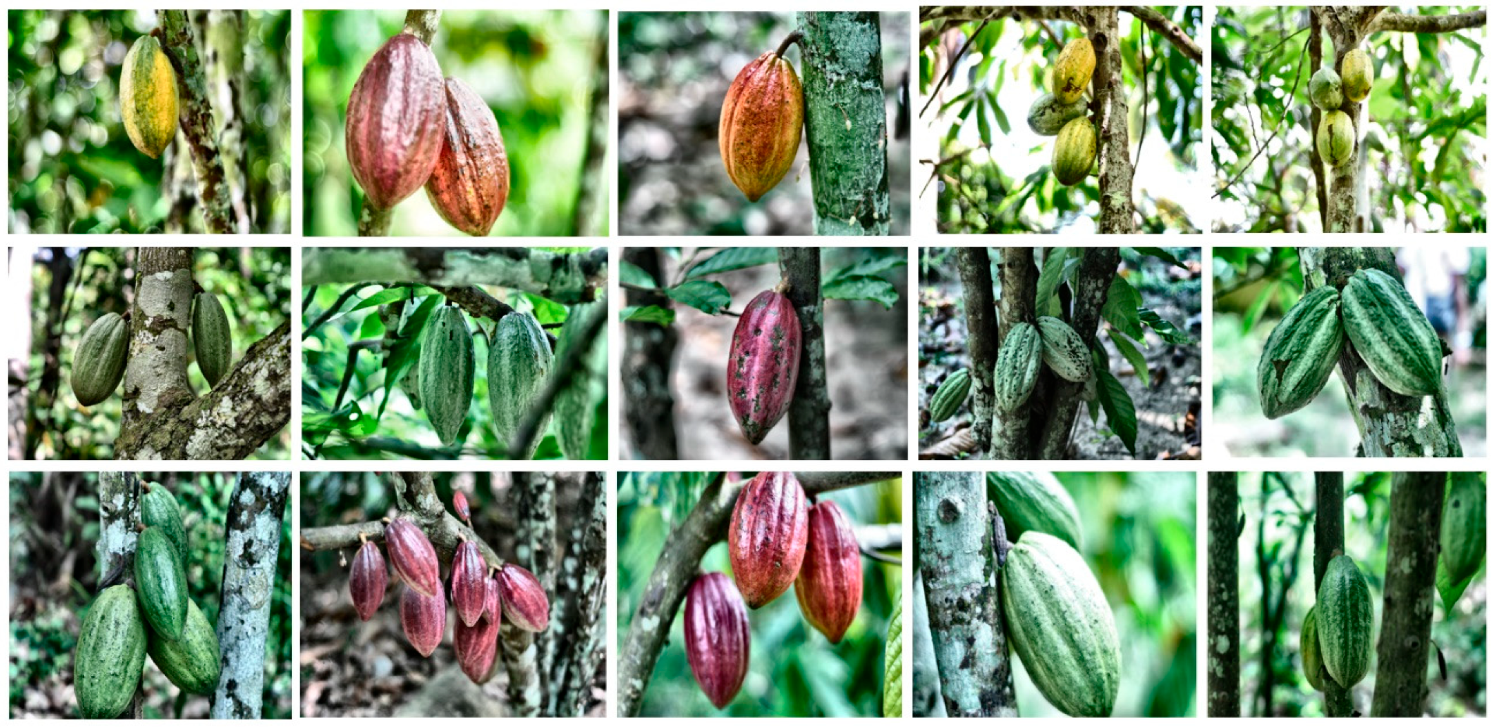
The dataset we use is called CocoaMFDB [9]. It comprises 1254 images of cocoa pods in different states of maturity, namely, mature and unmatured. Each image contains multiple pods. The images were taken using Nikon D500 is a DSLR camera manufactured by Nikon, a Japanese company specializing in imaging and optical products. Nikon’s headquarters are located in Tokyo, Japan and Infinix cameras at a cocoa plantation at Yakassé 1 in Ivory Coast. The pods were photographed in an uncontrolled environment from several angles and at different times of the day to approximate the observation of the planter. Figure 1 shows an example image of our dataset.

3.1.2. Data Preprocessing

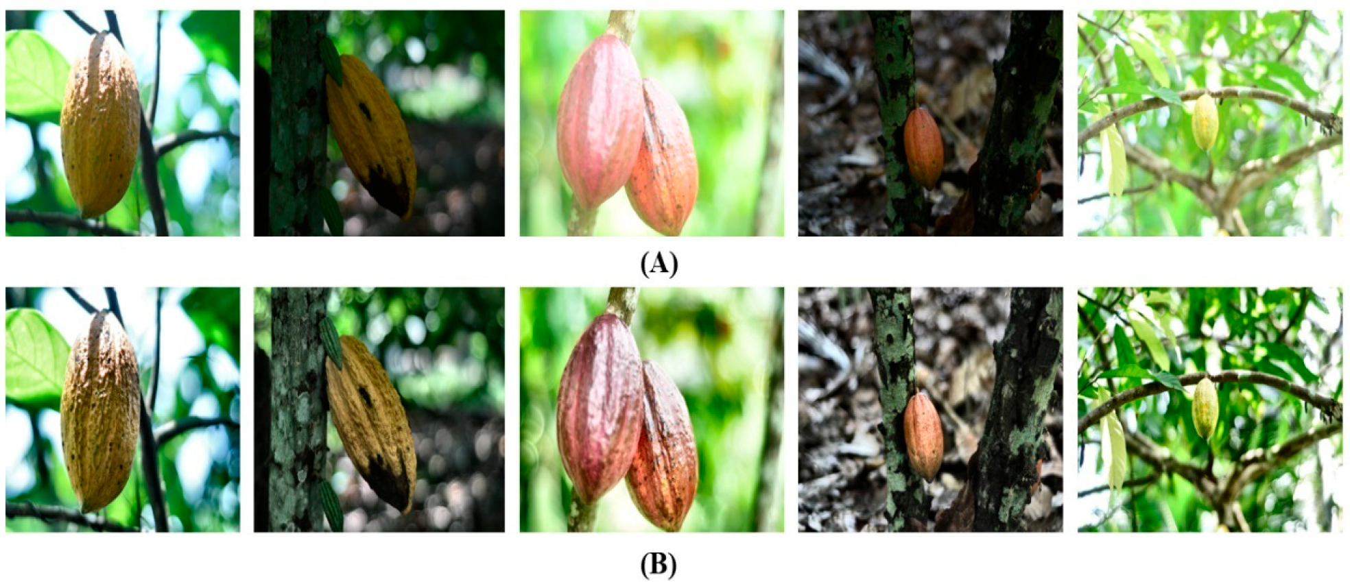
Data preprocessing is a crucial step in any data processing process, as it cleans and optimizes data before using them in a model or application. In the case of image analysis, preprocessing is particularly important because images can contain a lot of noise and variations that can negatively affect image quality [21]. Image preprocessing usually involves several steps, such as normalization, segmentation, filtering, histogram equalization, etc. Histogram equalization is a commonly used image processing technique to improve image quality. The CLAHE (Contrast Limited Adaptive Histogram Equalization) algorithm is a popular histogram equalization method suitable for images with contrasting local variations [22]. The CLAHE algorithm was used in the preprocessing. CLAHE works by dividing the image into small regions called tiles and applying histogram equalization to each tile individually. This makes it possible to adapt the histogram equalization to each part of the image rather than applying a global equalization to the whole image. Next, neighboring tiles are combined using bilinear interpolation to avoid artificial borders that might appear between tiles.

Subsequently, a Gaussian filter is applied to attenuate local variations in the image and to smooth the image to improve the overall visual quality of the image. The Gaussian filter is a type of linear filter that attenuates the high frequencies of the image while preserving the low frequencies [23]. It can be used to reduce image noise, smooth image edges, and improve overall image quality. Figure 2 shows the effect of preprocessing on our images after acquisitions.

3.1.3. Data Creation

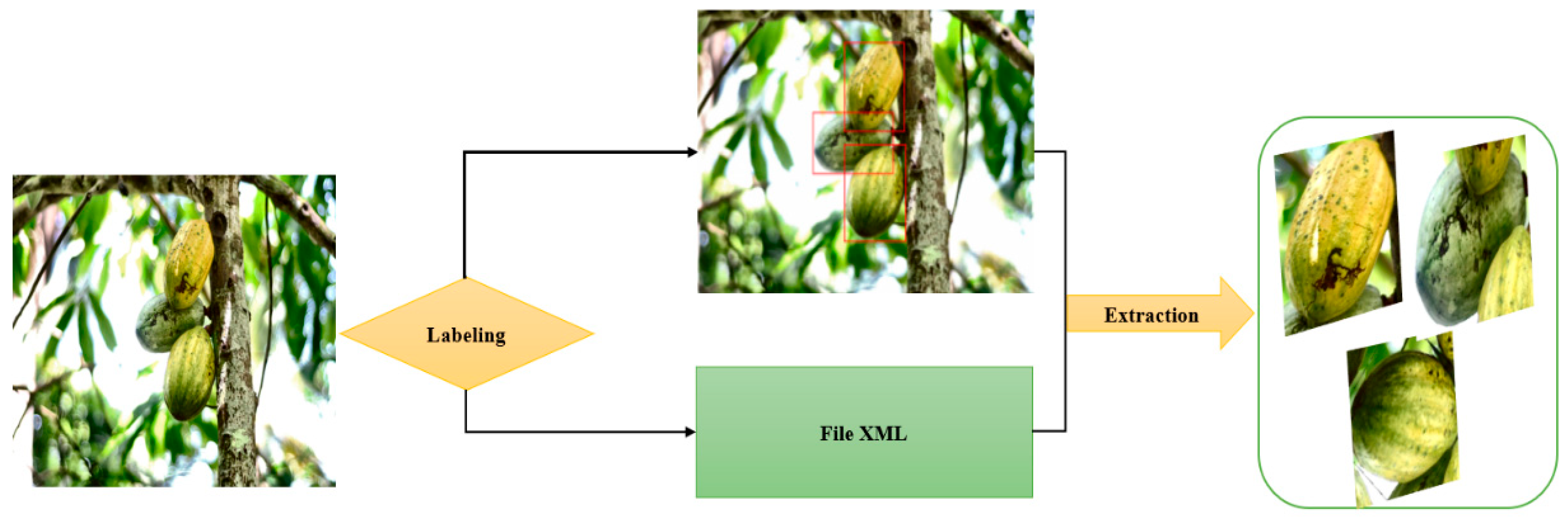
Thanks to the Labeling [24] annotation tool, we managed to identify and label the cocoa pods present in the images of our dataset. This image annotation method allowed us to create a labeled dataset, which will be used to perform cocoa pod detection or classification operations. Labeling the cocoa pods on the images allowed us to build a quality dataset that was used in object feature extraction methods. The original images were saved in JPG format, and the XML file containing the pod information was created. The process of extracting pods from images is shown in Figure 3.

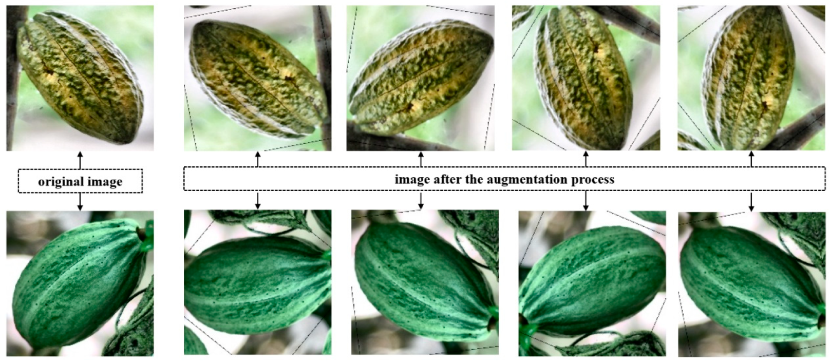
When making robust classifications of a dataset, it is essential to have enough data to guarantee a balance between the different classes of data. To achieve this, we increased the number of data samples by performing data augmentation. Data augmentation is a common technique to improve the performance of machine learning models by allowing the model to see a greater variety of images during training [25]. This can help avoid overfitting and improve model performance on new data.

The data augmentation process has two main operations involved in the image transformation operation, which is randomly applied to each input image. These operations are as follows:

• The first transformation is a horizontal and vertical random translation of pixels in the image.
• The second transformation is a random rotation of the image clockwise or counterclockwise with a maximum rotation angle of 0.4 radians.

By combining these two image transformation operations, this function helps generate new images from the original dataset to increase the dataset’s size and improve the model’s performance by generalizing better on the test data.

This method resulted in a balanced dataset, with a total of 9309 pod images, including 4660 ripe pod images and 4649 unripe pod images. Figure 4 clearly illustrates the increase in the number of pod images after data extraction, which improved the quality of our classification methods.

3.2. Color Space

Color space is a representation system that describes colors using mathematical coordinates. Colors are often described in terms of their hue, saturation, and lightness [26]. Different color spaces have been developed to meet the needs of other application areas, such as photography, printing, video, and graphic design.

• RGB (red, green, blue) color space: an additive system in which colors are created by mixing different amounts of red, green, and blue light [27]. The values for each channel range from 0 to 255, giving a total of over 16 million possible colors. The RGB model is primarily used for color representation on computer monitors and televisions, and digital images are often stored as arrays of RGB pixels [28].
• HSV (hue, saturation, value) color space: a system that describes colors in terms of their hue, saturation, and lightness [29]. Hue is represented by an angle from 0 to 360 degrees, a value represents saturation from 0 to 100%, and a value represents a value from 0 to 100%. Hue describes the color itself, saturation describes the amount of gray mixed with the color, and value describes the lightness of the color. The HSV model is often used for image processing, design color, and color selection [30].
• Lab color space: a color system that describes colors in terms of their lightness (L), a-chromatism (a), and b-chromatism (b). The brightness varies from 0 to 100, and the a and b values are centered around zero. The Lab color space describes all colors visible to the human eye, including colors that cannot be represented in other color spaces [31]. It is often used for color correction and comparison in graphics, printing, and photography applications.
• Luv color space: a color system similar to Lab color space, but it uses a different method to describe the color’s chrominance (U and V) [32]. The Luv color space uses a non-linear transformation to improve the accuracy of chroma description. Like the Lab color space, the Luv color space is used in graphics, printing, and photography applications for color correction and comparison [33].

Each color space has advantages and disadvantages depending on the application for which it is used. The RGB model is often used for color representation on computer monitors and televisions, while the HSV model is often used for image processing, design color, and color selection. LAB color space and LUV color space are used in graphics, printing, and photography applications for correction.

3.3. Feature Extractors

Feature extractors are algorithms that transform raw data into a relevant and easily usable representation to perform operations, such as classification, machine learning, etc. They are used in many fields, such as computer vision, natural language processing, speech recognition, biology, and chemistry [34].

The goal of feature extractors is to reduce the dimensionality of the data, i.e., to go from a large number of features to a much smaller number. They make it possible to simplify the data, to make them less complex during classification operations, and, thus, to reduce the calculation times necessary to carry out the classification or learning operations.

There are several types of image feature extractors [35], including:

• Color-based feature extractors: these extractors use color as the main feature to describe an image.
• Texture-based feature extractors: these extractors use texture patterns in an image to extract features.
• Edge-based feature extractors: these extractors use the edges and edges of the image to extract features.
• Convolutional neural networks (CNN): these extractors use deep neural networks to extract features from an image. CNNs have succeeded in many image-processing applications, including image classification and object detection [36].
• Shape descriptors: these feature extractors are designed to extract features based on the shape of objects in an image.
• Fourier Transform: This technique transforms an image into a series of frequencies to extract features, such as horizontal and vertical lines.

We used two feature extractors in this study: the GLCM, which is a texture-based extractor, as well as the MobileNet, which is a convolutional neural networks-based extractor.

3.3.1. Gray Level Co-Occurrence Matrix (GLCM)

The GLCM (Gray Level Co-occurrence Matrix) feature extractor is a texture-based image analysis technique [37]. It measures the relationship between the gray levels of pixels in an image by considering the spatial proximity of these gray levels. This technique thus makes it possible to extract essential features from images, which can then be used in classification, segmentation, object recognition, etc.

The GLCM computes a gray-level co-occurrence matrix for each pixel in the image, considering some directions and distances [38]. The matrix thus obtained is then normalized and can be used to extract different characteristics, such as energy, homogeneity, entropy, correlation, etc. The equation of the other elements is:

$$Contrast={\displaystyle \sum }_{i,j=1}^N{P}_{i,j}{\left(i-j\right)}^2$$

(1)

$$Dissimilarity={\displaystyle \sum }_{i,j=1}^N{P}_{i,j}\left|i-j\right|$$

(2)

$$Homogeneity={\displaystyle \sum }_{i,j=1}^N\frac{P_{i,j}}{(1+{\left(i+j\right)}^2)}$$

(3)

$$Energy= \sqrt{{\displaystyle \sum }_{i,j=1}^N{P}_{i,j}^2}$$

(4)

$$Correlation={\displaystyle \sum }_{i,j=1}^N{P}_{i,j}\left[\frac{\left(i-{\mu }_i\right)\left(j-{\mu }_j\right)}{\sqrt{({\sigma }_i^2)({\sigma }_j^2)}}\right]$$

(5)

With i, j represents the spatial coordinates of the function P(i,j), N is the gray level, σ represents the variance of GLCM, and the variance μ represents the mean.

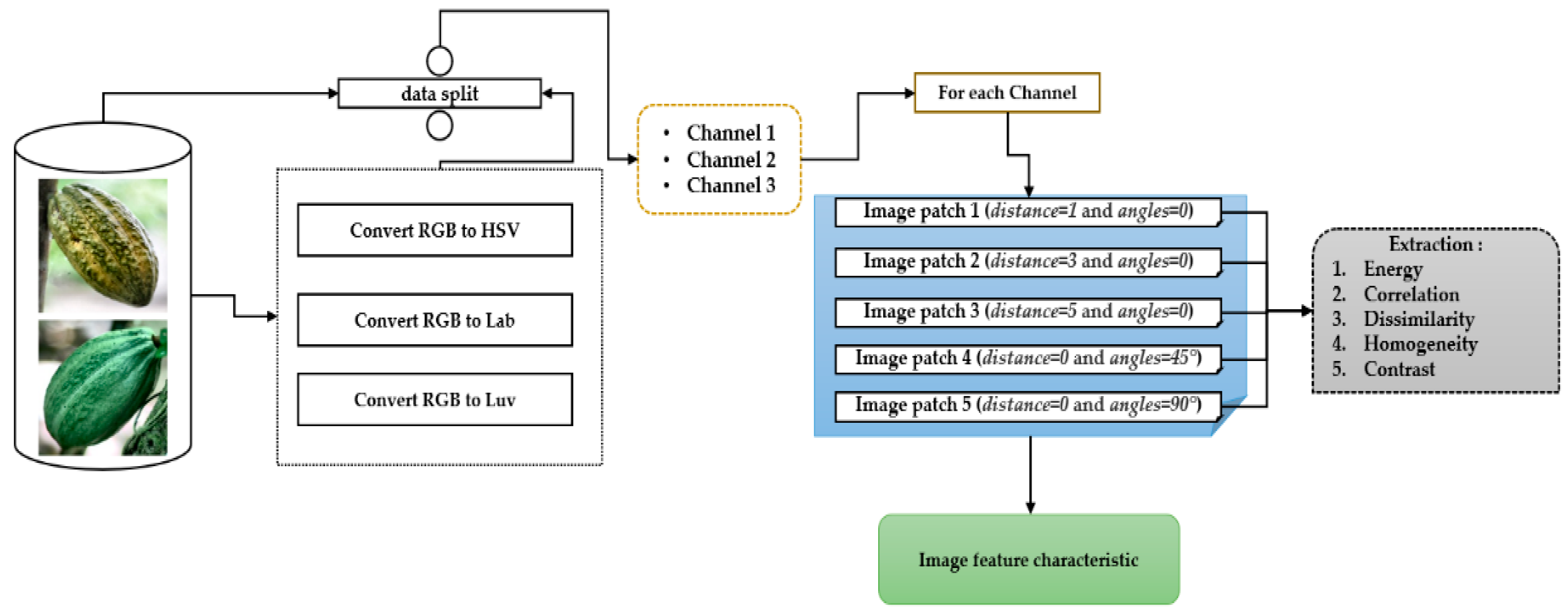
In our study, for each image, we extract the feature of each image channel using different patches of the image with the extraction of the parameters mentioned above. Figure 5 shows the extraction based on the GLCM.

Figure 5 describes the following function:

The purpose of the function is to extract features from a series of images in our database.

• Step 1: For each image in our database, the function creates a temporary data frame that will be used to store the features extracted from the image being processed.
• Step 2: The function calculates several properties of the grayscale co-occurrence matrix (GLCM) for each color channel in the image.
• Step 3: For each color channel, the function calculates the following properties of the grayscale co-occurrence matrix:

  ○

  Energy

  ○

  Correlation

  ○

  Dissimilarity

  ○

  Homogeneity

  ○

  Contrast

• Step 4: Then, for each color channel, the function calculates these same properties for four co-occurrence matrices of different gray levels, which are obtained using different offsets (1, 3, 5, 7). These offsets determine the distance between the pixels taken into account to calculate the co-occurrence matrix.
• Step 5: Finally, the function adds all these extracted features into the temporary data frame. Once all color channels have been processed, the temporary data frame is added to the final data frame.
• Step 6: After all the images have been processed, the function returns the final data frame containing the extracted features from all images.

3.3.2. MobileNet

MobileNet is a convolutional neural network (CNN) developed for image classification on mobile devices [39]. MobileNet uses deep separable convolutions to reduce the computational complexity and amount of memory needed for training and inferring neural networks.

Depth-separable convolutions are a technique that divides the standard convolution into two distinct stages: a spatial convolution and a depth convolution. Spatial convolution is performed on each input channel, while depth convolution is performed on the spatial convolution result. This technique reduces the number of parameters needed for training and inference, allowing lighter and faster networks to be used on mobile devices.

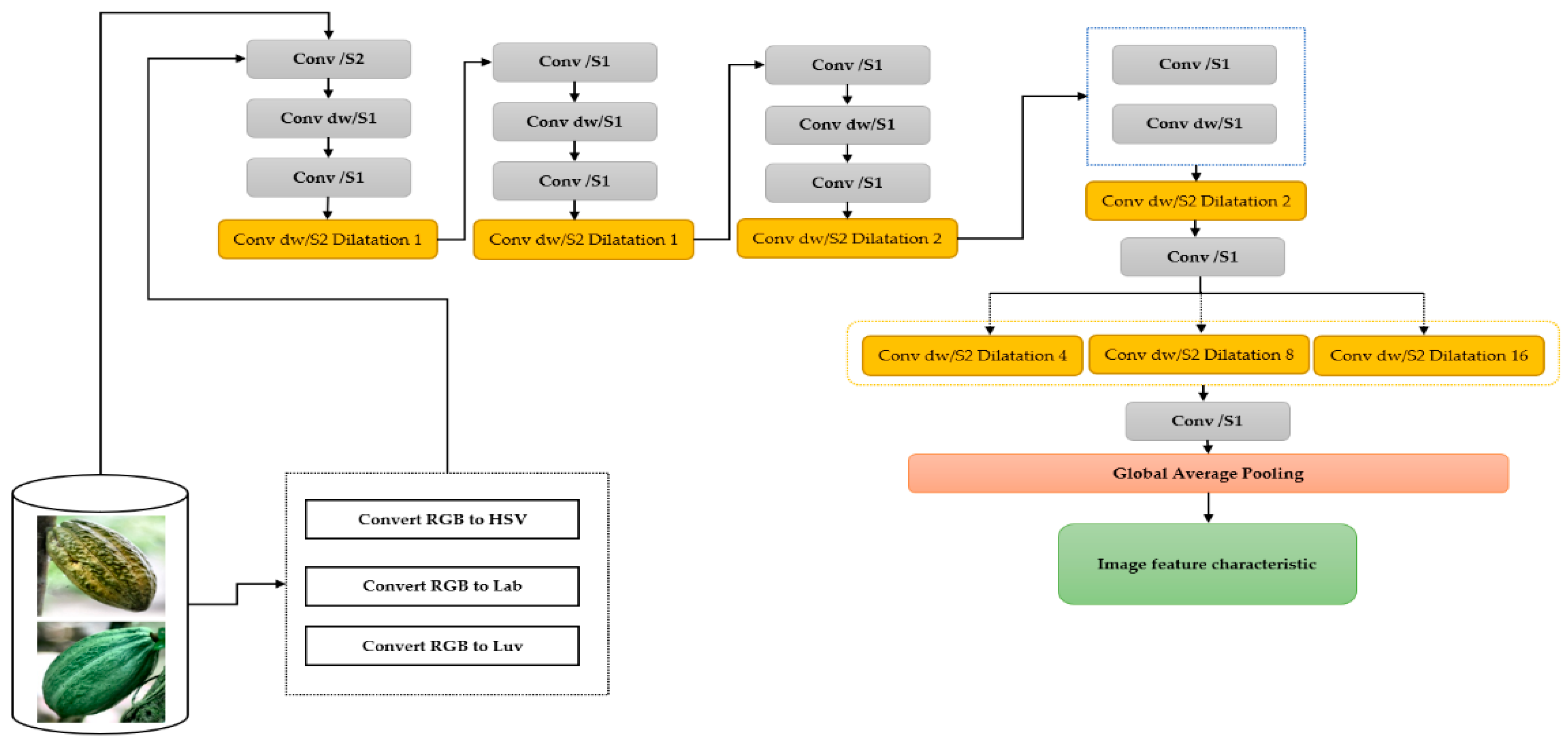
Google developed MobileNet. It is widely used for image classification on mobile devices, object detection, and semantic segmentation [40]. Our study will focus on the convolution part to extract the features. Figure 6 shows the CNN–MobileNet-based retrieval.

Figure 6 depicts the MobileNet CNN-based image feature extraction diagram and follows the following steps:

Step 1: For each image in the database, it is provided as input to the MobileNet convolutional neural network.

Step 2: The input image is then passed through several convolution layers, where filters are applied to extract important features. Batch normalization is performed after each convolution layer to improve generalization and speed up convergence. An activation function is also used for the outputs of the convolution layer to introduce nonlinearity.

Step 3: A layer of Global Average Pooling is added to reduce the dimensionality of the image while preserving important features. The features of the image are then extracted.

3.4. Similarity Measurement Tools

The similarity measure is a mathematical measure used to quantify the similarity or difference between two items in a set of data. It is a crucial element in classification methods based on similarity measures because it allows data grouping according to similarity criteria. The similarity measure is based either on specific characteristics of the data, such as attributes or numeric variables, or it can be based on the similarity between the data profiles [41]. There are several mathematical tools for measuring similarity, and we will use in our study the Euclidean distance, the correlation distance, and the chi-square distance.

3.4.1. Euclidean Distance

The Euclidean distance, also known as the Euclidean norm, is a commonly used measure of distance in geometry, numerical analysis, and statistics. It measures the distance between two points in an n-dimensional Euclidean space, where n is a positive integer [42]. In other words, the Euclidean distance is the length of the straight line that connects two points in space. The Euclidean distance equation is:

$$d\left(X,Y\right)=\sqrt{{\displaystyle \sum }_{i=1}^n{\left(x_i-y_i\right)}^2}$$

(6)

The Euclidean distance is often used in machine learning and data classification fields. For example, in data classification, the Euclidean distance can be used to measure the similarity between feature vectors. If the vectors are similar, their Euclidean distance will be small, indicating that they are closer to each other. If the vectors are very different, their Euclidean distance will be significant, suggesting that they are farther apart.

3.4.2. Correlation Distance

The correlation distance is a measure of the similarity between two random variables. It was introduced in 2005 by Székely and Rizzo as an alternative to the so-called Euclidean distance [43]. Unlike the latter, which is based on the differences between the values of the variables, the correlation distance is based on the correlation between the variables. It is also defined as the correlation between the ranks of the variables [44]. In other words, it measures the similarity between the positions of the values of the two variables. This definition is based on rank theory, which states that the correlation between ranks is independent of the underlying probability distribution. This property is essential because it allows the correlation distance to be used to measure the similarity between variables whose distributions are not known or are not expected. The correlation distance is used to measure the similarity between continuous or discrete variables and is particularly useful when the variables are not linearly related. It is also used to measure the distance between datasets. The following equation defines the correlation distance between the variables X and Y:

$$dC\left(X,Y\right)=1-\frac{\left(x-\overline{x}\right).\left(y-\overline{y}\right)}{{\left|\left|x-\overline{x}\right|\right|}_2{\left|\left|y-\overline{y}\right|\right|}_2}$$

(7)

$\overline{x} \mathrm{and} \overline{y}$ represent the means of x and y respectively.

3.4.3. Chi-Square Distance

The chi-square distance, also known as chi-square distance, is a statistical measure of the similarity or dissimilarity between two datasets. This measurement is based on a comparison between the observed and expected frequencies in a contingency table [45]. It can be used in various fields, such as biology, medicine, sociology, psychology, economics, etc. The concept of the chi-square distance is based on the chi-square distribution, a probability distribution used in tests of independence and goodness-of-fit. This distribution is obtained by summing the squares of the deviations between the observed frequencies and the expected frequencies divided by the desired frequencies [46]. The chi-square distance formula uses this same method to calculate the distance between two datasets.

Calculating the chi-square distance requires two sets of data [47], which can be represented as contingency tables. Each dataset should be divided into categories or classes, and the observed frequencies of each type should be compared to the expected frequencies. Expected frequencies can be calculated from various methods, such as the marginal proportions method, probability distribution method, equidistributional method, etc. Once the observed and expected frequencies have been calculated for each category, the chi-square distance can be calculated using the following formula:

$$X^2=\frac{1}{2}{\displaystyle \sum }_{i=1}^n\frac{{\left(x_i-y_i\right)}^2}{\left(x_i+y_i\right)}$$

(8)

The higher the chi-square distance, the more different the datasets. If the chi-square distance is zero, the datasets are identical. The chi-squared distance value can also be compared to a chi-squared probability distribution to determine the statistical significance of the difference between datasets [48].

3.5. Architecture of the Methodology

Our cocoa pod analysis methodology follows a rigorous six-step process to ensure the accurate classification of mature and unripe pods.

• The first step is to acquire images of cocoa pods for our dataset. We have documented this step in detail in Section 3.1.1 to ensure image quality and consistency.
• In the second step, we perform preprocessing on our data to improve their quality and facilitate their analysis. This step includes the application of the CLAHE algorithm to enhance the contrast of the images, the labeling of the images to reduce their identification, and the extraction and augmentation of the data to increase the size of our dataset. We explained these steps in detail in Section 3.1.2 and Section 3.1.3.
• In the third step, we convert our images to HSV, Lab, and Luv color spaces, which allows us to analyze the colors and shades of the pods more accurately. We presented this step in detail in Section 3.4.
• The fourth step is to extract features from the images using the MobileNet CNN in Section 3.5 and the GLCM in Section 3.6. We chose these two feature extraction techniques to maximize the accuracy of our classification.
• In the fifth step, we divide our data into two parts, one containing the elements characterizing the mature pods and the other containing the elements characterizing the non-mature pods. This step allows us to better understand the distinctive characteristics of the two types of pods.
• Finally, in the sixth step, we use similarity algorithms to measure the similarities between the test data and the essential characteristics of each type of maturity. We then perform the classification using these results. This step is crucial to ensure the accuracy of our final classification.

Our cocoa pod analysis methodology is rigorous and based on proven techniques to ensure the accurate and reliable classification of mature and unripe pods. Figure 7 summarizes the methodology described above:

When a new image is submitted to the database, the parameter extraction process starts. We then classify it and add it to the relevant database.

3.6. Performance Metric

To evaluate the performance of the models in our study, we will use different evaluation metrics, namely accuracy, precision, mean square error, recall, the F1 score, the Matthews Correlation Coefficient, and the ROC curve. They are calculated from the following formulas:

Accuracy is a performance measure that shows how correctly the system has classified the data into the correct class.

$$Accuracy=\frac{TP+TN}{TP+FP+TN+FN}$$

(9)

Precision is the ratio of correctly classified positive images to the total number of genuinely positive images.

$$Precison=\frac{TP}{TP+FP}$$

(10)

Recall is the ability of a classifier to determine actual positive results.

$$Recall=\frac{TP}{TP+FN}$$

(11)

The F1 score is the weighted average of precision and recall.

$$F1 score=2\ast \frac{Precision\ast Recall}{Precision+Recall}$$

(12)

The Matthews correlation coefficient (MCC) is used in machine learning as a measure of the quality of classifications.

$$MCC=\frac{TP\ast TN-FP\ast FN}{\sqrt{\left(TP+FP\right)\left(TP+FN\right)\left(TN+FP\right)\left(TN+FN\right)}}$$

(13)

An estimator’s root means square error measures the mean squared error, i.e., the root means square difference between the estimated and actual values.

$$MSE=\frac{1}{n } {\displaystyle \sum }_{i=1}^n{(Yi-\widehat{Y}i)}^2$$

(14)

The different variables used above are:

• True positives (TP): Images with an actual label that have been classified correctly.
• False positives (FP): Images with an incorrect label that have been classified as positive.
• True negatives (TN): Images with a fake label that have been classified as negative.
• False negatives (FN): Images with an actual label that have been classified as negative.
• Yi: The actual data from the dataset.
• $\widehat{Y}i$: The predicted data from the dataset.

We used the ROC curve, which makes it possible to describe the performance of a model through two indicators; in this case, sensitivity and specificity. It also allows visual verification of performance; it is an essential evaluation measure to verify any model’s effectiveness.

4. Results and Discussion

In this part of our study, we will present the results obtained from the various experiments carried out and the resulting discussions. We have organized this presentation according to the colorimetric spaces studied to highlight their influence on the feature extractors and the results of similarity measures for classification.

We will present the results of each metric for each experiment in tabular form, and we will also represent the confusion matrices and ROC curves. Confusion matrices are an essential tool to assess the accuracy of our classification model by comparing predictions with actual results. The ROC curves, on the other hand, allow us to measure the ability of our model to discriminate between the two classes (mature and non-mature pods). The black dotted line of the ROC curve, also known as the reference line or random line, represents the scenario where the classification model has random or pure random performance. This line represents the lack of discrimination ability of the model and is used as a reference to evaluate the performance of other models. It represents the worst possible scenario, where the model provides no valuable information for classification.

We will also take the time to analyze in detail the results obtained, highlighting the strengths and limitations of each color space. This in-depth analysis is critical to understanding the nuances and complexities of our classification model.

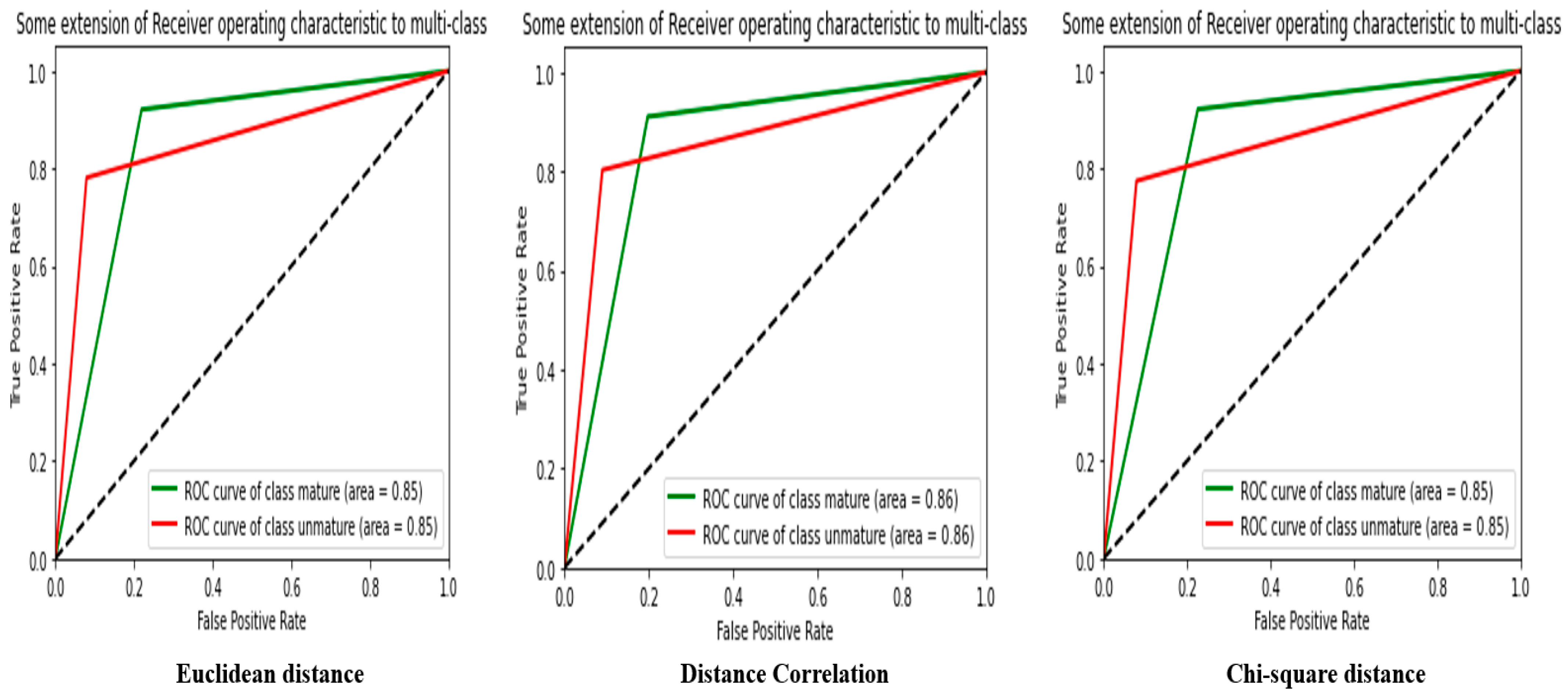
4.1. RGB

Table 1. Evaluation of the performance of algorithms in RGB with the CNN–MobileNet.

Feature Extraction: CNN–MobileNet
Similarity Measure	Accuracy (%)	Precision (%)	MSE	F-Score (%)	Recall (%)	MCC (%)
Euclidean distance	89.94	89.94	0.1002	89.94	89.97	80.35
Distance Correlation	91.21	91.21	0.0877	91.21	91.22	82.65
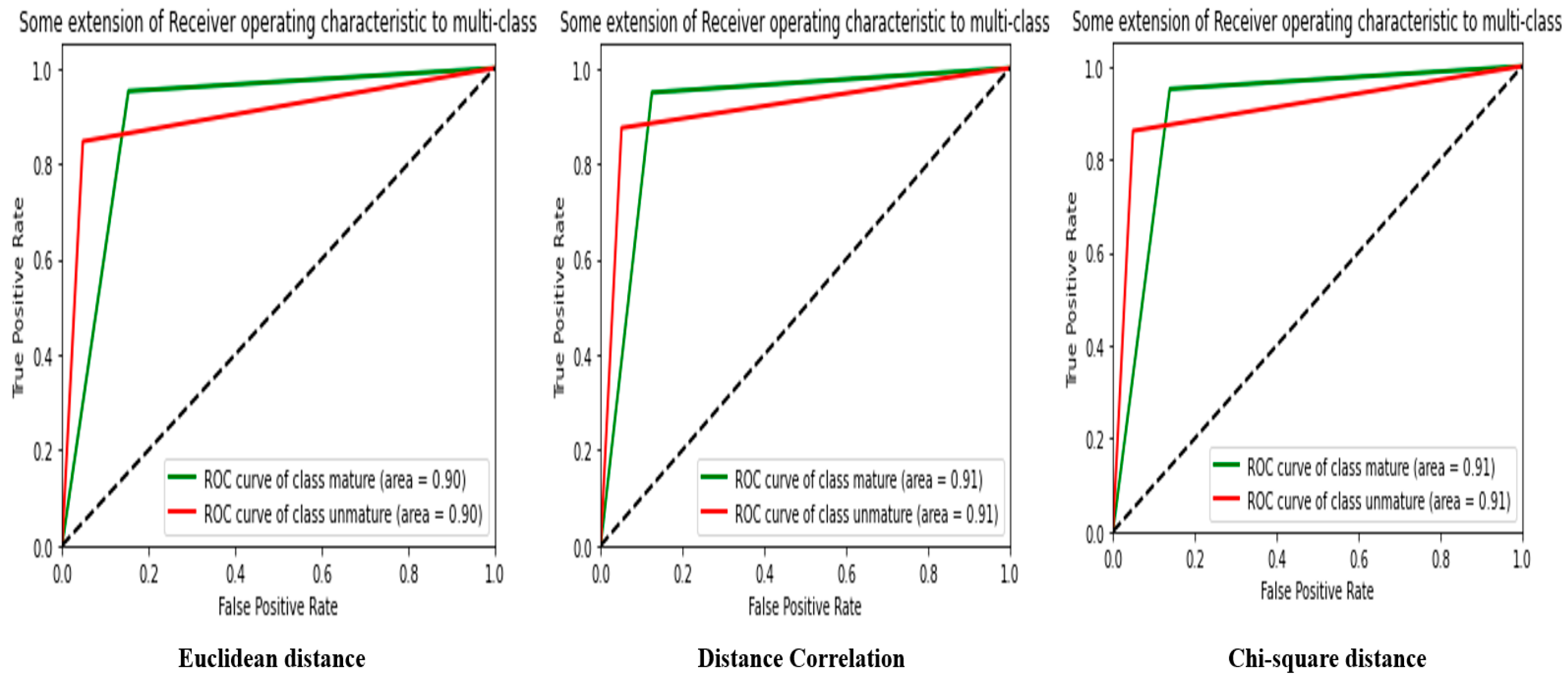
Chi-square distance	90.63	90.63	0.0934	90.63	90.65	81.60

gives the results of the similarity analysis performed using different distance measures on a CNN–MobileNet feature extraction model. Each similarity measure was evaluated in terms of accuracy, precision, root mean square error, F1 score, recall, and Matthews Correlation.

The similarity measure used can have a significant influence on the overall performance of the model. In this case, the Distance Correlation performed best for all metrics evaluated, with an accuracy of 91.21%, a precision of 91.21%, an MSE of 0.0877, an F1-score of 91.22%, a recall of 82.65%, and an MCC of 82.65%. The Distance Correlation is the most efficient way to determine the similarity between the features extracted by the CNN–MobileNet.

The Euclidean distance and chi-square distance measurements also produced similar results, with scores between 89.94% and 90.63%. This indicates that although the choice of similarity measure may influence model performance, the observed differences may be negligible in practice.

Overall, Table 1 shows that the CNN–MobileNet is an efficient model for feature extraction and that the Distance Correlation is an efficient similarity measure to assess the similarity between the extracted features. Figure 8 presents the ROC curve from Table 1.

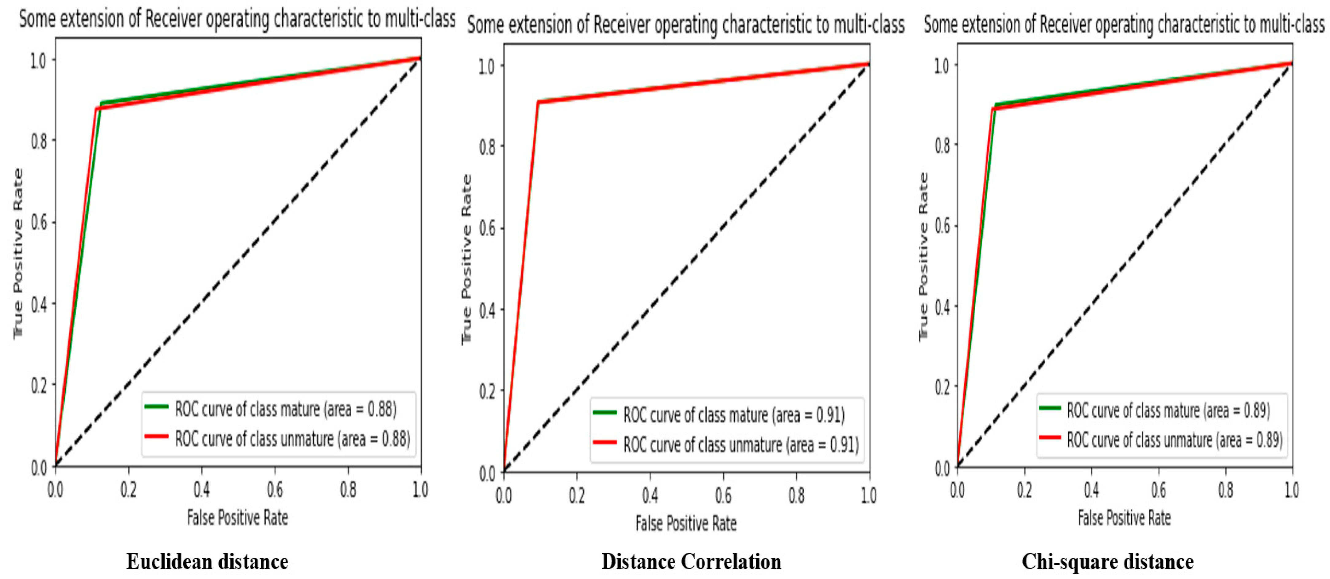
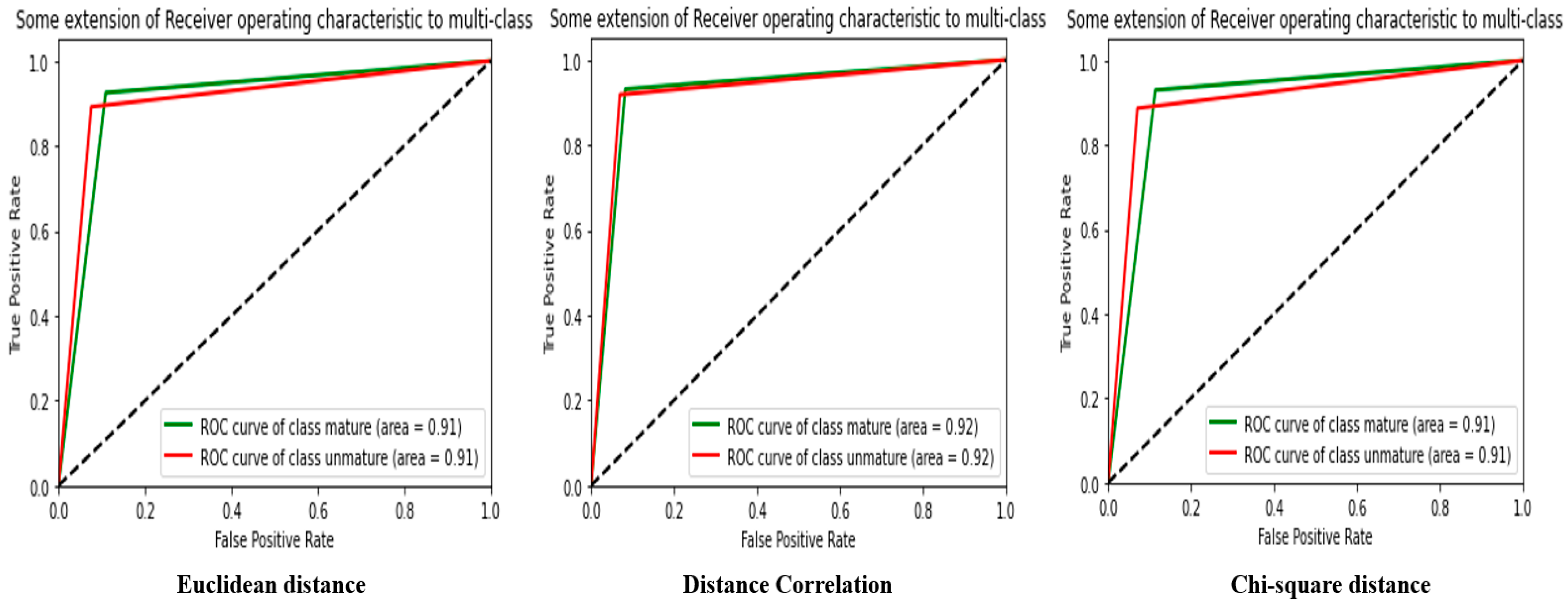
The results of image classification in RGB space with the GLCM extractor are shown in

Table 2. Evaluation of the performance of algorithms in RGB with the GLCM.

Feature Extraction: GLCM
Similarity Measure	Accuracy (%)	Precision (%)	MSE	F-Score (%)	Recall (%)	MCC (%)
Euclidean distance	88.18	88.18	0.1181	88.18	88.18	76.56
Distance Correlation	90.58	90.58	0.0941	90.58	90.58	81.16
Chi-square distance	89.11	89.11	0.1088	89.11	89.11	78.22

, using three different distance measures: the Euclidean distance, correlation distance, and chi-square distance. First, the Euclidean distance results show an accuracy of 88.18%, an MSE of 0.1181, an F-score of 88.18%, a recall of 88.18%, and an MCC of 76.56%. These results indicate that this distance measurement is effective but can be improved to obtain more accurate results. Secondly, the results of the correlation distance show an accuracy of 90.58%, an MSE of 0.0941, an F-score of 90.58%, a recall of 90.58%, and an MCC of 81.6%. These results indicate that the correlation distance is more efficient than the Euclidean distance to classify images in RGB space with the GLCM extractor.

Finally, the results of the chi-square distance show an accuracy of 89.11%, an MSE of 0.1088, an F-score of 89.11%, a recall of 89.11%, and an MCC of 78.22%. These results indicate that the chi-square distance also works well to classify images in RGB space with the GLCM extractor, but it performs slightly worse than the correlation distance.

The analysis of the results shows that the correlation distance measurement is the most effective for classifying images in the RGB space with the GLCM extractor. However, the chi-square distance also works well and can be used as an alternative to the correlation distance depending on the specific classification needs. Furthermore, it is essential to note that the efficiency of each distance measurement also depends on the characteristics of the images to be classified and the complexity of the classification task. Figure 9 shows the ROC curve from Table 2.

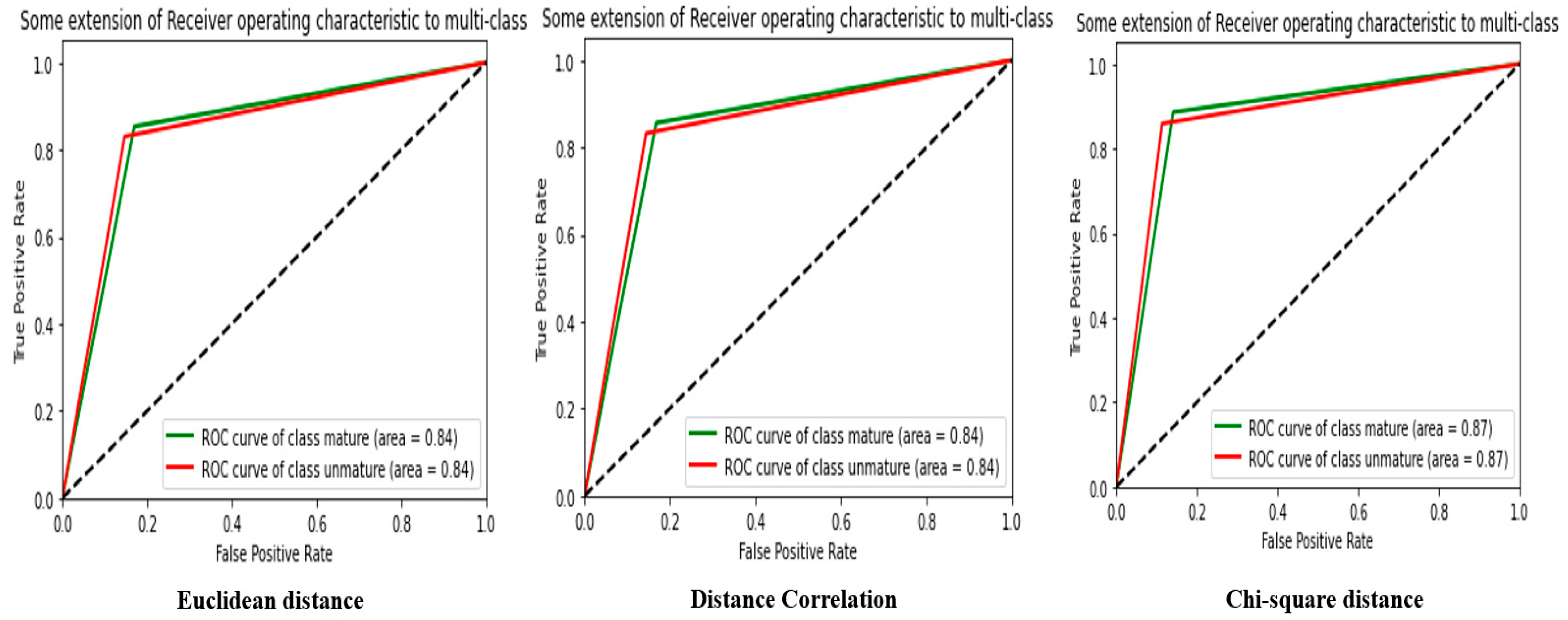
4.2. HSV

Analysis of the results obtained from

Table 3. Evaluation of the performance of algorithms in HSV with the CNN–MobileNet.

Feature Extraction: CNN–MobileNet
Similarity Measure	Accuracy (%)	Precision (%)	MSE	F-Score (%)	Recall (%)	MCC (%)
Euclidean distance	85.06	85.06	0.1485	85.06	85.14	70.90
Distance Correlation	85.63	85.63	0.1432	85.63	85.67	71.71
Chi-square distance	84.76	84.76	0.1514	84.76	84.85	70.39

with MobileNet’s CNN extractor in HSV space and using different distance measures shows that the accuracy of the similarity measure between images can vary depending on the distance measure chosen.

First, using the Euclidean distance to measure the distance between images, we obtained an accuracy, F-score, and MCC of around 85%, which is relatively high. This shows that the Euclidean distance can be a suitable distance metric for measuring the similarity between images in HSV space, although the other distance metrics also have comparable results.

Then, using the Distance Correlation to measure the distance between the images, we obtained slightly better results than those obtained with the Euclidean distance. Accuracy, F-score, and MCC are all over 85%. This shows that Correlation Distance can be a more accurate metric for measuring the similarity between images in HSV space than the Euclidean distance.

Finally, using the chi-square distance to measure the distance between images, we obtained slightly lower results than those obtained with the other distance measures. Accuracy, F-score, and MCC are all below 85%. The chi-square distance may be less accurate for measuring the similarity between images in HSV space.

In terms of MSE, the three distance measurements have comparable values and show that MobileNet’s CNN extractor can capture important image features in HSV space.

Overall, analysis of the results shows that MobileNet’s CNN Extractor can be used to extract features from images in HSV space, and the Distance Correlation is the most accurate distance metric to measure the similarity between the images as the Euclidean distance and the chi-square distance. However, it should be noted that these results were obtained from a specific dataset, and that other datasets may yield different results. Figure 10 shows the ROC curve from Table 3.

Table 4. Evaluation of the performance of algorithms in HSV with the GLCM.

Feature Extraction: GLCM
Similarity Measure	Accuracy (%)	Precision (%)	MSE	F-Score (%)	Recall (%)	MCC (%)
Euclidean distance	84.17	84.17	0.1582	84.17	84.17	68.35
Distance Correlation	84.42	84.42	0.1432	84.42	84.42	68.85
Chi-square distance	87.25	87.25	0.1274	87.25	87.25	74.52

provides the results of using three different distances to evaluate the performance of the GLCM extractor in image classification.

First, the Euclidean distance results show an accuracy of 84.17%, an MSE of 0.1582, an F-score of 84.17%, a recall of 84.17%, and an MCC of 68.35%. These results indicate that the Euclidean distance is relatively accurate in classifying images but may have difficulty distinguishing similar images.

Then, the results of the correlation distance give an accuracy of 84.42%, an MSE of 0.1432, an F-score of 84.42%, a recall of 84.42%, and an MCC of 68.85%. These results are similar to those of the Euclidean distance, suggesting that the correlation distance can be used as an effective alternative to the Euclidean distance.

Finally, the chi-square distance results yielded an accuracy of 87.25%, an MSE of 0.1274, an F-score of 87.25%, a recall of 87.25%, and an MCC of 74.52%. These results are the best among the three distances used and show that the chi-square distance is the most effective in distinguishing similar images.

Analysis of the results in HSV space with the GLCM extractor shows that the chi-square distance is the most efficient for image classification. However, correlation distance can also be an effective alternative to the Euclidean distance. The results of this analysis help guide the choice of the appropriate distance for a specific image classification task. Figure 11 shows the ROC curve from Table 4.

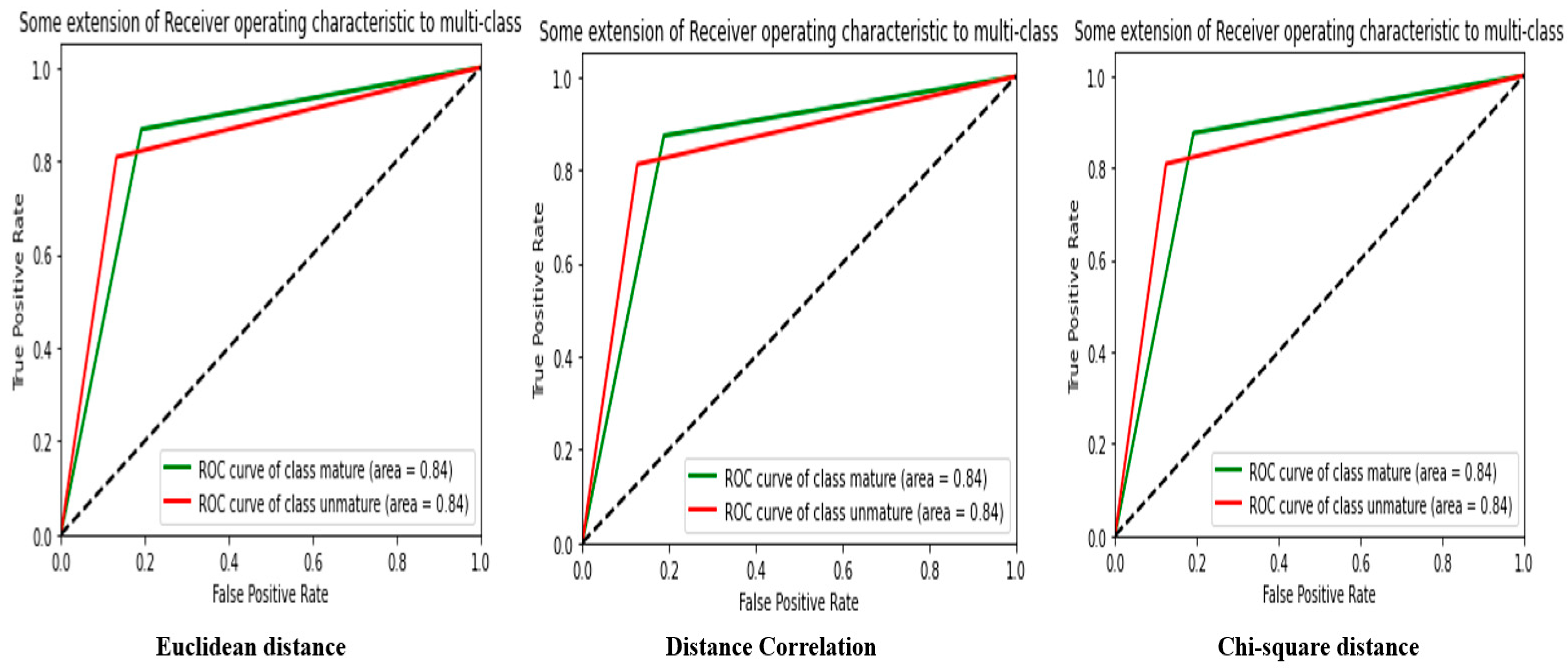
4.3. Luv

Analysis of the results in

Table 5. Evaluation of the performance of algorithms in Luv with the CNN–MobileNet.

Feature Extraction: CNN–MobileNet
Similarity Measure	Accuracy (%)	Precision (%)	MSE	F-Score (%)	Recall (%)	MCC (%)
Euclidean distance	83.79	83.79	0.1618	83.79	83.81	67.71
Distance Correlation	84.26	84.26	0.1571	84.26	84.28	68.65
Chi-square distance	84.18	84.18	0.1578	84.18	84.21	68.53

shows that MobileNet’s CNN feature extractor can provide relatively high image classification performance in Luv space, with an average accuracy of 84%.

The Euclidean distance measurement gave an accuracy of 83.79%, which is slightly lower than that of the Distance Correlation and the chi-square distance. The Distance Correlation accuracy was the highest, with an accuracy of 84.26%, followed closely by the chi-square distance, with an accuracy of 84.18%.

For accuracy, all three distance measurements gave very close results; this means that features extracted by MobileNet’s CNN feature extractor are distinct enough in Luv space to allow for accurate image classification.

The F-score, which combines precision and recall, is also high for all three distance measures, with an average accuracy of 84.09%. Recall was slightly higher for the Distance Correlation measure, which scored 68.65%.

For the mean square error (MSE), the Distance Correlation measure gave the lowest value, 0.1571, while the chi-square distance gave the highest value, 0.1578. This means that the Distance Correlation measure can be more accurate in assessing the model’s classification performance.

Finally, the Matthews Correlation Coefficient (MCC) gave relative values for all three distance measures, with the Distance Correlation measure giving the highest value at 68.53%.

In sum, analysis of the results shows that MobileNet’s CNN feature extractor provides high image classification performance in Luv space, with similar performance for the Euclidean distance, Distance Correlation, and chi-square distance. The Distance Correlation measure is, however, slightly more accurate in assessing the model’s classification performance. Figure 12 shows the confusion matrix and ROC curve from Table 5.

Table 6. Evaluation of the performance of algorithms in Luv with the GLCM.

Feature Extraction: GLCM
Similarity Measure	Accuracy (%)	Precision (%)	MSE	F-Score (%)	Recall (%)	MCC (%)
Euclidean distance	83.60	83.60	0.1639	83.60	83.60	67.20
Distance Correlation	86.93	86.93	0.1306	86.93	86.93	73.86
Chi-square distance	90.76	90.76	0.0923	90.76	90.76	81.52

provides results for the similarity analysis of features extracted from the GLCM in Luv space using similarity measures. Results are given for three different similarity measures: the Euclidean distance, the correlation distance, and the chi-square distance.

The table shows that the best-performing similarity measure is the chi-square distance, with an accuracy rate of 90.76% and an MSE value of 0.0923. The correlation distance is the second-best performing similarity measure, with an accuracy rate of 86.93% and an MSE value of 0.1306. The Euclidean distance is the worst-performing similarity measure, with an accuracy rate of 83.60% and an MSE value of 0.1639.

It is important to note that the precision, F-score, recall, and MCC for each similarity measure is equal to the precision rate.

These results show that the best-performing similarity measure for the analysis of features extracted from the Luv space is the chi-square distance, closely followed by the correlation distance. The Euclidean distance is the worst-performing similarity measure. These results can help choose the appropriate similarity measure for classification and pattern recognition tasks involving the Luv space. However, it should be noted that performance may vary depending on the characteristics of the dataset and the purposes of the analysis. Figure 13 presents the confusion matrix and the curve ROC from Table 6.

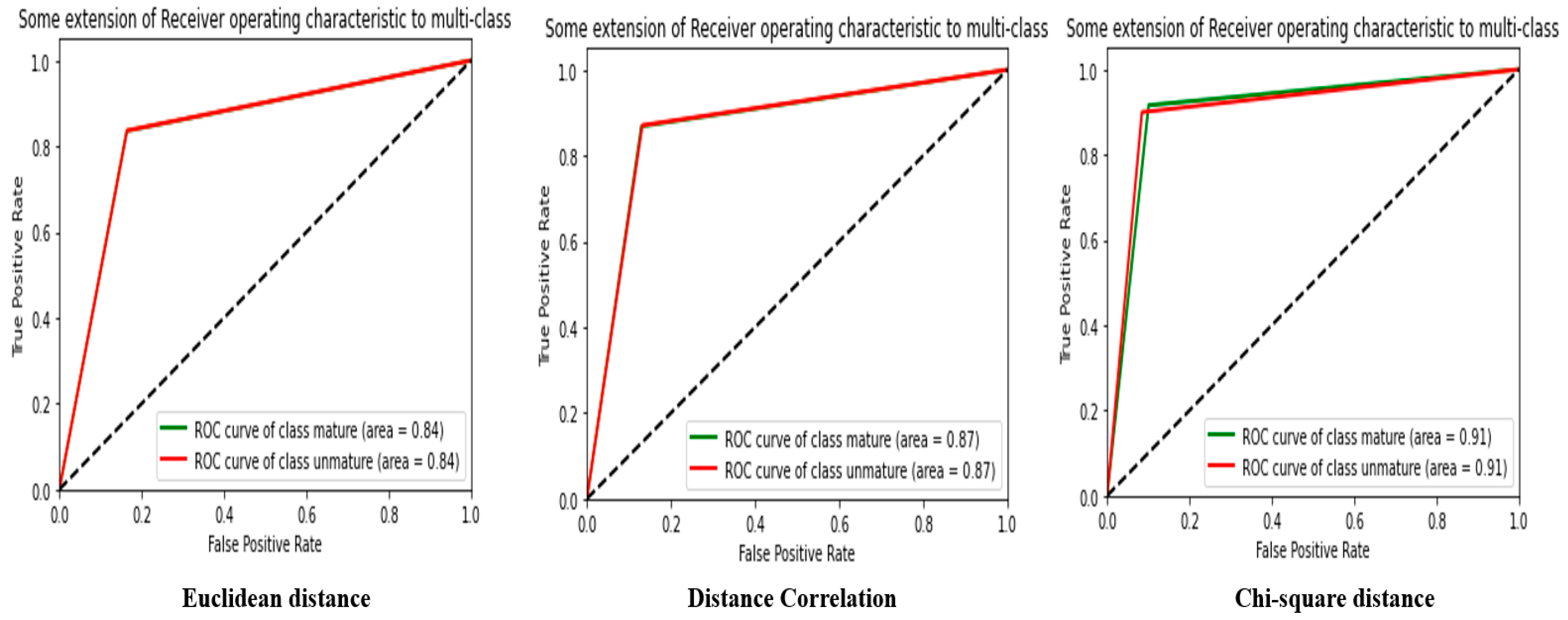
4.4. Lab

In

Table 7. Evaluation of the performance of algorithms in Lab with the CNN–MobileNet.

Feature Extraction: CNN–MobileNet
Similarity Measure	Accuracy (%)	Precision (%)	MSE	F-Score (%)	Recall (%)	MCC (%)
Euclidean distance	90.83	90.83	0.0916	90.83	90.83	81.70
Distance Correlation	92.48	92.48	0.0751	92.48	92.48	84.96
Chi-square distance	90.82	90.82	0.0916	90.82	90.83	81.72

, CNN–MobileNet was used to extract image features from two datasets and to measure the distances between these features using three different distance measurement methods: the Euclidean distance, correlation, and the chi-square distance.

The results show that the correlation distance performed best among the three distance measurement methods. It obtained the best score for accuracy (92.48%), precision (92.48%), F-score (92.48%), and recall (92.48%). In addition, the correlation distance also recorded the lowest root mean square error (MSE) among the three methods.

In contrast, the Euclidean distance and the chi-square distance obtained similar results. They both recorded an accuracy, F-score, and recall of 90.83%, as well as a root mean square error of 0.0916. However, the chi-square distance recorded a slight improvement in precision and recall compared to the Euclidean distance.

The Matthews Correlation of the three methods recorded similar results, with an MCC of 81.70% for the Euclidean distance, 84.96% for the correlation distance, and 81.72% for the chi-square distance.

This analysis shows that the correlation distance is the most effective distance measurement method for image classification using the CNN–MobileNet extractor. However, the Euclidean distance and the chi-square distance can also be used with similar performance, depending on the specific needs of each project. Figure 14 shows the ROC curve from Table 7.

Table 8. Evaluation of the performance of algorithms in Lab with the GLCM.

Feature Extraction: GLCM
Similarity Measure	Accuracy (%)	Precision (%)	MSE	F-Score (%)	Recall (%)	MCC (%)
Euclidean distance	99.39	99.39	0.0060	99.39	99.39	98.70
Distance Correlation	99.31	99.31	0.0068	99.31	99.31	98.64
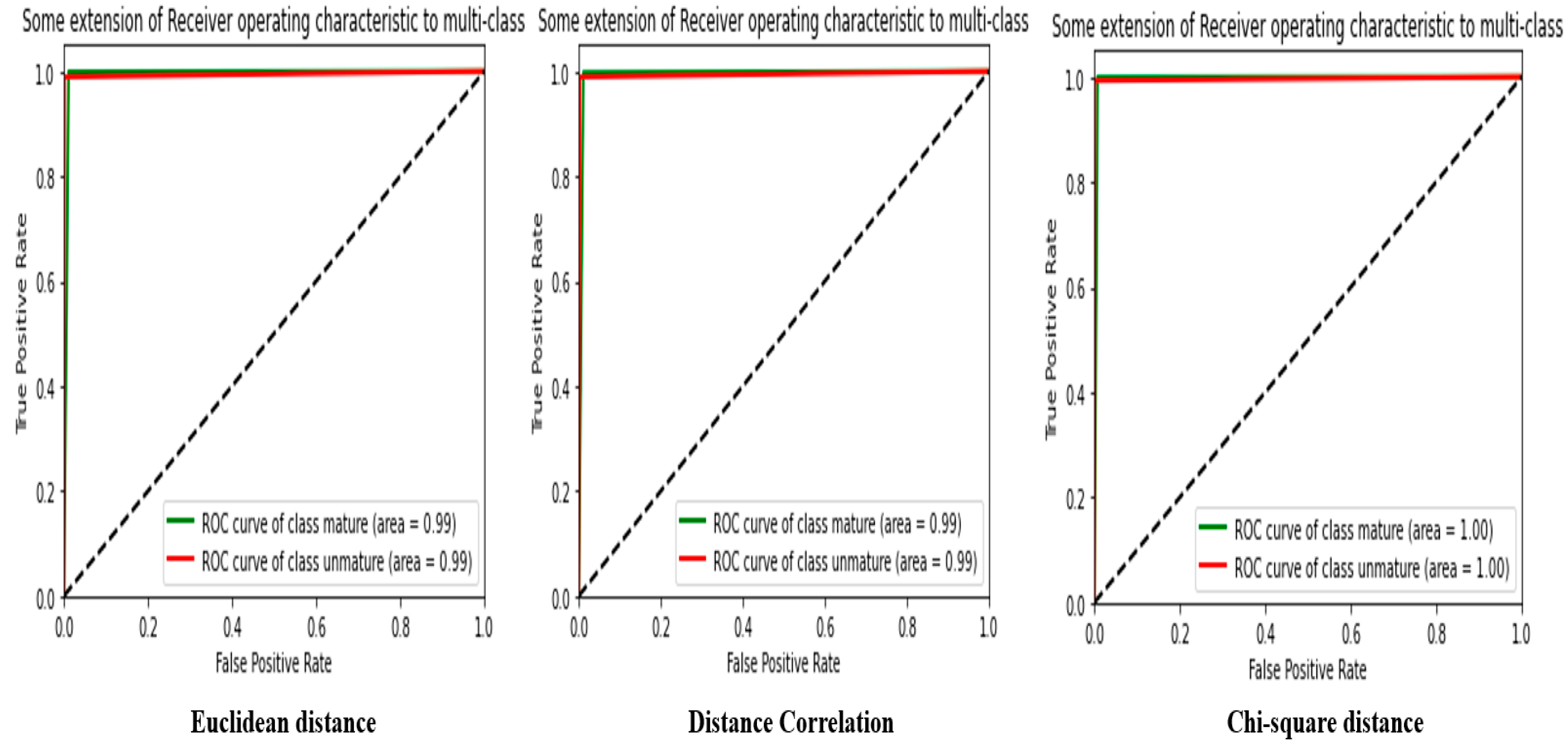
Chi-square distance	99.60	99.60	0.0039	99.60	99.60	99.21

provides an in-depth analysis of different distances measured using the Lab space with the GLCM.

The first similarity measurement was made with the Euclidean distance, which has a precision and accuracy of 99.39%. This means measuring the distance between pixels in Lab space is accurate, with a root mean square error (MSE) of 0.0060. The F-score and recall are also very high, at 99.39% and 98.70%, respectively. The Matthews Correlation Coefficient (MCC) is also very high at 98.70%, indicating a perfect correlation between predicted and actual results.

The second similarity measurement was made with the correlation distance, which has a precision and accuracy of 99.31%. This indicates similar accuracy to the Euclidean distance but with a slight drop in other performance metrics. The MSE is slightly higher at 0.0068, and the F-score and recall are also marginally lower at 99.31% and 98.64%, respectively. The MCC is also slightly lower at 98.64%.

The third distance measured is the chi-square distance, which has the highest precision and accuracy of all measurements, with a value of 99.60%. The MSE is also very low at 0.0039. F-score, recall, and MCC are also very high at 99.60%, 99.60%, and 99.21%, respectively. This indicates that the chi-square distance is the best distance measure for this dataset in Lab space with the GLCM.

We also conducted an in-depth analysis of the distance measurements for the dataset in the Lab space with the GLCM. The chi-square distance is the most precise measurement, with 99.60% precision and accuracy. Other distance measures, such as the Euclidean and correlation distance, are also very accurate, with similar performance, but slightly lower than the chi-square distance. Figure 15 shows the confusion matrix and ROC curve from Table 8.

4.5. Influence of Color Spaces

By observing the color spaces, we noticed their impact on our data and the feature extractors in our study. The corresponding results are shown in

Table 9. Summary table of expected results in different color spaces.

Color Space	Similarity Measure	Feature Extractor	Accuracy (%)
RGB	Distance Correlation	CNN–MobileNet	91.21
RGB	Distance Correlation	GLCM	90.58
HSV	Distance Correlation	CNN–MobileNet	85.63
HSV	Chi-square distance	GLCM	87.25
Luv	Distance Correlation	CNN–MobileNet	84.26
Luv	Chi-square distance	GLCM	90.76
Lab	Distance Correlation	CNN–MobileNet	92.48
Lab	Chi-square distance	GLCM	99.60

.

Table 9 shows the impact of color spaces on the performance of two different feature extractors for image classification tasks.

The results show that the choice of color space, distance measure, and feature extractor can significantly impact the performance of image classification.

First, the color space used can affect classification accuracy. The results show that the Lab space gives the best accuracy results for both feature extractors, while the HSV space gives the weakest results. This may be because the Lab space is designed to be perpetually uniform, while the HSV space is based on polar coordinates and may need to be more easily interpretable for human perception.

Moreover, the choice of the similarity measure can also affect the results. The results show that the Distance Correlation in the RGB and Lab space gives better accuracy results for CNN–MobileNet and GLCM, while the chi-square distance in the HSV space gives better results for GLCM. This may be due to differences in how similarity measures calculate similarities between image features.

Finally, the choice of feature extractor can also impact classification performance. The results show that the two feature extractors have different performances according to the color spaces and the distance measurements. Ultimately, these results highlight the importance of considering the choice of color space, distance measure, and feature extractor to obtain the best image classification results. This can be particularly important for computer vision applications where accurate classification performance can be critical.

4.6. Comparison with Existing Methods

The results obtained in our study are particularly remarkable. The scores we obtained are fascinating and surpass those reported in the literature, as shown in

Table 10. Comparison of the best scores of our methods with methods from the literature.

Models	Accuracy (%)
Oliveira et al. [17]	90.00
Lab—CNN–MobileNet—Distance Correlation	92.48
Bueno et al. [16]	97.46
Lab—GLCM—Chi-square distance	99.60

. These results attest to the effectiveness of the methodology we used and the quality of our dataset.

However, it is essential to note that some limitations should be considered when interpreting these results.

Oliveira et al. [17] used the Inception-ResNet-V2 model to detect cocoa pod ripeness, which was trained on an extensive image database and successfully used for different image recognition tasks. By using transfer learning with this model, it is possible to benefit from its performance to solve an image recognition task without needing the same amount of data or computation time. However, this pre-trained model may not be suitable for the target task and may need to be adapted by adjusting some model layers or adding new layers. Furthermore, there are often differences between the data used to train the pre-trained model and the target data; this can affect the performance of the trained model.

Bueno et al. [16] used a technique that uses audio data from the exocarp (outer part) of the cocoa pod to detect the maturity of cocoa pods. Mel-frequency cepstrum was used to extract recognizable features for the ripening process, and a convolutional neural network was used to classify cocoa pods. This process has yielded satisfactory results, but there are limitations to this technique, so the quality of the recording may influence the accuracy of the data analysis. If the recording could be of better quality, it may be complex to extract reliable information. Additionally, the dataset size (4465 audio files) may be considered a small sample compared to other datasets used in machine learning, which may limit the accuracy of the analysis and the generalization of the results obtained to different samples of cocoa beans.

For our study, we can register limitations of different aspects. First, using convolutional neural networks (CNNs) for feature extraction has several limitations. First, they often require a large amount of training data to operate effectively, which can be challenging to obtain in some situations. Second, they are complex and computationally intensive to train and use. Finally, they can be sensitive to variations in lighting and other image disturbances, which can affect their performance. GLCM (gray-level co-occurrence matrix) texture extractor is a technique for extracting texture features from an image by measuring how often different levels of gray appear together in the image. This approach may help to remove texture features robustly but may be less effective in extracting more complex characteristics, such as shapes or patterns.

5. Conclusions

This in-depth study focused on evaluating the efficiency of feature extractors and the influence of color spaces on these extractors for the classification of cocoa pod maturity from images in our database. Several similarity measures were used in conjunction with feature extractors to classify the pod images according to their level of maturity. Classification performance was examined from different angles using feature extractors based on convolutional neural networks (CNN) and gray-level co-occurrence matrix (GLCM) on other color spaces, such as RGB, HSV, Lab, and Luv. The results showed that the Lab color space using GLCM and the chi-square distance similarity measure produced the best results, with an accuracy of 99.60%. The use of artificial intelligence for detecting cocoa pod maturity can offer many advantages for future studies. To enrich our database, we plan to add images of cocoa pods at all stages of their development, from their appearance on the tree to their harvest. This initiative will help improve our understanding of the growth and evolution of these pods and allow us to prevent diseases that could harm the crop.