A Set of Geophysical Fields for Modeling of the Lithosphere Structure and Dynamics in the Russian Arctic Zone

Abstract

This paper presents a set of various geological and geophysical data for the Arctic zone, including some detailed models for the eastern part of the Russian Arctic zone. This hard-to-access territory has a complex geological structure, which is poorly studied by direct geophysical methods. Therefore, these data can be used in an integrative analysis for different purposes. These are the gravity field, heat flow, and various seismic tomography models. The gravity field data include several reductions calculated during our preceding studies, which are more appropriate for the study of the Earth’s interiors than the initial free air anomalies. Specifically, these are the Bouguer, isostatic, and decompensative gravity anomalies. A surface heat flow map included in the dataset is based on a joint inversion of multiple geophysical data constrained by the observations from the International Heat Flow Commission catalog. Available seismic tomography models were analyzed to select the best one for further investigation. We provide the models for the sedimentary cover and the Moho depth, which are significantly improved compared to the existing ones. The database provides a basis for qualitative and quantitative analysis of the region.

Dataset: http://www.wdcb.ru/arctic_antarctic/arctic_geoph.fields.html.

Dataset License: CC-BY-NC

1. Summary

1.1. Overview

The structure of the lithosphere and the variations of its density, thickness, sedimentary cover, geothermal heat flow, and other physical properties are directly related to its geological history and the main forces that drive the tectonic processes. The Circumpolar Arctic, including the Russian Arctic zone, is still one of the least studied territories due to its poor accessibility. The details of the geological history of particular tectonic units, as well as of some geological structures located in this region, are still unknown or inconsistent as they are based on outdated results. Geological studies of the Arctic zone using operational data models based on geophysical data from modern satellite missions and ground-based surveys can help to improve the knowledge of the tectonic history of the region.

Another factor that determines the need to study the lithosphere of the Arctic is the importance of prospecting and exploration of mineral deposits. For example, the Russian Arctic zone area is known for its high mineral resource potential [1]. There exist significant ore-placer areas (Severo-Yansky in Yakutia and Pyrkakaysky at the Chukotka peninsula), as well as nickel (Oktyabrsk and Talnakh), zinc (Pavlovsk), lead (Taimyr Peninsula), copper (Norilsk ore region), molybdenum (Circum-Arctic zone), and tin deposits (Lyakhovsky Island and Chukotka). Gold and silver deposits are distributed in the Arctic zone in Chukotka and Yakutia. Furthermore, it should be noted that the distribution of rare metals is confined to the Kola Peninsula, and one of the largest deposits, Tomtorskoye, is also located in Yakutia [2,3]. Since the area is large, not all potential deposits have been discovered yet. This gives reason for a more detailed study of the whole region. Gas and oil deposits are also common in the Arctic zone. The majority of deposits (which can be developed cheaply and easily) are discovered now, but there are a lot of prospective hard-to-access areas that are not sufficiently studied [4].

The next important issue is global warming, which nowadays is one of the most actual problems on a planetary scale [5]. Its potential impact on the Arctic zone could be very significant since global warming leads to the melting of glaciers and permafrost. Changes in the extent and thickness of permafrost lead to a decrease in the bearing capacity of the soil and deformation of the road constructions [6]. Therefore, due to the degradation or loss of the permafrost, most of the constructions and transport facilities must be completely replaced. It has been recently recognized that the melting process depends not only on climate changes but also on the geothermal heat flow [7,8]. Therefore, only considering both factors provides a possibility to predict the future behavior of the glaciers and permafrost, which is crucially important for all types of constructions in the Arctic zone. This problem remains completely unstudied.

The final factor illustrating the importance of analyzing the geological and geodynamic conditions of the Arctic is seismicity. Today, a large number of studies are being carried out to study seismic hazards, and given the large area, the Arctic region requires constant monitoring of geodynamic conditions [9,10,11]. It is well known that the earthquake distribution is directly related to the structure of the crust and upper mantle; therefore, their parameters should be analyzed together with the direct seismic observations.

Based on the above factors, we can make a general conclusion about the necessity of a detailed study of the lithosphere and geodynamics of the Arctic region. Such studies require various geological and geophysical information contributing to various details of the Arctic lithosphere, its structures, and development. In this paper, we present a collection of geophysical fields which can be used in various studies related to the abovementioned aspects. The dataset includes the results of our previous studies of the Arctic lithosphere and the data derived from publicly free resources; here, we present them as a combined dataset that is freely available and can be downloaded in digital form.

1.2. Geological and Tectonic Background

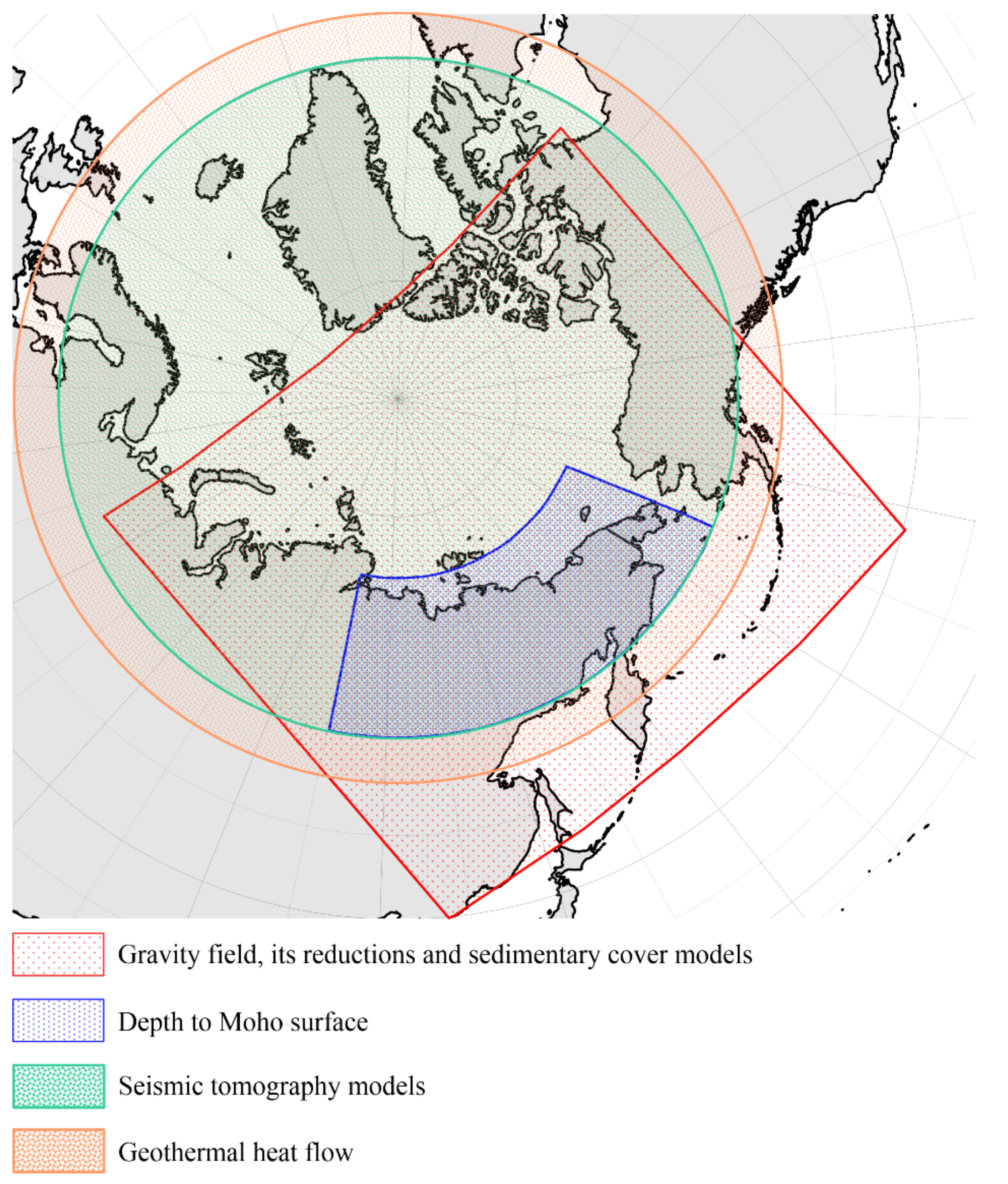
The Arctic region of Russia is characterized by complex tectonic structures that have formed due to various geological processes such as continental collisions, subductions, and extensions. A comprehensive geological and tectonic analysis of this region is beyond the scope of this article; however, a brief overview of its development is provided here, with further details available in [12,13].

In the Precambrian era, the region was a part of the ancient continent of Arctica (Arctida). During this time, the region experienced extensive volcanic activity and the formation of large troughs. The second stage occurred in the Paleozoic era when the region was part of the supercontinent of Pangea. During this time, the region experienced continental collisions and the formation of mountain ranges, such as the Ural Mountains. The third stage occurred in the Mesozoic era. During the destruction of Pangea, the Amerasian Basin opened in the Late Jurassic–Cretaceous. During the fourth, Cenozoic-era stage, the region underwent extensive extensions due to the opening of the Eurasian Basin. This resulted in the formation of large rift basins and the development of offshore oil and gas deposits. These two major basins—Amerasian and Eurasian—form the present Arctic Ocean. The Gakkel Ridge [14] is a continuation of the Mid-Atlantic Ridge. The continuation of the Gakkel Ridge into Asia is the Moma rift—a part of a margin between the North American and Asian tectonic plates [15]. Large volumes of sedimentary rocks reaching a thickness of up to 20 km have accumulated in the passive margins during post-orogenic periods, forming the shelf of the Arctic seas [16]. According to the regional studies of the circumpolar lithosphere [16], there exist two types of oceanic crust in the Arctic zone, five types of continental crust, differing in thickness of the “granite–gneiss” and “basalt” layers, and the crust of a transition type, represented by a local segment within the Amerasian basin.

The most ancient geological structures in the Russian Arctic zone are linked to the cratons of the region. The Fennoscandinavian Shield, which belongs to the East European Craton, constitutes the westernmost section of the Russian Arctic continental zone. The Siberian Craton is another significant craton associated with this area. These two cratons are divided by the Uralian and Taimyr fold belts, which originated during the Late Paleozoic period, as well as by the Pai–Khoi–Novaya Zemlya–South Taimyr fold belt that developed during the Early Mesozoic era. The West Siberian plate, represented by sedimentary rocks on the Hercynian basement that dates to the Middle to Late Paleozoic period, is also located in this area.

The eastern part of the Russian Arctic (Figure 1) is represented by the Verkhoyansk–Chukotka fold–nappe system adjacent to the Siberian Craton, the Okhotsk–Chukotka volcanogenic belt (OCVB), and the Chukotka and Anadyr–Koryak tectonic domains. These large terrains formed due to a sequence of collisions in the Cretaceous [12,17], which, in particular, led to the formation of large mountain belts such as the Chersky and Verkhoyansk Ridges. The Chukotka terrain and the Anadyr–Koryak folded system, located in the easternmost part of the Russian Arctic, formed during the Mesozoic to Cenozoic. The Anadyr–Koryak folded system formed as an accretionary prism of a subduction zone. In the Late Cretaceous, the OCVB formed of the Early to Late Cretaceous terrigenous, volcano–tuff–terrigenous, and volcanic rocks, (rhyolites, andesites, and basalts), extending along the north coast of the Sea of Okhotsk for about 3000 km and then to the northeast in the Chukotsk Peninsula.

To date, this eastern part, including northeastern Asia, is still one of the least studied areas, despite the overall progress in geography and remote sensing. The point is that the appropriate geographical and geological exploration of this region began only about a century ago. Geological studies of the region focused mainly on mineral prospecting, including mostly surface studies. Some of them are still sketchy. The coverage of the region with the results of geophysical methods aimed at studying deep structures (first, seismic methods) remains insufficient. As a result, the geological history of some areas within the region is based on generalized, and sometimes even outdated, hypotheses (in some cases there are even contradicting hypotheses about the origin and development of some areas, such as Chukotka).

All recent studies have demonstrated that any geophysical field cannot be used by itself for the construction of comprehensive models of the crust and upper mantle. For example, the seismic reflection and refraction data, which provide the most detailed images of the crust, are usually distributed very heterogeneously and do not provide full coverage of the study area, as in the northern part of Eurasia [18]. Seismic tomography models provide consistent images of the mantle, but usually with low resolution [19]. Furthermore, variations of seismic velocities could be associated with both thermal and compositional anomalies, for which effects cannot be divided without additional information [20,21]. Heat flow determinations are also very sparse and unevenly distributed. On the other hand, potential fields (gravity and magnetic) are usually characterized by good coverage, but their interpretation represents an ill-posed problem and many alternative models can be constructed, which could be principally different.

Therefore, the common view now is that only an integrative analysis of various geophysical fields can give reliable models of the crust and upper mantle. This is especially true for the Russian Arctic zone, where some geophysical data are missing for large parts.

In this paper, we present a combination of geophysical fields, both obtained during our preceding studies in 2021–2022 and derived from freely accessible resources. The dataset spatial coverage includes not only the eastern part of the Russian Arctic zone, which is only the main study area, but also larger territories and even the Circumpolar Arctic area for the data derived from global models. The presented dataset can be used in the future for the construction of detailed 3D models of the crust and upper mantle in the northern part of Eurasia.

2. Data Description

The gravity field dataset includes the ASCII files and grids for the following fields:

• Bouguer gravity anomalies derived from the EIGEN-6c4 gravity field model;
• Residual Bouguer anomalies;
• Corrected topography for 2.67 g/cm³ (total surface load);
• Map of isostatic correction to the gravitational field;
• Map of isostatic gravity anomalies (mGal) (Figure 2);
• Map of decompensative correction to the gravitational field;
• Map of decompensative gravity anomalies (mGal) (Figure 3).

The ASCII data files have a unified format for gravity data, including the geographic and local coordinates and the mapped field values. The data grids, corresponding to the data and having the same names as the ASCII data files, also have a unified format and are compatible with Arc/Info ASCII grids. A more detailed data format description is provided on the website (see dataset link).

The dataset includes two sedimentary thickness models obtained from the decompensative gravity anomalies (Figure 4 displays the first of these two models; the second one differs in its initial conditions), the density correction map, and the map of the corrected density, averaged vertically. This is a set of the results of the abovementioned approach based on the decompensative gravity anomalies. The data are freely accessible. The study area spans from 135° to 190° E and 65° to 74° N, although the initial area was larger and included 5600 × 5400 km in the orthographic projection with a center point of 162.5° E, 72.5° N. This was performed for a more convenient calculation. The structure of the grids for sedimentary models is similar to the structure of the grids for gravity fields described in the previous subsection.

The Moho depth dataset (mw21-vs-cor.dat) covers a rectangular region of northeastern Eurasia, including the Eastern Russian Arctic segment (60° to 75° N and from 110° to 190° E). The data file contains three columns: the first two are the geographic coordinates (179–170° W longitudes are denoted as 181–190° E for convenience), and the last one is the Moho depth values in km from the sea level. The data spatial resolution is 1° × 1°.

The geothermal heat flow dataset includes an area from 51° to 90° N, covering the whole Arctic, northern Eurasia, and northern North America. The data points have an average spatial step of about 100 km (the latitudinal step is 1°, and the longitudinal step is 2.2°) and are referenced to a local system of rectangular coordinates with a center in the North Geographic Pole. The data file contains five columns: geographical coordinates (latitude, longitude), local coordinates (X, Y from the geographical North Pole), and the heat flow values in mW/m² (see Data Availability Statement section for details provided on the website).

The seismic tomography dataset includes the text data files (for models SL2013sv, S40RTS, and SEMum2) and data grids (for the SMEAN2 model) for the Circumpolar Arctic area (from 60° to 90° N). The data values are velocity anomalies in %. The SL2013sv, S40RTS, and SEMum2 models have a latitudinal step of 0.5° and a longitudinal step of 0.5°. For each model, the data include the depth slices from 0 to 650 km with a step of 50 km (50–650 km for the SL2013sv model). All the ASCII files have a similar format: they contain columns of the geographical longitude, latitude, and S-wave velocity anomaly in %. The SMEAN2 data files have the same structure as the data files from the abovementioned SEMum2, S40RTS, and SL2013sv models. The latitudinal resolution of the SMEAN2 model is higher (the latitudinal step is 5 arc min, which is 0.083°); therefore, the data files for SMEAN2 depth slices are larger than the ones for the other three models.

Therefore, the original datasets obtained during our previous research (gravity field reductions, sedimentary cover, Moho depth, geothermal heat flow) were united with the seismic tomography dataset, which was derived from publicly available models. No extra updates were applied to the existing data. The groups of datasets differ in their spatial coverage. The scheme in Figure 1 shows the details of spatial coverage for the data presented. As seen, the seismic tomography model dataset covers the whole Circumpolar Arctic from 60° N. The geothermal heat flow data are also related to the Circumpolar Arctic, covering the area from 56° northward. The area selected for gravity reductions and sedimentary cover models is close to a square covering most of the Arctic basin and Northern Eurasia. Finally, the Moho data cover an area of 135° E to 190° E and 60° N to 75° N.

3. Methods and Results

3.1. Main Reductions of the Gravity Field in Northeastern Eurasia

Density anomalies within the Earth, which are reflected in the observed gravity field, are crucially important for understanding the structure and tectonics of the lithosphere and upper mantle. First of all, density differentiation represents the driving force for all tectonic processes since it stimulates the movement of the material within the Earth [22]. On the other hand, these processes lead to concentration of the density anomalies in the upper lithosphere which are responsible for strong stresses and, consequently, for seismicity [23]. Therefore, the knowledge of the density variations within the crust and upper mantle is important for many geophysical implications [24].

Another important advantage of the gravity field is that, contrary to most other geophysical data, it gives homogeneous coverage for most areas. This is especially important for the eastern part of the Russian Arctic zone, where other geophysical determinations are extremely sparse. Recent satellite missions (chiefly, GRACE and GOCE) have provided, together with ground observations, for the first time, a possibility to create homogeneous high-resolution gravity field models for nearly the whole of Earth. Here, the model EIGEN-6c4 [25] has been used to calculate the Bouguer, isostatic, and decompensative gravity anomalies [26].

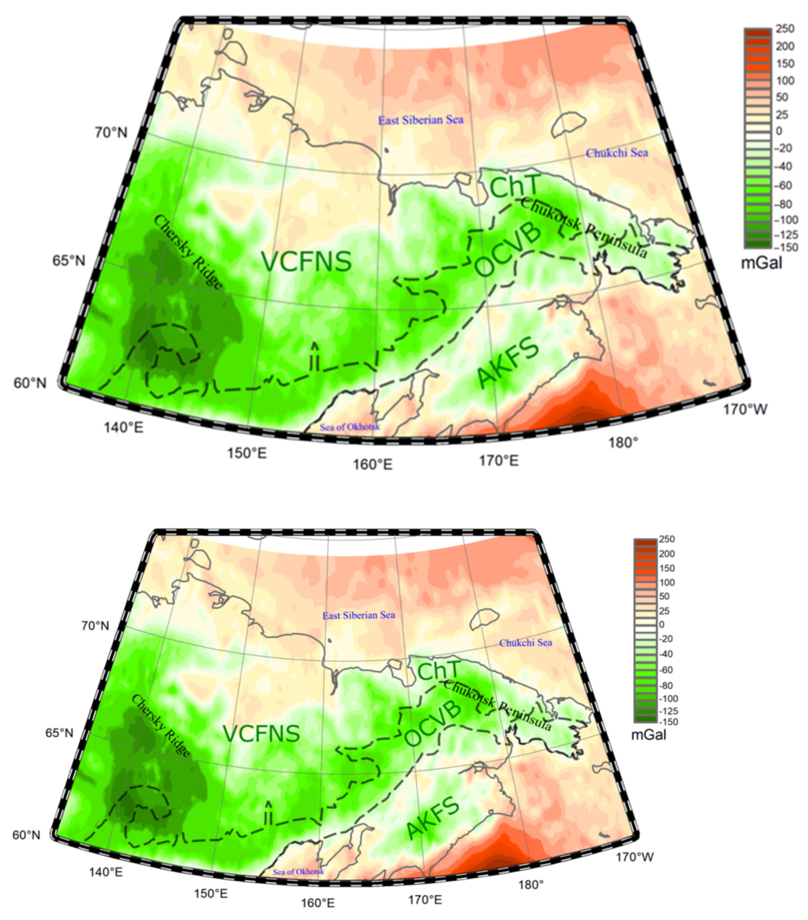
3.1.1. Bouguer Gravity Anomalies

The Bouguer gravity anomalies are based on the EIGEN-6c4 model [25]. This model was obtained as a combination of satellite data and ground observations. The maximal resolution is about 5ʹ × 5ʹ, which corresponds to the degree/order 2190 in spherical harmonics. The topography and bathymetry, which were used to compute the Bouguer gravity anomalies, are taken from the ETOPO-1 model [27]. It was assumed that the topography density is 2.67 g/cm³, and the water density is 1.03 g/cm³ (–1.64 g/cm³ relative to the accepted density of the topography). Their gravity effects were computed within a radius of 333.6 km (3 degrees), which was increased relative to the standard 222.4 km (2 degrees). Further, the increase of this radius would produce only very long wavelength anomalies, which are not considered here. The resulting Bouguer anomalies are shown in Figure 2. They represent the effect of all density anomalies beneath the Earth’s surface, excluding the effect of topography/bathymetry variations computed with the predefined constant density.

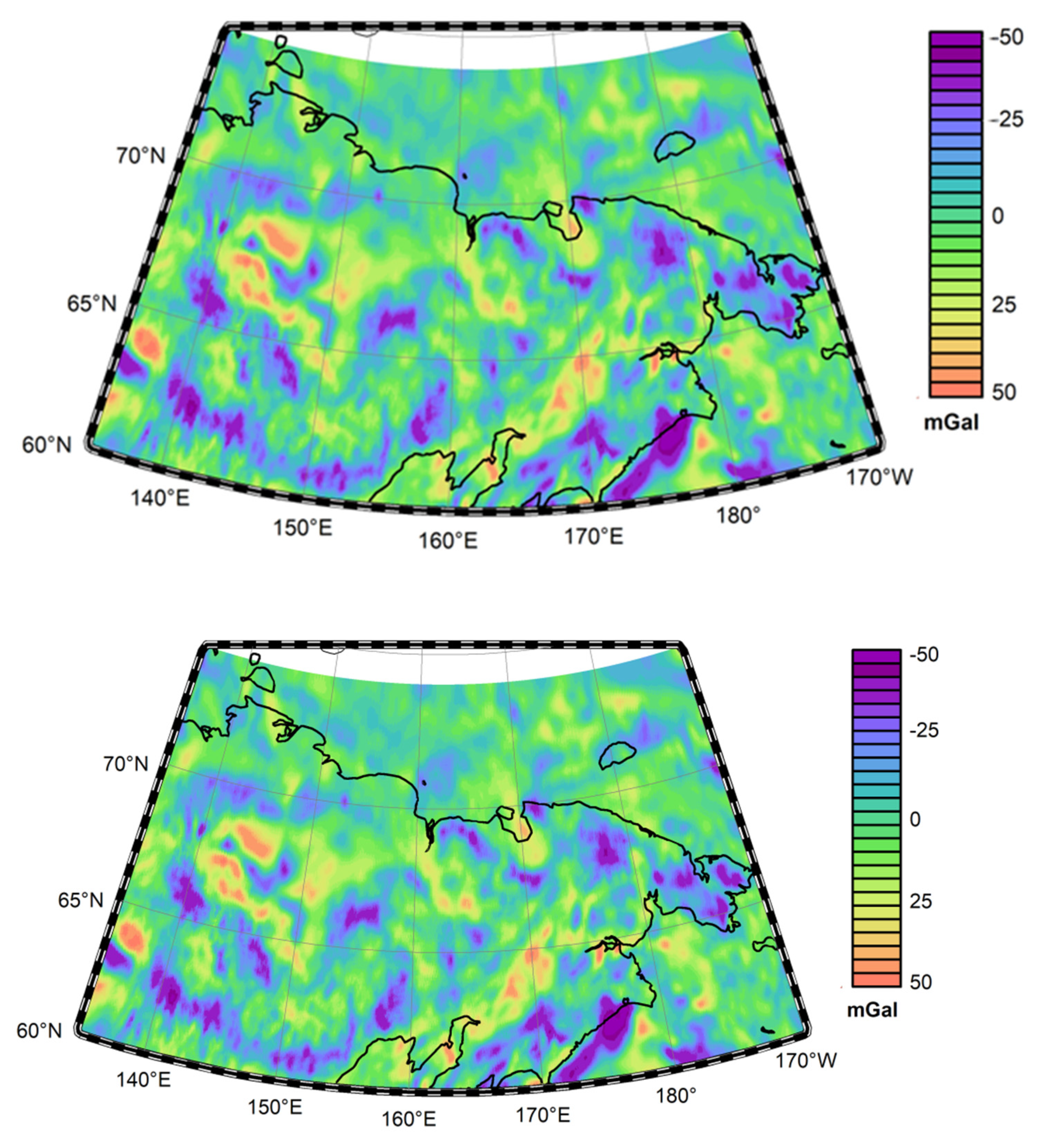
3.1.2. Isostatic Gravity Anomalies

The isostatic gravity anomalies are very similar to the mirrored topography because they are mainly induced by the masses compensated by the surface load (topography and bathymetry) in an isostatic sense [28]. The compensation is provided to a large extent by undulations of the Moho boundary. These deep anomalies significantly mask the effect of the crustal density heterogeneities, which are of great importance for geological interpretation. To eliminate the effect of these deep anomalies, isostatic correction is usually applied. In particular, this correction is important when we have limited data on the crustal structure. In this case, it is possible to assume that the topography and bathymetry are compensated according to a general compensation scheme. In spectral coordinates, the isostatic correction can be estimated following [29]:

$$∆g_{ic}\left(k_x,k_y\right)=-2\pi G\rho ·C·exp\left(-k·M\right)·t_{adj}\left(k_x,k_y\right),$$

(1)

where $k=\sqrt{k_x^2+k_y^2}$ is the wavenumber, k_x = 2π/λ_x and k_y = 2π/λ_y, M is the depth to the Moho and G is the gravitational constant. t_adj is the adjusted topography, which is estimated to match the bathymetry (t_b) and topography variations relative to the topography density ρ:

$$t_{adj}=t_b-\frac{{\rho }_w}{\rho }{t}_b,$$

(2)

where ρ_w = 1.03 g/cm³ is the water density. In the continental area, the second term in Equation (2) is not applied.

The parameter C determines the rate of the regional elastic compensation (C = 1 for the local compensation) and depends on the effective elastic thickness of the lithosphere (T_e) and wavenumber [30]:

$$C=∆\rho g/(k^{4}D+∆\rho g),$$

(3)

where $D=E{T}_e^3/\left[12\left(1-v^2\right)\right]$ is the flexural rigidity, v is the Poisson ratio, E is the Young modulus, ∆ρ is the average density difference between topography and the upper mantle, and g is the gravitational acceleration.

The isostatic gravity anomalies computed for the eastern part of the Russian Arctic zone [26] are shown in Figure 3. They can be considered as the main “geological” reduction of the observed gravity field [28].

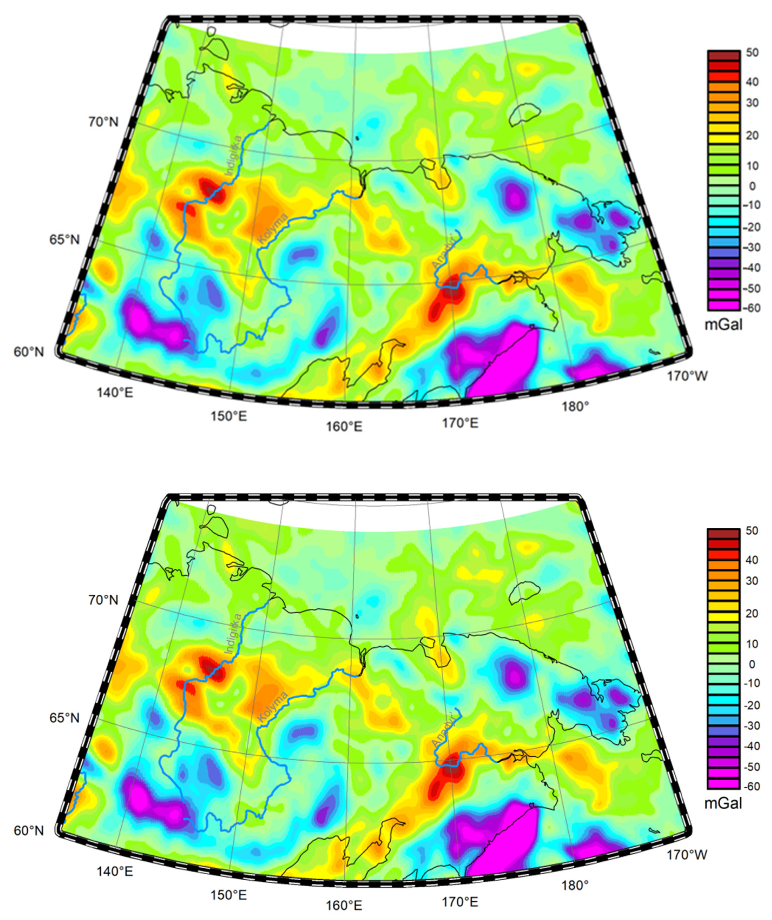
3.1.3. Decompensative Gravity Anomalies

The isostatic gravity anomalies can be successfully used for studying only relatively small (in a horizontal direction) structures of the crust. For large structures, their gravity effect can be again significantly reduced due to the isostatic compensation [31]. For the extended structures (300–400 km and more), this decrease can be even about one order of magnitude [32]. To eliminate this effect [31,33] suggested estimating the decompensative gravity correction.

This correction (Δg_dc) can be estimated following [34]:

$$∆g_{dc}\left(k_x,k_y\right)=\frac{1}{exp\left(k·M\right)/C-1}∆g_i\left(k_x,k_y\right),$$

(4)

where ∆g_i is the isostatic anomalies. This correction eliminates, to a large extent, the gravity field of compensation of the unknown density anomalies in the upper crust.

Unfortunately, the decompensative correction increases to infinity with increasing of the wavelength. The authors of [31] suggested introducing an upper limit for the size of the corrected anomaly. The maximum wavelength (λ₀ = 1500 km) is set following extended numerical tests [32,34]. A sum of the isostatic anomalies and the decompensative correction provides the decompensative gravity anomalies (Figure 4). This field chiefly shows density anomalies within the upper-mid crust. In particular, the negative anomalies largely represent the effect of sedimentary basins in the region, and many of them are still unknown [26].

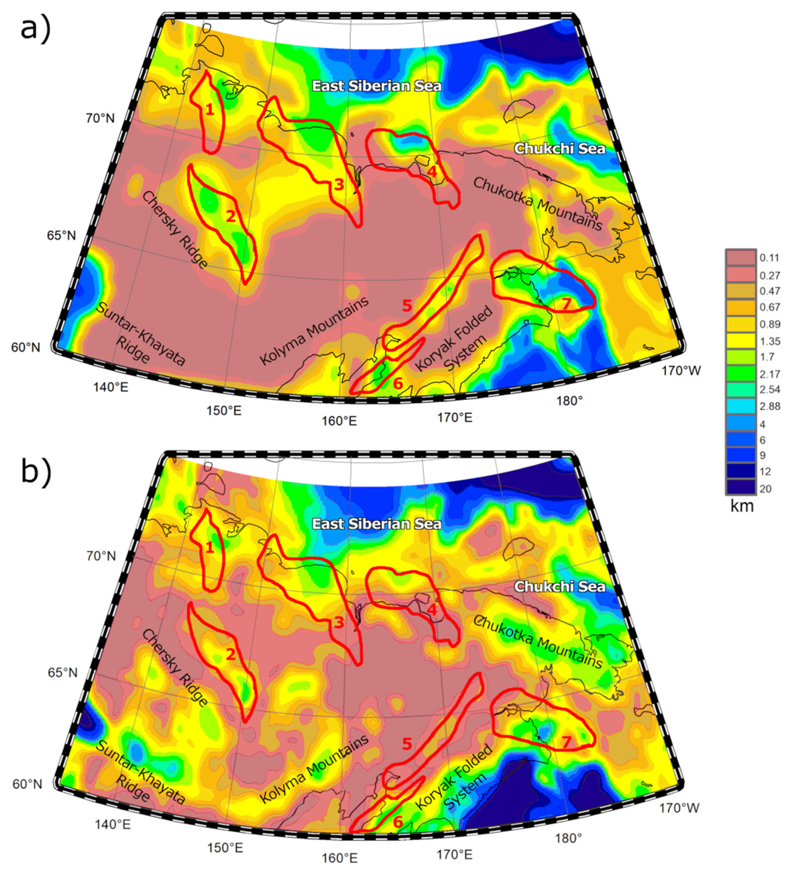
3.2. Structure of the Sedimentary Basins in the Eastern Part of the Russian Arctic Zone

The available data pertaining to the structural configuration and evolutionary history of several sedimentary basins in the Arctic region of Russia are currently inadequate, particularly with regard to the eastern segment. In contrast to the central and western regions, which host significant reserves of oil and gas [35], the subterranean structure of the sedimentary basins in the eastern region is largely unexplored. Consequently, the region has been designated for investigation using the recently developed decompensative gravity anomalies method [34]. The majority of sedimentary basins in this zone are identified by low thickness, which can be attributed to a relatively brief sedimentation period in the passive continental margins or intermontane depressions [36]. The most profound sedimentary basins in this vicinity are associated with grabens that extend to the Arctic shelf and were established on Late Mesozoic and Cenozoic foundations.

The approach based on decompensative gravity anomalies is described in Section 3.1. It was applied to the area from 135° to 190° E and 65° to 74° N (their locations are shown in Figure 5). The negative decompensative anomalies (Figure 4) were processed to determine the thickness of sediments, assuming appropriate density–depth relations for each basin [26]. This analysis revealed new features of the sedimentary basins related to their thickness and density, compared to the initial sedimentary cover model (Figure 5a), which included several sources [37,38,39] (only relatively deep basins with a sedimentary cover thickness of more than 0.5 km were analyzed). These sedimentary basins exhibit distinct phases of geological transformation, formed during various geological epochs (ranging from the Middle and Late Mesozoic to the Cenozoic) and in differing geological contexts. We present a concise overview of the geological structure of these basins; further elaboration can be found in [26].

The Primorsk basin is situated in the East Siberian lowland [36,40] and partly on the Arctic shelf (Figure 4). The sedimentary cover of this basin has been the subject of various studies and is found to vary significantly. West of the Primorsk basin lies the Tastakh basin, which, according to [41], is the marginal part of a larger depression, predominantly situated offshore. The sedimentary cover of the Tastakh basin comprises the Upper Mesozoic and Cenozoic (Paleogene–Neogene–Quaternary) strata. Another basin that is a part of the Arctic shelf is the Chauna Basin. It appeared in the Early Cretaceous [42] on the folded Early Mesozoic basement. Different ideas about the origin of this basin were formulated [36,40,43]. The sediments are represented by 2.2–2.5 km Upper Jurassic and Lower Cretaceous molasses and volcanogenic rocks [42].

The Penzhin Basin is situated within the Cenozoic fold belt segment, with its basement comprising Paleozoic and Mesozoic rocks. The sedimentary fill is composed of volcanic rocks ranging from Late Cretaceous to Cenozoic age. The Pustorets Basin is a depression situated on the west coast of northern Kamchatka, extending offshore. It measures 450 km in length and 50–100 km in width and rests on a Cretaceous folded basement. The sediments that fill the basin are of Cenozoic age. The uppermost part of the Cenozoic section comprises Oligocene–Miocene sediments, mostly consisting of sandstones and conglomerates with a thickness of up to 2.5 km. Finally, the Anadyr Basin, situated in the far eastern part of the study area, was created during the Late Mesozoic and Early Cenozoic periods, through the collision of the South Anyui Ocean in the convergence zones of different ages along the Asia continental margin and the Pacific Ocean plate. The basement of the basin was formed during the Late Cretaceous (Albian–Cenomanian) orogeny. The sedimentary cover’s evolutionary history can be divided into three phases:

(1)

Accumulation of sediments during the passive continental margin phase (Late Cretaceous–Early Eocene);

(2)

Accumulation of sediments during the Middle Eocene–Oligocene period due to extension and compression in the basin’s southern part caused by the Koryak accretion orogeny;

(3)

Accumulation of Miocene sediments during continental rifting conditions [44].

The new geological and tectonic features revealed by the decompensative gravity anomalies approach are presented in detail in [26]; they imply the changes and redistributions of the sedimentary thickness for the analyzed basins. The sedimentary cover model obtained using this approach is shown in Figure 5b. In this paper, we list some principal changes in the sedimentary thickness and density:

• For the Anadyr basin in its continental part, the thickness is reduced to 1–2 km compared to previous surveys. Although the thickness is higher in some very local depressions [44], which are not resolved by the new model, the northward decrease trend is visible for the continental part in both models, indicating that the new modeling approach provides sufficiently reliable results, at least qualitatively.
• In the central part of the Penzhin basin, the thickness appears to be lower by about two times compared to the initial model.
• For the Pustorets basin, the new location of the depocenter is identified.
• For the Primorsk basin, the new model also shows a significant reduction of the sedimentary cover in the southeast direction.
• In the offshore part of the Chauna basin, the sedimentary thickness appears to be 2–2.5 km according to the new model, which is lower than in the initial model (4 km); however, the new result agrees with the marine seismic surveys, which confirms the robustness of the method.
• In the northern part of the Zyryanka basin, the connection of two coal-bearing zones, revealing the features of the Lower Cretaceous strata not previously mapped due to insufficient geological surveys, is identified by the new model.

The mentioned basins are still poorly studied, so a direct comparison for the validation of the results is still impossible. Nevertheless, the sedimentary cover model generally matches the geological structure of the basins according to the most consistent results listed in [26]. Therefore, the sedimentary cover models obtained from that study were included in the dataset for the Arctic lithosphere.

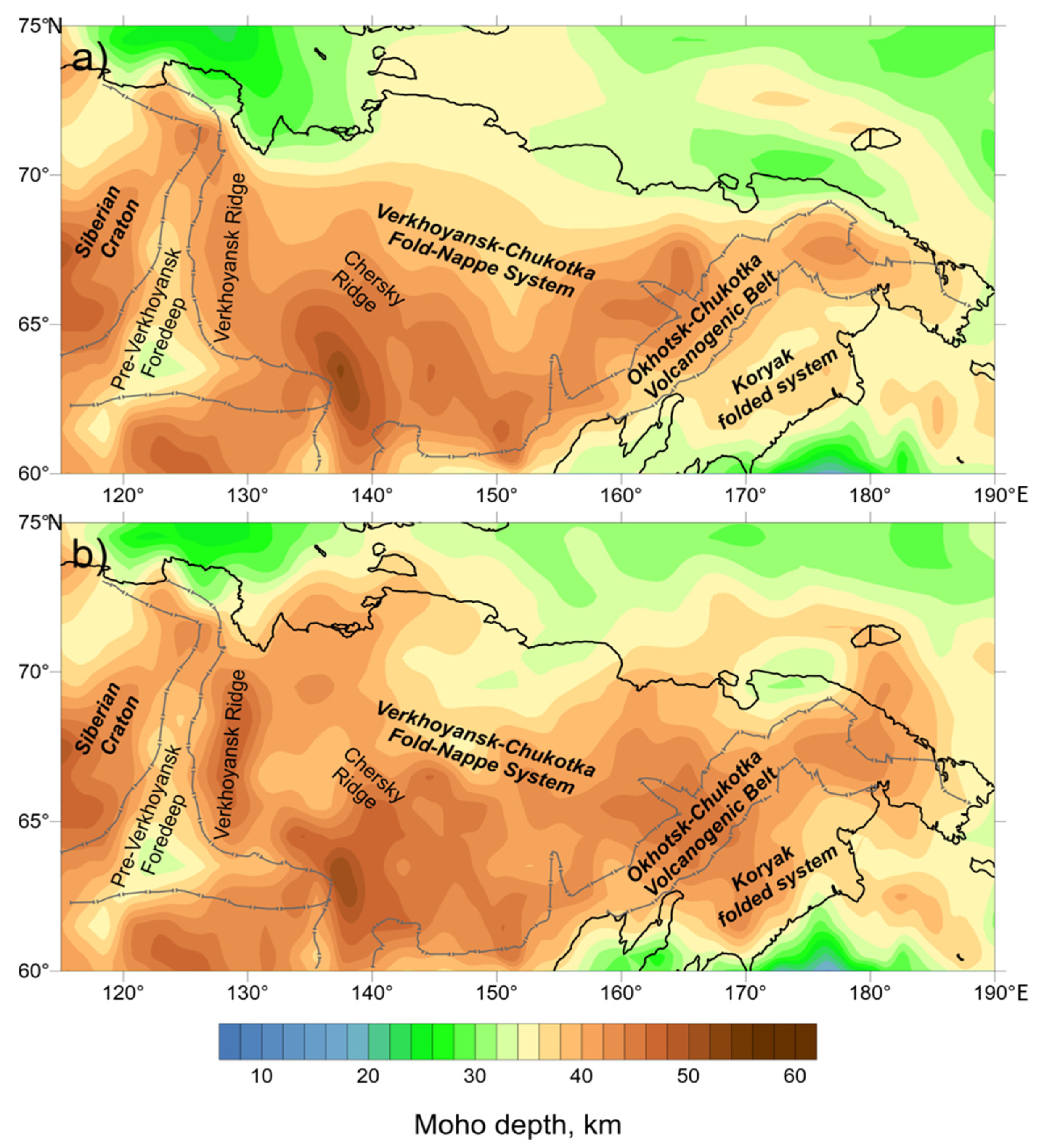
3.3. Depth to the Moho in the Eastern Part of the Russian Arctic Zone

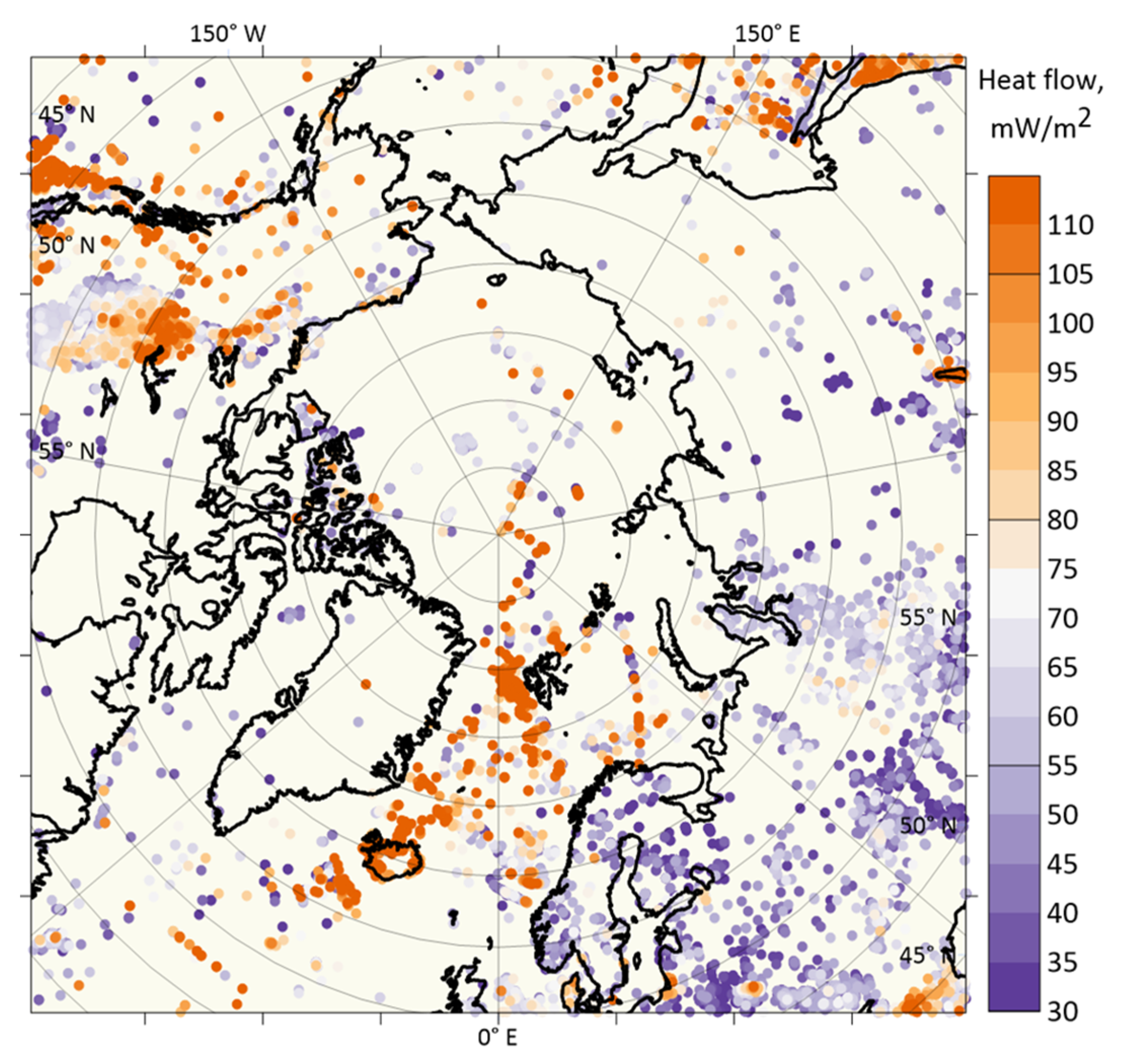
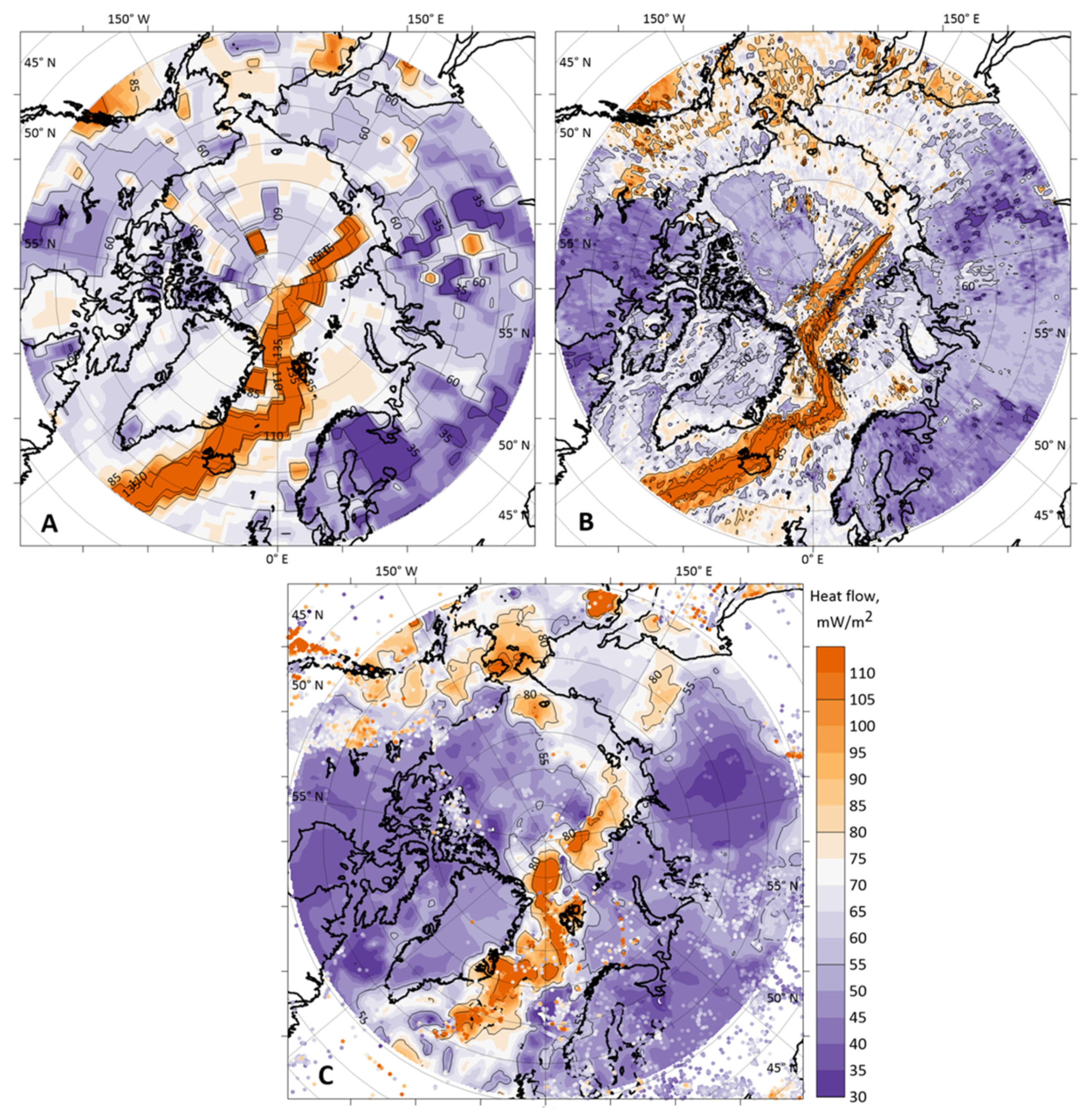
The Moho discontinuity is one of the most important boundaries within the Earth, and it is characterized by strong changes in all physical parameters [45]. Therefore, knowledge of the Moho depths is extremely important for any kind of geophysical modeling and for understanding the lithosphere structure and dynamics, and this was the reason to include the Moho depth data in the dataset on the Russian Arctic lithosphere. Direct data on the Moho depth can be only obtained from seismic studies, for which coverage is extremely heterogeneous. In particular, seismic determinations are almost not available in the eastern part of the Russian Arctic zone, which is an extremely hard-to-access area [13]. The new Moho map has been obtained for this region (60–75° N, 110–190° E) [18]. This area is unique in its structure, as it includes several tectonic elements of different ages — from Paleozoic to Early Cenozoic [46,47]. The Moho map is based on a joint inversion of various geophysical fields, primarily the residual gravity field and vertical gravity gradients. The initial map of [13] was corrected to fit these fields with additional constraints from several seismic profiles carried out in 1989–2012 during several research projects and collected by VSEGEI and VNIIOkeangeologia [13].

The Moho depth model (Figure 6b) was compared in detail with the initial model of [13] (Figure 6a).

This model essentially improved the existing Moho maps for the Russian Arctic zone and the model [13], and, in particular, displays some features which were absent in the previous models. First, it reveals the crustal root with a depth of 47 km under the Verkhoyansk Ridge, compared to a relatively shallow depression of the Moho in the initial model. Such crustal thickening is typical for mountain ridges, which confirms that the resulting model is robust. Next, a significant change in the Moho depth (from 25–40 to 38–45 km) is obtained in the northern continental part of the study area and offshore. We hypothesize that this thickening of the crust is related to underplating due to the former plume activity. The offshore part of the Chukotka microcontinent is characterized by a crustal thickness of 38–42 km in the Verkhoyansk–Chukotka fold belt margin and 42–44 km under the Chukotka Peninsula. The zone of relatively thin (26–28 km) crust underlying the Chukchi Sea appears to be less extended as compared to the initial model. On the other hand, the Moho depth maximum (42 km) under the OCVB has not been modified in the obtained model. Finally, the crustal thickness under the Anadyr–Koryak folded system location has been increased by up to 10 km. This matches the general ideas of the development of this folded system [48,49]. The Moho model was compared with the ArcCrust model based on a 3D gravity inversion constrained by other geophysical data. The ArcCrust model provides much fewer details compared to our map in the continental part, in particular, for the maximum associated with the northern part of the Verkhoyansk Ridge. In general, the ArcCrust model gives more thick crust for the northern part of the study area, which is probably due to the insufficient resolution of the initial data.

3.4. Heat Flow Map

The study of heat flow is an important part of geophysical research and provides additional data on the tectonics and internal structure of the Earth’s crust and lithosphere. Data on the thermal structure of the lithosphere are especially important at high latitudes covered by permafrost. In particular, considering climate change trends, it is important to know the heat flow for calculating the long-term stability of engineering structures and estimating potential greenhouse gas emissions resulting from permafrost thawing. Heat flow data are also necessary for estimating potential geothermal energy reserves. However, data obtained from direct measurements are insufficient to produce a detailed heat flow map for most of the Arctic region, especially for the remote and poorly studied areas of northeastern Eurasia.

To build a heat flow map for the study region, we used the catalog prepared by the International Heat Flow Commission (IHFC, www.ihfc-iugg.org, accessed on 11 March 2023) as an initial approximation (Figure 7). The most recent version of this global database covers the measurement period from 1939 to 2021 and contains n = 74,548 records from 1403 publications. A total of 55% of the heat flux values presented are in the continental region (n~40,870), while the remaining 45% are in the oceanic region (n~33,678). The polar zone above the sixtieth latitude has about 2920 records of varying quality.

However, this database contains large gaps, especially in the northeastern part of the Eurasian continent. To fill these gaps, we used theoretical models for global heat flux [51,52], which are based on interpolating measured data to account for the structure of the lithosphere (Figure 8A,B). Then, a method was developed for estimating the surface heat flux using inversion of seismic and magnetic data, supported by direct measurements [21]. This approach allows for using all available indirect data on the thermal structure of the lithosphere to build a thermal model by the optimization method and minimize errors arising from the uncertainty of input data. The resulting heat flow map (Figure 8C) agrees well with the observational data and correlates with lithospheric domains of different tectonic history and age correspondingly. The heat flow map is an essential part of the presented dataset, as the map reveals some features that were not identified earlier (compare Figure 8A–C). In particular, it displays the zones of increased heat flow in the Bering Strait and Chukchi Sea, and a residual anomaly in the area of the Mid-Labrador Ridge, which was active in the Paleogene. The geothermal data also clearly show an increase in heat flow in the ancient rift zone separating Eastern and Central Siberia, which was not visible on maps published earlier (Figure 8A,B).

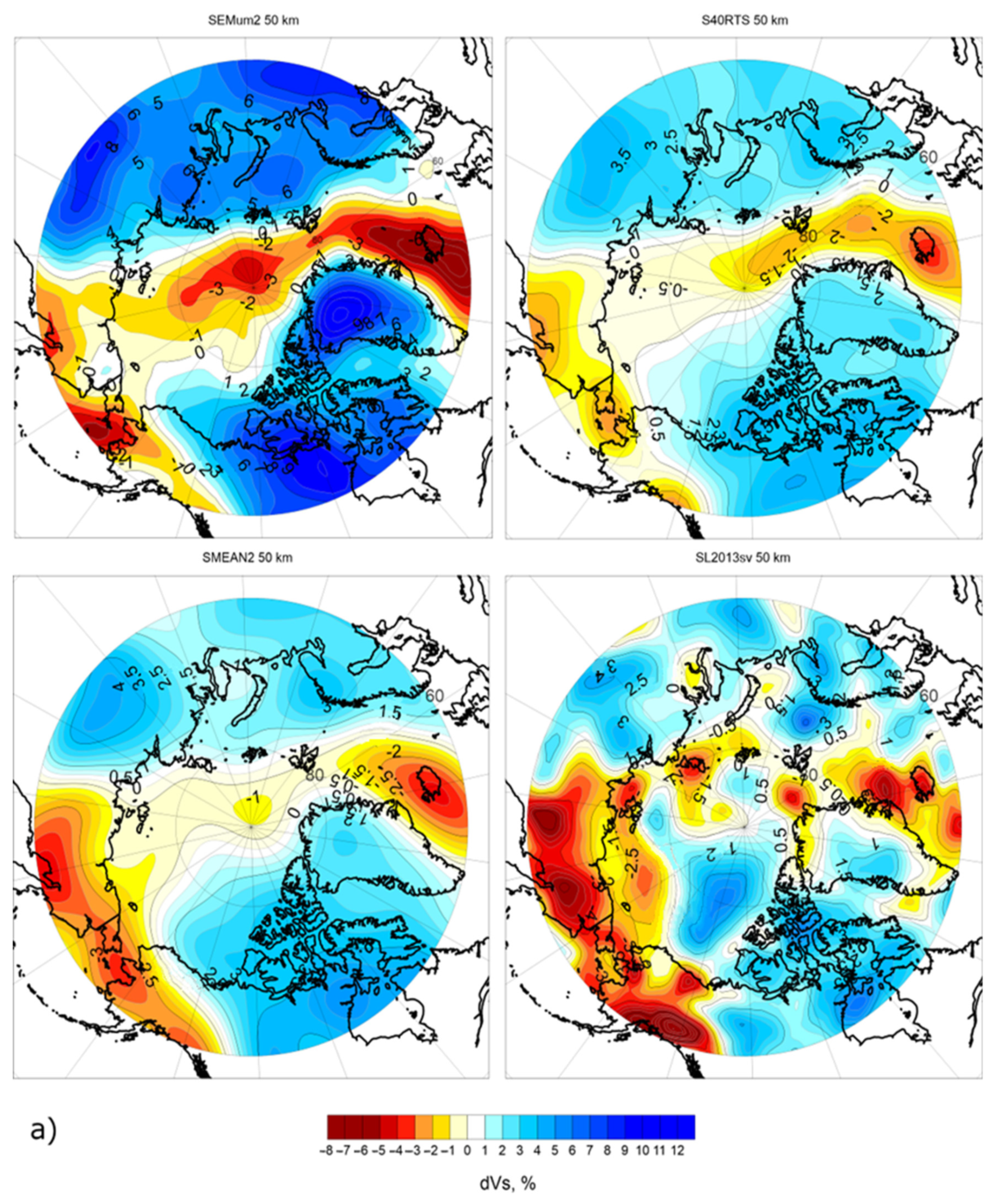
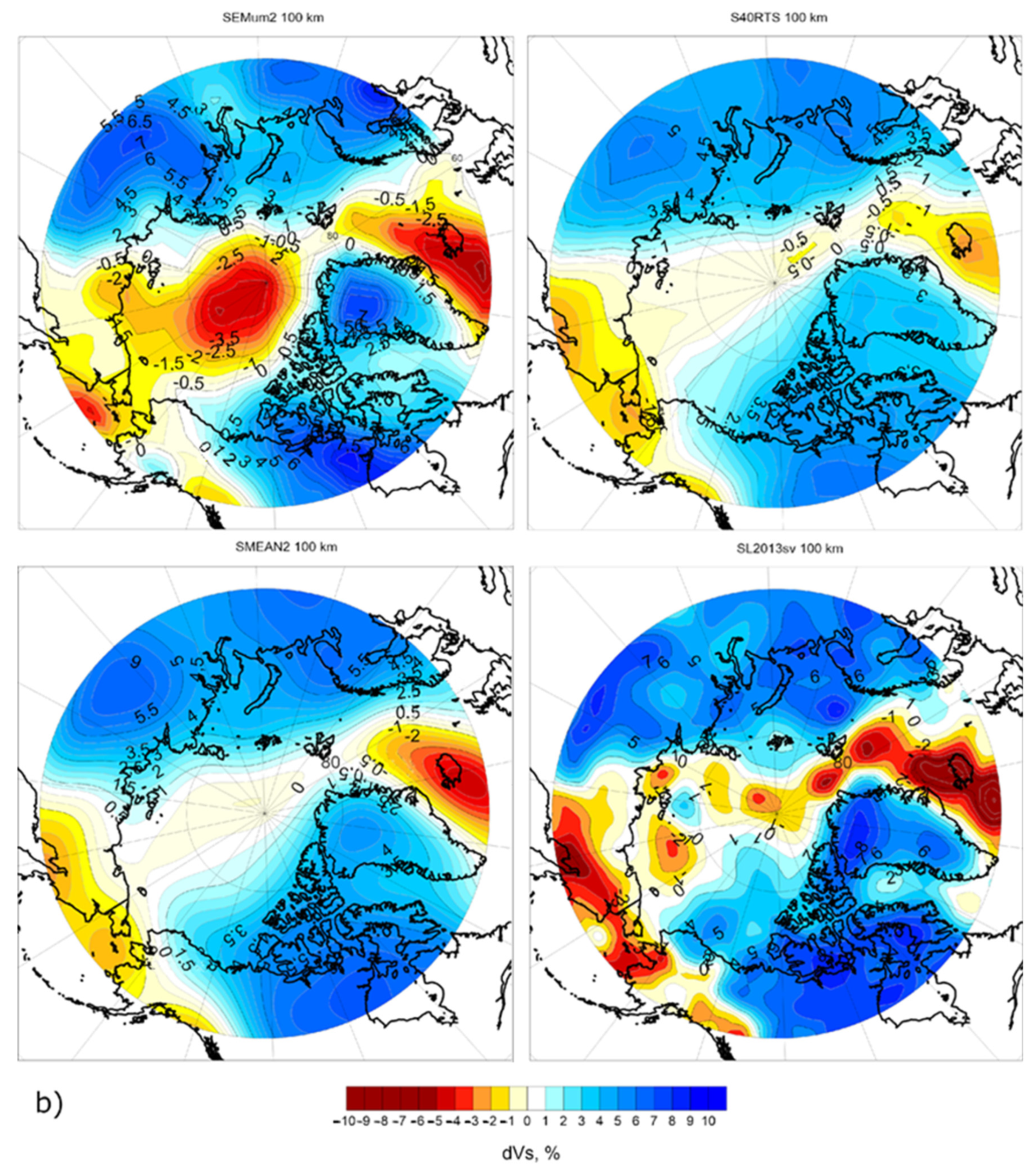
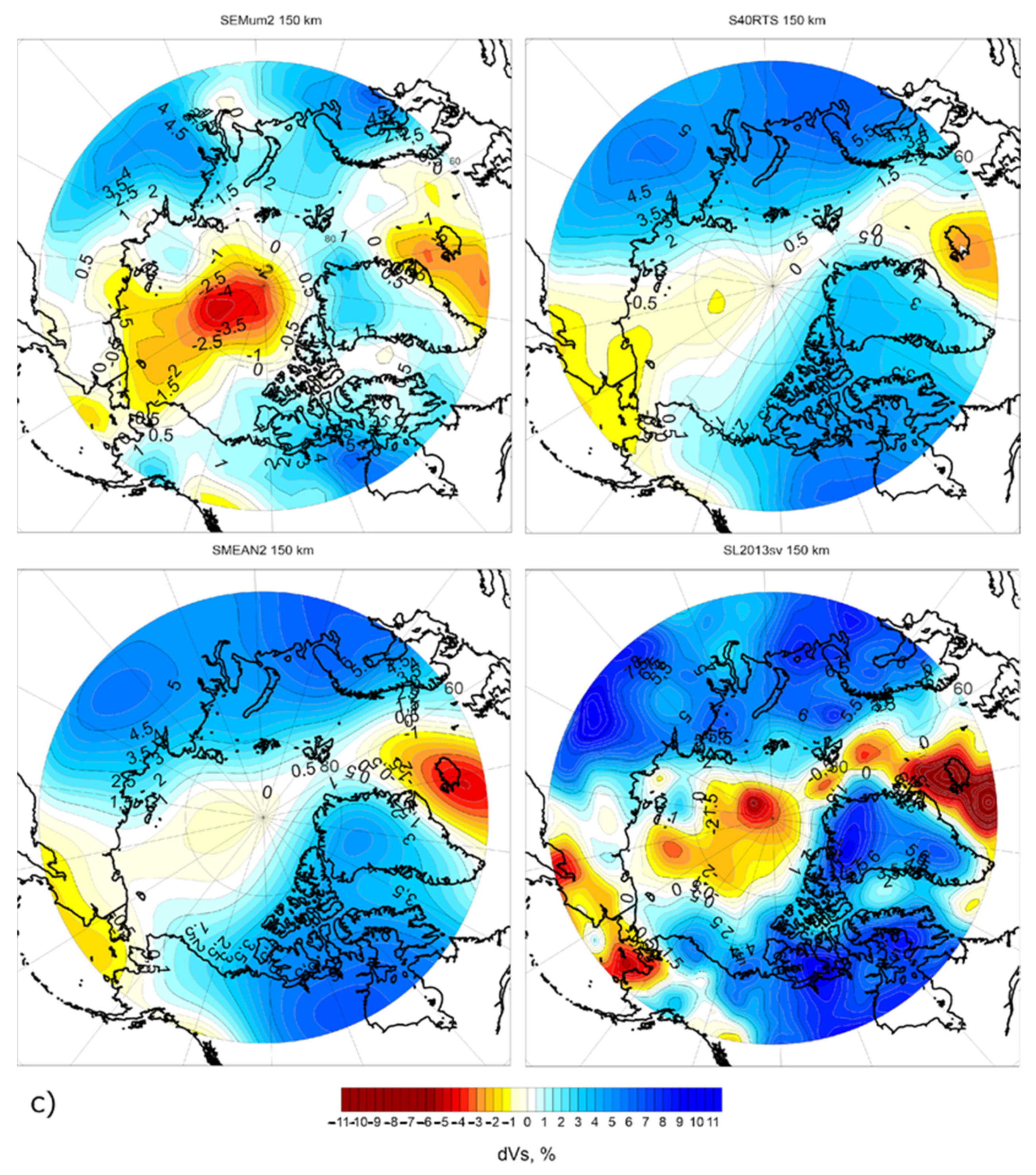
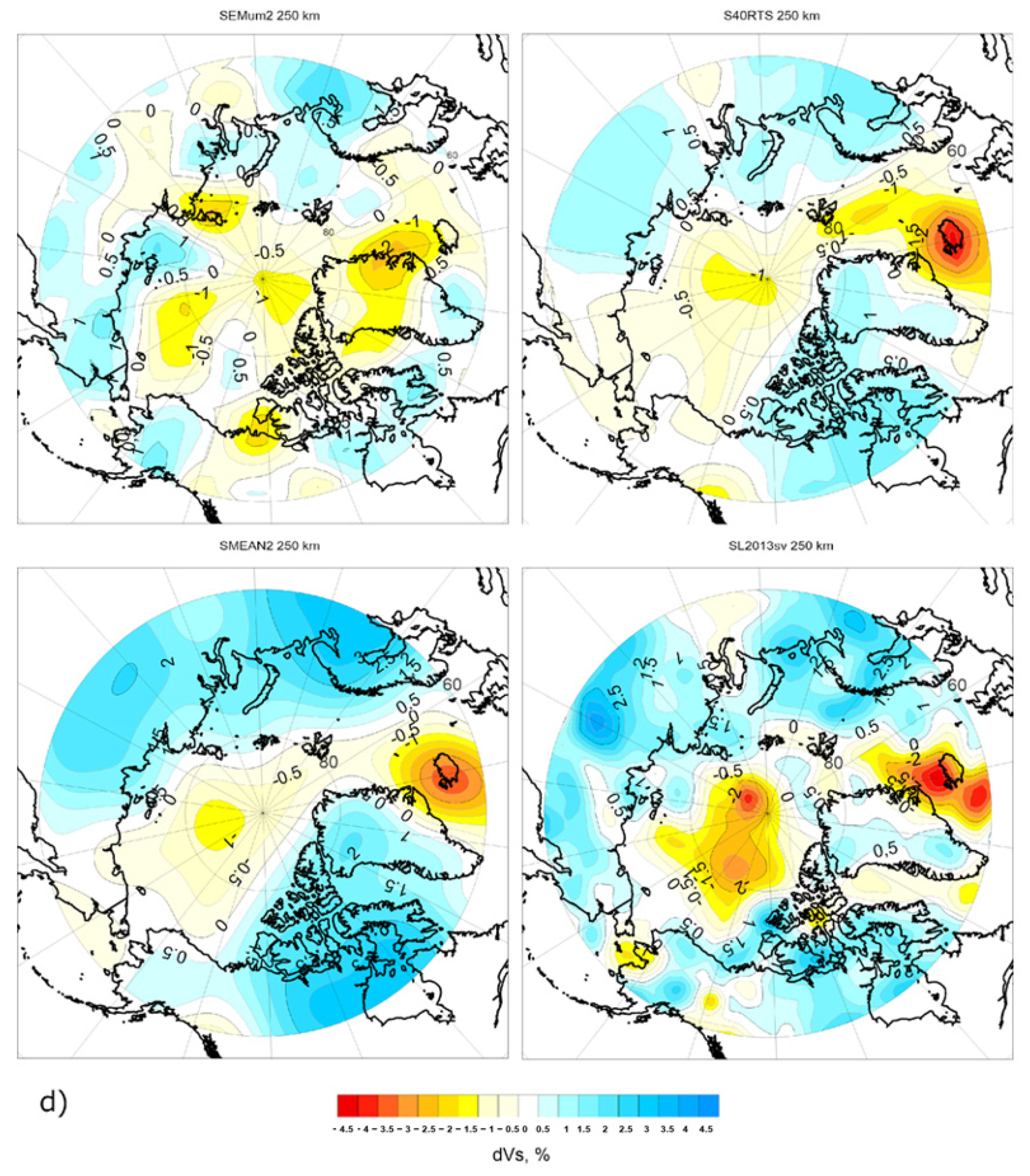
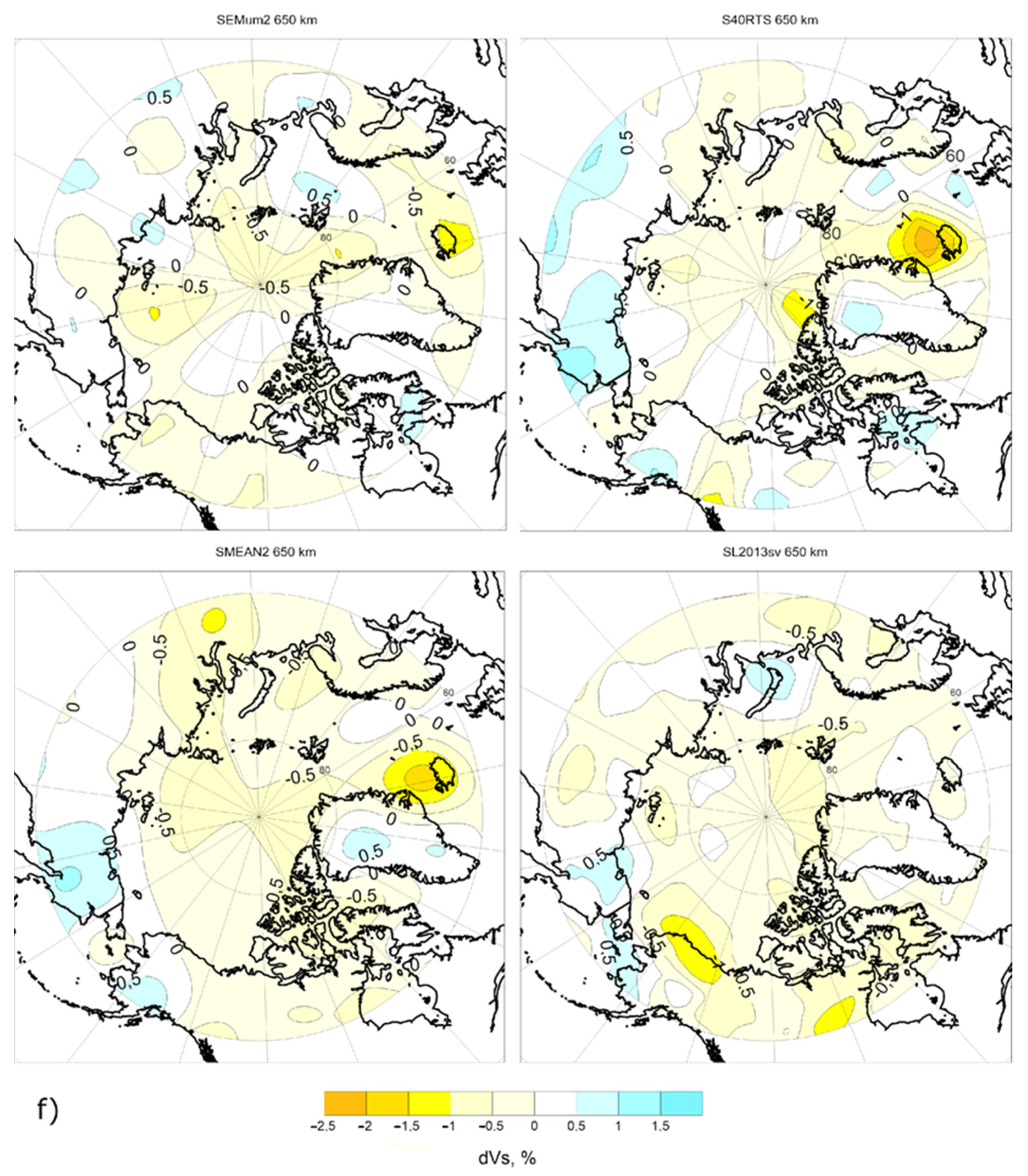
3.5. Seismic Tomography

In combination with other geophysical methods, seismic tomography is one of the most important sources on the structure of the Earth’s lithosphere and mantle. To detect crustal, lithospheric, core, and mantle heterogeneity, various seismic tomography techniques have been developed, depending on data availability and seismic wave types. Methods based on the inversion of the body waves generally show better resolution in areas with sufficiently dense ray paths connecting earthquakes and seismic stations [53]. The Arctic region is characterized by a relatively sparse density of wave paths due to the uneven distribution of the sources (earthquakes) located mainly along the Pacific subduction zone and an insufficient number of seismic stations in this region. Furthermore, the global P-wave tomography models are usually aimed at studying the structure of the deep mantle and core, which are not the topics of this study. Surface waves are more applicable for studying the crust and uppermost mantle [54]. In global models, they are often applied in combination with S or P body waves. Since the Earth’s surface is unevenly covered by seismic wave sources and receivers, methods based on shear (S)-wave inversion (chiefly based on the surface waves) are most applicable for the tomographic models of the lithosphere and upper mantle. Below, we consider the Circumpolar Arctic segments taken from several existing global S-wave tomography models.

For the investigation of the Russian Arctic zone, the SL2013sv tomography model [54], based on a joint inversion of the surface and shear waves, was chosen as the basic one. This model has the best resolution to depths of 300–350 km, therefore covering the whole lithosphere. For a comparative analysis, we also analyze the alternative models: SEMum2 [55], S40RTS [56], and a composite model SMEAN2 compiled from S40RTS, GyPSuM [54], and SAVANI [57,58]. For comparison of the alternative models, we built the depth slices of the S-wave velocity anomalies (dV = dV_S/V_S, in %) for SL2013sv for three alternative models for the depths from 50 to 700 km down with a step of 50 km.

In Figure 9, the depth slices of SEMum2, S40RTS, and SMEAN2 models are compared with the SL2013sv model at 50, 100, 150, 250, 400, and 650 km (to the upper mantle bottom). At first glance, the SEMum2 and S40RTS data display similar features in velocity anomalies for the continental and oceanic lithosphere depending on the thickness and age. The areas of the ancient cratons, such as North America or Siberia, are characterized by positive dV values, whereas in the areas of the Arctic Ocean, North Eastern Asia, and Alaska, the anomalies are mainly negative. However, two intense velocity anomalies related to the deep structure of the Siberian and East European cratons are visible in the SEMum2 model for Eurasia, whereas the corresponding anomalies in the S40RTS model are about two times less. The SEMum2 model also displays more high-frequency details for the North American craton (especially for Greenland). Although the SL2013sv model generally repeats the basic features observed in the SEMum2 and S40RTS models, it demonstrates many more small-scale details similar to SEMum2 for Siberia, Greenland, and the Arctic Ocean basins.

At the 100 and 250 km depths (Figure 9b,c), SL2013sv again demonstrates much higher resolution compared to the other three models. Within several hundred kilometers from the surface, the main velocity anomaly contours and even individual features of the SMEAN2 model depth slices are largely similar to the S40RTS slices at the same depths because SMEAN2, which is a compilation of several models, is chiefly contributed to by S40RTS at these depths. In contrast, the SEMum2 slices for these depths again display some clear and well-contoured details of the velocity distribution. The negative velocity anomaly (−0.5 … −1%) visible in Northern Eurasia in the SEMum2 slice can be related to the corresponding LAB rise from 200 to 60–80 km in this location, according to the lithosphere–asthenosphere LAB data from the LITHO1 model [59].

At the depths of 400–650 km (Figure 9e,f), the differences between all four models become less noticeable due to the decrease of the amplitudes to 0.5–1%. At these depths, it becomes hard to identify specific features of the velocity distribution. The major difference between the SL2013sv and the other three models at these depths is the strong negative velocity anomaly related to the Iceland plume. It is observed at 50 km for S40RTS and SMEAN2, remains at all their slices, not changing its location significantly, and decays with depth in the SL2013sv model, as well as in SEMum2.

The comparison of the abovementioned seismic tomography models shows that the SL2013sv model has the best resolution in the upper mantle. All three alternative tomography models display the large-scale details of the lithosphere structure and LAB similarly and, for particular depths, they are close to SL2013sv but without small-scale details revealed by the latter. In the upper segment of the upper mantle (0–400 km approximately), SEMum2 also demonstrates better spatial resolution than the S40RTS and SMEAN2 models. It also better agrees with the LAB depths (LITHO1). Therefore, the SEMum2 model is considered the best alternative model for further use in the investigation of the Russian Arctic zone.

4. Conclusions

In this work, we prepared an integrated database that contains geological and geophysical information for the Arctic zone of Russia and some surrounding area. This is a compilation of the models obtained as a result of original research (isostatic and decompensative gravity anomalies, sedimentary cover models, the Moho depth map, and the geothermal heat flow map) and the data derived from freely available resources (e.g., the depth slices from four seismic tomography models). The dataset comprises the gravity field and its reductions, sedimentary cover, Moho models, the geothermal heat flow map, and, finally, the seismic tomography slices for the lithosphere and the upper mantle. Therefore, it allows studying not only the geological structures and development of various zones of the lithosphere but also the dynamics of processes occurring at depths up to 650 km. The paper provides examples of several previously known models with clarification of the most reliable ones for the study area, as well as the physical fields and main crustal boundaries calculated by the authors, which refine the characteristics of the region. An integrative analysis of the parameters provided by the database will make it possible to evaluate the deep geological structures, as well as to understand near-surface processes such as permafrost melting.

The analysis of the gravity field given in the paper allows the calculation of several reductions, which are more appropriate for geological purposes. In addition to the conventional Bouguer anomalies, we calculate the isostatic and decompensative anomalies of the gravity field. The isostatic anomalies are largely refined from the deep effects and, therefore, are better for studying the near-surface structures. Furthermore, the decompensative anomalies are calculated to separate the unbiased effect of near-surface structures such as large sedimentary basins. Their analysis further makes it possible to refine the model of the sedimentary cover, including the thickness and density, for the least studied areas with complicated geological structures, such as the Tastakh, Zyryanka, Primorsk, Chauna, Penzhin, Pustorets, and Anadyr basins. For correction of the existing Moho depth model, we used the gravity field gradients in addition to the gravity field. By this, we significantly reduced the number of possible solutions, which is typical for gravity field analysis. The previous models are based on existing seismic determinations, which are almost absent in the study area. Therefore, these models contain large smooth gradient zones resulting from the distant extrapolation. The present work provides the refined depths that differ from the starting model by several kilometers for such regions as the Verkhoyansk–Chukotka fold–nappe system, Kolyma–Omolon composite superterrane, Laptev rift system, South Anyui suture zone, Okhotsk–Chukotka volcanogenic belt, and Anadyr–Koryak folded system.

A surface heat flow map included in the dataset is based on a joint inversion of multiple geophysical data constrained by the observations from the International Heat Flow Commission catalog. It provides many more details, especially for the areas with few or without observations, such as the Bering Strait, Chukchi Sea, and the Mid-Labrador Ridge; moreover, it reveals the position of the rift zone separating the Eurasian Plate from the North American plate.

We also evaluated several tomographic models to determine the most relevant for studies of the deep interiors. A comparison of the SEMum2, S40RTS, SMEAN2, and SL2013sv models was carried out, with an assessment of the reliability and horizontal resolution of the seismic velocities and main lithospheric boundaries in the study area. We conclude that the SL2013sv model better describes the structure of the upper mantle.

In conclusion, this work presents and visualizes a large amount of data, which will allow for a detailed geological and geophysical interpretation, as well as make it possible to build various 3D models of the region. All the data are publicly available and can be downloaded from the specified repository at the World Data Center for Solid Earth Physics website: http://www.wdcb.ru/arctic_antarctic/arctic_geoph.fields.html (accessed on 14 April 2023).

References

1. Bortnikov, N.S.; Lobanov, K.V.; Volkov, A.V.; Galyamov, A.L.; Vikentev, I.V.; Tarasov, N.N.; Distlerov, V.V.; Lalomov, A.V.; Aristov, V.V.; Myrashkov, K.Y.; et al. Strategic metal deposits of the Arctic Zone. Geol. Ore Depos. 2015, 57, 433–453. (In Russian) [Google Scholar] [CrossRef]
2. Kulikov, V.A. Geophysics of Solid Minerals; PoliPRESS LLC: Moscow, Russia, 2017; p. 208. ISBN 978-5-9500750-2-5. (In Russian) [Google Scholar]
3. Lalomov, A.V.; Bochneva, A.A. Rare-metal potential of placer deposits and weathering crusts of the Russian Arctic. Arct. Ecol. Econ. 2018, 4, 111–122. (In Russian) [Google Scholar] [CrossRef]
4. Chanysheva, A.; Ilinova, A. The Future of Russian Arctic Oil and Gas Projects: Problems of Assessing the Prospects. J. Mar. Sci. 2021, 9, 528. [Google Scholar] [CrossRef]
5. Dziadek, R.; Ferraccioli, F.; Gohl, K. High geothermal heat flow beneath Thwaites Glacier in West Antarctica inferred from aeromagnetic data. Commun. Earth Environ. 2021, 2, 162. [Google Scholar] [CrossRef]
6. Makarieva, O.M.; Nesterova, N.V.; Beldiman, I.N.; Lebedeva, L.S. Actual Problems of Hydrological Assessments in the Arctic Zone of Russian Federation and Adjacent Permafrost Territories. Arct. Antarct. Res. 2018, 64, 101–118. (In Russian) [Google Scholar] [CrossRef]
7. Petrunin, A.G.; Rogozhina, I.; Vaughan, A.P.M.; Kukkonen, I.T.; Kaban, M.K.; Koulakov, I.; Thomas, M. Heat flux variations beneath central Greenland’s ice due to anomalously thin lithosphere. Nat. Geosci. 2013, 6, 746–750. [Google Scholar] [CrossRef]
8. Rogozhina, I.; Petrunin, A.G.; Vaughan, A.P.M.; Steinberger, B.; Johnson, J.V.; Kaban, M.K.; Calov, R.; Rickers, F.; Thomas, M.; Koulakov, I. Melting at the base of the Greenland ice sheet explained by Iceland hotspot history. Nat. Geosci. 2016, 9, 366–369. [Google Scholar] [CrossRef]
9. Rogozhin, E.A.; Kapustian, N.K.; Antonovskaya, G.N.; Konechnaya, Y.V. New seismicity map for the European sector of the Russian Arctic region. Geotectonics 2016, 50, 238–243. [Google Scholar] [CrossRef]
10. Kozyreva, O.V.; Pilipenko, V.A.; Marshalko, E.E.; Sokolova, E.Y.; Dobrovolsky, M.N. Monitoring of Geomagnetic and Telluric Field Disturbances in the Russian Arctic. Appl. Sci. 2022, 12, 3755. [Google Scholar] [CrossRef]
11. Gvishiani, A.D.; Vorobieva, I.A.; Shebalin, P.N.; Dzeboev, B.A.; Dzeranov, B.V.; Skorkina, A.A. Integrated Earthquake Catalog of the Eastern Sector of the Russian Arctic. Appl. Sci. 2022, 12, 5010. [Google Scholar] [CrossRef]
12. Drachev, S.S. Fold belts and sedimentary basins of the Eurasian Arctic. Arktos 2016, 2, 21. [Google Scholar] [CrossRef]
13. Petrov, O.; Morozov, A.; Shokalsky, S.; Kashubin, S.; Artemieva, I.M.; Sobolev, N.; Petrov, E.; Ernst, R.E.; Sergeev, S.; Smelror, M. Crustal structure and tectonic model of the Arctic region. Earth-Sci. Rev. 2016, 154, 29–71. [Google Scholar] [CrossRef]
14. Rekant, P.V.; Gusev, E.A. Sediments in the Gakkel Ridge rift zone (Arctic Ocean): Structure and history. Russ. Geol. Geophys. 2016, 57, 1283–1287. [Google Scholar] [CrossRef]
15. Kanao, R.; Suvorov, V.; Toda, S.; Tsuboi, S. Seismicity, structure and tectonics in the Arctic region. Geosci. Front. 2015, 6, 665–677. [Google Scholar] [CrossRef]
16. Kashubin, S.N.; Petrov, O.V.; Androsov, E.A.; Morozov, A.F.; Kaminsky, V.D.; Poselov, V.A. Crustal types in the Circumpolar Arctic. Reg. Geol. Metallog. 2013, 55, 5–20. (In Russian) [Google Scholar]
17. Filatova, N.I.; Khain, V.E. Development of the Verkhoyansk–Kolyma orogenic system as a result of interaction of adjacent continental and oceanic plates. Geotectonics 2008, 42, 258–285. [Google Scholar] [CrossRef]
18. Kaban, M.K.; Sidorov, R.V.; Soloview, A.A.; Gvishiani, A.D.; Petrunin, A.G.; Petrov, O.V.; Kashubin, S.N.; Androsov, E.A.; Milshtein, E.D. A New Moho Map for North-Eastern Eurasia Based on the Analysis of Various Geophysical Data. Pure Appl. Geophys. 2022, 179, 3903–3916. [Google Scholar] [CrossRef]
19. Lebedev, S.; Schaeffer, A.J.; Fullea, J.; Pease, V. Seismic tomography of the Arctic region: Inferences for the thermal structure and evolution of the lithosphere. Geol. Soc. Lond. Spec. Publ. 2018, 460, 419–440. [Google Scholar] [CrossRef]
20. Tesauro, M.; Kaban, M.K.; Aitken, A.R.A. Thermal and compositional anomalies of the Australian upper mantle from seismic and gravity data. Geochem. Geophys. Geosyst. 2020, 21, e2020GC009305. [Google Scholar] [CrossRef]
21. Petrunin, A.G.; Soloviev, A.A.; Sidorov, R.V.; Gvishiani, A.D. Inverse-forward method for heat flow estimation, a case study for the Arctic region. RJES 2022, 22, ES6004. [Google Scholar] [CrossRef]
22. Hager, B.H.; O’Connel, R.J. A simple global model of plate dynamics and mantle convection. J. Geophys. Res. Solid Earth 1981, 86, 4843–4867. [Google Scholar] [CrossRef]
23. Kaban, M.K.; El Khrepy, S.; Al-Arifi, N. Density structure and isostasy of the lithosphere in Egypt and their relation to seismicity. Solid Earth 2018, 9, 833–846. [Google Scholar] [CrossRef]
24. Kaban, M.K. Gravity Anomalies, Interpretation; Encyclopedia of Earth Sciences Series; Springer: Cham, Switzerland, 2019; pp. 1–7. [Google Scholar] [CrossRef]
25. Förste, C.; Abrykosov, O.; Lemoine, J.-M.; Flechter, F.; Balmino, G.; Barthemes, F. EIGEN-6C4 The latest combined global gravity field model including GOCE data up to degree and order 2190 of GFZ Potsdam and GRGS Toulouse. GFZ Data Serv. Potsdam Ger. 2014. [Google Scholar] [CrossRef]
26. Sidorov, R.V.; Kaban, M.K.; Soloviev, A.A.; Petrunin, A.G.; Gvishiani, A.D.; Oshenko, A.A.; Popov, A.B.; Krasnoperov, R.I. Sedimentary basins of the Eastern Asia Arctic zone: New details on their structure revealed by decompensative gravity anomalies. Solid Earth 2021, 12, 2773–2788. [Google Scholar] [CrossRef]
27. Amante, C.; Eakins, B. ETOPO1 1 Arc-Minute Global Relief Model: Procedures, Data Sources and Analysis; National Geophysical Data Center, NESDIS, NOAA, U.S. Department of Commerce: Boulder, CO, USA, 2009. Available online: https://www.ngdc.noaa.gov/mgg/global/relief/ETOPO1/docs/ETOPO1.pdf (accessed on 1 May 2023).
28. Simpson, R.W.; Jachens, R.C.; Blakely, R.J.; Saltus, R.W. A new isostatic residual gravity map of the conterminous United States with a discussion on the significance of isostatic residual anomalies. J. Geoph. Res. 1986, 91, 8348–8372. [Google Scholar] [CrossRef]
29. Kaban, M.K.; El Khrepy, S.; Al-Arifi, N. Isostatic Model and Isostatic Gravity Anomalies of the Arabian Plate and Surroundings. Pure Appl. Geoph. 2016, 173, 1211–1221. [Google Scholar] [CrossRef]
30. Turcotte, D.L.; Schubert, G. Geodynamics, 2nd ed.; Cambridge University Press: Cambridge, UK, 1982; pp. 123–131. [Google Scholar]
31. Cordell, L.; Zorin, Y.A.; Keller, G.R. The decompensative gravity anomaly and deep structure of the region of the Rio Grande rift. J. Geoph. Res. Solid Earth 1991, 96, 6557–6568. [Google Scholar] [CrossRef]
32. Kaban, M.K.; Delvaux, D.; Maddaloni, F.; Tesauro, M.; Braitenberg, C.; Petrunin, A.G.; El Khrepy, S. Thickness of sediments in the Congo basin based on the analysis of decompensative gravity anomalies. J. Afr. Earth Sci. 2021, 179, 104201. [Google Scholar] [CrossRef]
33. Zorin, Y.A.; Pismenny, B.M.; Novoselova, M.R.; Turutanov, E.K. Decompensative gravity anomalies. Geol. I Geofiz. 1985, 8, 104–108. (In Russian) [Google Scholar]
34. Kaban, M.K.; El Khrepy, S.; Al-Arifi, N. Importance of the Decompensative Correction of the Gravity Field for Study of the Upper Crust: Application to the Arabian Plate and Surroundings. Pure Appl. Geoph. 2017, 174, 349–358. [Google Scholar] [CrossRef]
35. Sevostyanova, R.F.; Sleptsova, M.I. About the Structure and Prospects for Oil and Gas Bearing of the Coastal Arctic Territories of Eastern Yakutia. Sci. Educ. 2017, 4, 50–59. Available online: https://cyberleninka.ru/article/n/o-stroenii-i-perspektivah-neftegazonosnosti-prishelfovyh-arkticheskih-territoriy-vostochnoy-yakutii (accessed on 8 May 2021). (In Russian).
36. Sitnikov, V.S.; Sleptsova, M.I. On the potential oil-and-gas-bearing territories of the North-East of Yakutia. Int. Res. J. Geol. Mineral. 2020, 12, 21–24. [Google Scholar] [CrossRef]
37. Straume, E.O.; Gaina, C.; Medvedev, S.; Hochmuth, K.; Gohl, K.; Whittaker, J.M.; Fattah, R.A.; Doornenbal, J.C.; Hopper, J.R. GlobSed: Updated total sediment thickness in the world’s oceans. Geochem. Geophy. Geosy. 2019, 20, 1756–1772. [Google Scholar] [CrossRef]
38. Kaban, M. A Gravity Model of the North Eurasia Crust and Upper Mantle: 1. Mantle and Isostatic Residual Gravity Anomalies. RJES 2001, 3, 125–144. [Google Scholar] [CrossRef]
39. Stolk, W.; Kaban, M.K.; Beekman, F.; Tesauro, M.; Mooney, W.D.; Cloetingh, S. High resolution regional crustal models from irregularly distributed data: Application to Asia and adjacent areas. Tectonophysics 2013, 602, 55–68. [Google Scholar] [CrossRef]
40. Drachev, S.S. Tectonic setting, structure and petroleum geology of the Siberian Arctic offshore sedimentary basins. Geol. Soc. Lond. Mem. 2011, 35, 369–394. [Google Scholar] [CrossRef]
41. Pavlova, K.A.; Sitnikov, V.S. Main aspects of the geological structure of the East Siberian Lowland. Int. Res. J. Earth Sci. 2020, 12, 41–44. [Google Scholar] [CrossRef]
42. Gresov, A.I.; Yatsuk, A.V. Geochemistry and genesis of hydrocarbon gases of the Chaun depression and Ayon sedimentary basin of the East Siberian Sea. Russ. J. Pac. Geol. 2020, 14, 87–96. [Google Scholar] [CrossRef]
43. Shipilov, E.V.; Lobkovsky, L.I. Core elements of tectonics of the Eastern Arctic continental margin of Eurasia. Fersmanov. Sci. Sess. GI KSC RAS Proc. 2019, 16, 615–619. (In Russian) [Google Scholar]
44. Antipov, M.P.; Bondarenko, G.E.; Bordovskaya, T.O.; Shipilov, E.V. Anadyr Basin (the North East of Eurasia, the Bering Sea Coast): Geological Structure, Tectonic Evolution and Oil-and-Gas Bearing: Apatity; Kola Science Centre RAS: Apatity, Russia, 2008; p. 53. (In Russian) [Google Scholar]
45. Rabbel, W.; Kaban, M.; Tesauro, M. Contrasts of seismic velocity, density and strength across the Moho. Tectonophysics 2013, 609, 437–455. [Google Scholar] [CrossRef]
46. Morozov, O.L. Geological Structure and Tectonic Evolution of Central Chukotka; Geological Institute of the Russian Academy of Sciences. Transactions, GEOS: Moscow, Russia, 2001; Volume 523, p. 208. (In Russian) [Google Scholar]
47. Petrov, O.V.; Smelror, M. Tectonics of the Arctic; Springer Geology; Springer: Cham, Switzerland, 2021; 208p. [Google Scholar] [CrossRef]
48. Sokolov, S.D. Accretionary Tectonics of the Koryak-Chukotka Segment of the Pacific Belt; Nauka: Moscow, Russia, 1982; p. 182. (In Russian) [Google Scholar]
49. Tsukanov, N.V.; Lobkovsky, L.I. Cretaceous–Early Cenozoic geodynamics of the Olyutorka–Kamchatka accretionary zone. Dokl. Earth Sci. 2020, 492, 402–406. [Google Scholar] [CrossRef]
50. Fuchs, S.; Norden, B. The Global Heat Flow Database: Release 2021. Available online: https://doi.org/10.5880/fidgeo.2021.014 (accessed on 1 May 2023).
51. Davies, J.H. Global map of solid Earth surface heat flow. Geochem. Geophys. Geosyst. 2013, 14, 4608–4622. [Google Scholar] [CrossRef]
52. Lucazeau, F. Analysis and mapping of an updated terrestrial heat flow data set. Geochem. Geophys. Geosyst. 2019, 20, 4001–4024. [Google Scholar] [CrossRef]
53. Thurber, C. Seismic tomography of the lithosphere with body waves. Pure Appl. Geophys. 2020, 160, 717–737. [Google Scholar] [CrossRef]
54. Schaeffer, A.J.; Lebedev, S. Global shear speed structure of the upper mantle and transition zone. Geoph. J. Intern. 2013, 194, 417–449. [Google Scholar] [CrossRef]
55. Lekic, V.; Romanowicz, B. Inferring upper-mantle structure by full waveform tomography with the spectral element method. Geoph. J. Intern. 2011, 185, 799–831. [Google Scholar] [CrossRef]
56. Ritsema, J.; Deuss, A.A.; Van Heijst, H.J.; Woodhouse, J.H. S40RTS: A degree-40 shear-velocity model for the mantle from new Rayleigh wave dispersion, teleseismic traveltime and normal-mode splitting function measurements. Geophys. J. Int. 2011, 184, 1223–1236. [Google Scholar] [CrossRef]
57. Simmons, N.A.; Forte, A.M.; Bosch, L.; Grand, S.P. GyPSuM: A joint tomographic model of mantle density and seismic wave speeds. J. Geoph. Res. 2010, 115, B12310. [Google Scholar] [CrossRef]
58. Auer, L.; Boschi, L.; Becker, T.W.; Nissen-Meyer, T.; Giardini, D. Savani: A variable-resolution whole-mantle model of anisotropic shear-velocity variations based on multiple datasets. J. Geoph. Res. 2014, 119, 3006–3034. [Google Scholar] [CrossRef]
59. Pasyanos, M.E.; Masters, T.G.; Laske, G.; Ma, Z. LITHO1.0: An updated crust and lithospheric model of the Earth. J. Geoph. Res. 2014, 119, 2153–2173. [Google Scholar] [CrossRef]
Figure 1. The scheme of spatial coverage for the set of geophysical fields.
Data 08 00091 g001
Figure 2. Bouguer gravity anomalies. Dashed lines depict the bounds of tectonic domains. Abbreviations depict the tectonic domains mentioned in Section 1: VCFNS—Verkhoyansk–Chukotka fold–nappe system, OCVB—Okhotsk–Chukotka volcanogenic belt, AKFS—Anadyr–Koryak folded system, ChT—Chukotka terrain.
Data 08 00091 g002
Figure 3. Isostatic anomalies of the gravity field.
Data 08 00091 g003
Figure 4. Decompensative gravity anomalies.
Data 08 00091 g004
Figure 5. The initial sedimentary cover model (a) and the new sedimentary cover model obtained using the decompensative anomalies approach (b). Red polygons with numbers indicate the analyzed sedimentary basins: 1—Tastakh, 2—Zyryanka, 3—Primorsk, 4—Chauna, 5—Penzhin, 6—Pustorets, 7—Anadyr.
Data 08 00091 g005
Figure 6. Initial Moho map (a) and the corrected Moho map (b), showing depths from the sea level.
Data 08 00091 g006
Figure 7. Location and values of direct heat flow measurements (IHFC 2021 database, [50]).
Data 08 00091 g007
Figure 8. Arctic geothermal heat flow map from the most recent global models of [51] (A), [52] (B), and [21] (C). The colored dots show the location and values of the direct heat flow measurements (IHFC 2021 database, [50]).
Data 08 00091 g008
Figure 9. A comparison of the depth slices for the upper mantle from the SEMum2, S40RTS, SMEAN2, and SL2013sv models for the depths of 50 km (a), 100 km (b), 150 km (c), 250 km (d), 400 km (e), and 650 km (f).
Data 08 00091 g009aData 08 00091 g009bData 08 00091 g009cData 08 00091 g009dData 08 00091 g009eData 08 00091 g009f
Disclaimer/Publisher’s Note: The statements, opinions and data contained in all publications are solely those of the individual author(s) and contributor(s) and not of MDPI and/or the editor(s). MDPI and/or the editor(s) disclaim responsibility for any injury to people or property resulting from any ideas, methods, instructions or products referred to in the content.