Emission Inventory for Maritime Shipping Emissions in the North and Baltic Sea

Abstract

A high temporal and spatial resolution emission inventory for the North Sea and Baltic Sea was compiled using current emission factors and ship activity data. The inventory includes seagoing vessels over 100 GT registered with the International Maritime Organization traversing in the North and Baltic Seas. A bottom-up approach was chosen for the compilation of the inventory, which provides emission levels of the air pollutants CO₂, NO_x, SO₂, PM_2.5, CO, BC, Ash, NMVOC, and POA, as well as the speed-dependent fuel and energy consumption. Input data come from both main and auxiliary engines, as well as well-to-tank and tank-to-propeller emission and energy and fuel consumption quantities. The georeferenced data are provided in a temporal resolution of five minutes. The data can be used to assess, inter alia, the health effects of maritime emissions, the social costs of maritime transport, emission mitigation effects of alternative fuel scenarios, and shore-to-ship power supply.

Dataset: znes/KlimaSchiff, https://zenodo.org/record/6951672. The code for the underlying calculations and post-processing functions are available under the BSD 3-Clause licence on https://github.com/znes/KlimaSchiff.

Dataset License: CC-BY.

1. Introduction

Approximately 3% of global carbon dioxide (CO₂) emissions and a substantial amount of other harmful air pollutant emissions originate from international maritime shipping [1]. Maritime transport is expected to increase significantly in the coming years, and according to the International Maritime Organization (IMO), maritime CO₂ emissions could increase by 50–250% by 2050 under a business-as-usual scenario [2]. For the analysis of guidelines and emission limits, as well as the climate and health impacts of shipping emissions, a comprehensive and transparent maritime emission inventory that is particularly accessible to non-modelers is required.

2. Summary

The study presented in this paper used maritime activity data (compiled from Automatic Identification Systems (AIS) data) in the North Sea and Baltic Sea in 2015 to quantify air pollutant emissions. These were calculated for all ships over 100 GT at 5 min intervals, resulting in the EUF (Europa University Flensburg) emission inventory, which is temporally and spatially highly resolved. A bottom-up approach was used to consider the nine leading air pollutants (CO₂, NO_x, PM_2.5, SO₂ (sulphur dioxide), POA (primary organic aerosols), ash (mineral ash), CO (carbon monoxide), NMVOC (non-methane volatile organic compounds), and black (or elemental) carbon (BC)), as well as speed-dependent fuel and energy consumption. The inventory includes emissions from both main and auxiliary engines and energy and fuel consumption values for the well-to-tank and tank-to-propeller stages. The presented EUF (Europa Universität Flensburg) emission inventory is available in csv-format and offers policy makers and non-modelers, in particular, an important starting point for their own analyses. The EUF inventory provides a high resolution and is therefore particularly suitable use in chemical transport models (prior conversion to netCDF files is necessary). Furthermore, the inventory includes the pollutants PM, BC, CO, and Ash, which are not provided as standard in other inventories.

Emission inventories are indispensable tools for environmental impact assessments and more generally for air pollution prevention measures through policy development and implementation. In addition, they can be used for the calculation of pollutant concentrations. The inventory presented here is particularly useful for the analysis of future emissions, which take into account techno-economic and socio-ecological aspects (e.g., fuel switching, efficiency and sufficiency measures, and changes in trade volumes), and the analysis of energy requirements for shoreside power connections in port areas, which will become mandatory in Germany from 2023 [3].

2.1. Literature Review

Before 2004, the calculation of maritime emissions was mostly carried out by estimating fuel consumption through the amount of bunkered fuel oil. Initial studies were carried out by Corbett et al. [4,5,6,7] and Eyring et al. [8]. Detailed analysis of ship emissions was made possible with the introduction of the Automatic Identification System (AIS) in 2004 and the subsequent availability of historical ship activity data. The first studies based on AIS data analyzed air pollutants from the Port of Rotterdam in 2009 [9] and for the OSPAR II region in 2011 [10]. One of the best known models used to analyze ship emissions in the European context is the Ship Traffic Emission Assessment Model (STEAM), which was developed by the Finnish Meteorological Institute. STEAM has been used to determine emission quantities in the Baltic Sea [11], in the Danish Straits [12], European Waters [13], the Northern European Emission Control Area (ECA) [14], and globally [15]. Most recently, the MariTEAM Model was used to analyze global shipping emissions from a well-to-wake perspective [16].

The Helmholtz-Zentrum Hereon is a leader in chemical transport modeling of pollutant emissions, as well as in the compilation of emission inventories, and has worked intensively on emissions from maritime transport [17,18,19,20]. Hereon’s modular ship emission model (MoSES) was used to compile a comprehensive maritime emission inventory for the North Sea and Baltic Sea region for 2015 [21].

2.2. Research Objective and Contribution

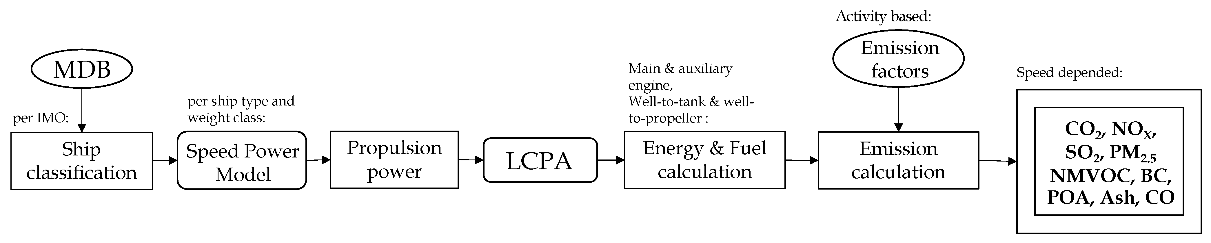
While there are some open-source maritime emissions models and inventories such as STEAM [11,12] and the IMO GHG Emissions Calculator [22], the inventory presented here addresses, in particular, the issues of transparency and reproducibility. Some inventories may not provide sufficient detail or transparency about their methodology or data sources, which may make it difficult for users to verify the accuracy of the estimates or compare the results with other studies.

The aim of this study was to provide a comprehensive data set of maritime emissions for the North Sea and Baltic Sea with scenario capabilities. The anonymization and interpolation of the data allow open-source publication as csv-files, to make them available to (non-)modelers for their own analysis of, e.g., the health effects of maritime emissions, the social costs of maritime transport, emission mitigation effects of alternative fuel scenarios, and shore-to-ship power supply. The study aims to provide a valuable tool for policymakers, researchers, and stakeholders to evaluate the environmental impact of maritime transport and to develop policies to reduce its negative effects.

3. Methods

3.1. Activity Data

The introduction of the AIS marked the beginning of digitization in the shipping industry. Since the end of 2004, it has been mandatory for every ship over 100 GT to be equipped with an AIS transmitter, which emits a signal every 6 s, providing, for example, the IMO identification number (unique identifier), the position (longitude/latitude), and a time stamp. Companies such as MarineTraffic, Vesselfinder, and IHS Fairplay collect and store these AIS signals and sell historical data. HELCOM (Baltic Marine Environmental Protection Commission) provide AIS data for the Baltic Sea region free of charge for research purposes. The presented emission inventory is based on high-temporal-resolution HELCOM [23] (Baltic Sea) and Vesselfinder [24] (North Sea) AIS data for 2015, covering the area between 65° N, −5° W, 48.3° S and 30.7° E, corresponding with the European Sulphur Emission Control Area (SECA). The AIS data for the Baltic Sea can be requested from HELCOM and are available for purchase from Vesselfinder for the North Sea.

3.2. Ship Routes

Consideration of shipping routes is an essential part of the emissions modeling of the shipping sector. Shipping routes can influence emission modeling by, inter alia, determining the type of fuels used, depending on the regulations and availability in the respective region. For the analyzed area, the SECA regulations apply.

Ship routes in the Baltic Sea and North Sea in 2015 were created from the acquired AIS data for all ships identified by their IMO number as being above 100 GT. Each route consists of segments that were formed from two consecutive AIS data points, using the following steps:

• Sorting of ship point data (longitude/latitude) by time stamp.
• Calculation of the distance between two consecutive time stamps using the Haversine equation.
• Calculation of the time duration between the two consecutive time stamps.
• Calculation of the speed of the ship between the time stamps based on time and distance.
• The spatial density of received AIS signals is significantly lower in the open sea than in coastal areas. To mitigate this, a method of rearrangement and interpolation to uniform 5 min time intervals of AIS signals is employed.
• When the calculated speed of a ship falls below 1 knot, the ship’s speed is set to 0 knots. This is done based on the assumption that the ship is neither docking nor maneuvering, and that only the auxiliary engine is active at such low speeds. By setting the ship’s speed to 0 knots in these situations, it is possible to differentiate between periods of inactivity and periods of slow movement, and accurately track the ship’s location and activity. This was confirmed by analysis of the AIS Vesselfinder data, as the navigational status was on average (as of June 2015) 0.7 knots (at anchor) and 0.4 knots (moored) [25].
• As a necessary simplification, any data points with a calculated speed greater than 15 m/s (equivalent to approximately 29 knots) are removed. This is done to address artifacts that may arise from erroneous longitude/latitude data, particularly when the time difference between two points is short but the distance between them is high, resulting in implausible vessel speeds. If a vessel departs from the area under analysis, the route calculation is interrupted, as it may not be possible to interpolate between two positions due to an extended route outside the area of interest, which could span several hours. The route calculation is also interrupted if the ship is at the edge of the area of interest and the distance between the calculated points is greater than 300 m. When the ship re-enters the area of interest, the route calculation is restarted. It is worth noting that ships may sometimes travel at speeds greater than 15 m/s, due to current effects. This factor is not accounted for in the presented model.

Figure 1 shows the annual gridded CO₂ emissions in the area under consideration. This initial result is a basic plausibility check for the bottom-up calculation of ship routes and emissions. The main and well-known shipping routes (cf. [26]) are clearly identifiable from the AIS-data-generated routes.

3.3. Ship Types and Characteristics

Decisive factors determining the emissions from individual ships are primarily the ship type, size, age, and engine configuration. The Maritime Data Base (MDB) hosted by Vesselfinder, which includes 18,309 IMO identification numbers in the given area, was used to cluster the ships using the listed AIS type [24] (The MDB offers a range of information for each IMO identification number: Name, Built (Year), Flag, Type (AIS-Type), Status, GT (Gross Tonnage), DWT (Deadweight tonnage), LOA (Length over all), LPP (Length between perpendiculars), Beam and Draft.). Based on the AIS ship types, standardized ship types, and the expertise of shipbuilders [27], nine generic ship types were classified in this study: CarCarrier, Container, RoRo, Bulker, RoPax, MPV (Multi Purpose Vessel), Tanker, Cruise, and Diverse (The ship class Diverse is mainly composed of 20% tugs, 25% fishing vessels and 16% offshore supply/tugs. Tugs have a high installed power, but rarely use it due to high berthing times (70–80%) and therefore are not defined as a separate class.). If the MDB did not specify the AIS type for a particular IMO identification number, the ship was assigned to the Diverse ship type. A statistical analysis of the MDB data provided the weight distribution within each ship type. Based on this and international ship sizes (weight classes), between two and four weight classes were defined per ship type. The Tanker and Container size classes are based on the international ship classes Handy Size (1), Handy Max (2), PanMax (3), and SuezMax (4).

Table 1. Ship characteristics in type and size (weight) classes 1–4, based on statistical analysis of the MDB [25] and ship building expertise [27].

Type	Unit 1	Main Engine 2	Auxiliary Engine	1	2	3	4
RoPax	GT	medium	medium	0–24,999	from 25,000
CarCarrier 3	GT	slow	medium	0–39,999	from 40,000
RoRo	GT	medium	medium	0–24,999	from 25,000
Cruise	GT	medium	medium	0–24,999	from 25,000
Diverse	GT	medium	medium	0–1999	from 2000
Container 4	GT	slow	medium	0–17,499	17,500–54,999	55,000–144,999	from 145,000
Tanker	DWT	slow	medium	0–34,999	35,000–49,999	50,000–119,999	from 120,000
Bulker	DWT	slow	medium	0–34,999	35,000–49,999	50,000–119,999	from 120,000
MPV	DWT	slow	medium	0–11,999	from 12,000

¹ Weight classes are measured in GT (gross tonnage) or DWT (dead weight tonnage), depending on the type of ship. ² Engine configuration differs between medium- or slow-speed diesel engines, depending on the type of ship. It is assumed that all ships within a particular class have the same engine configuration. ³ Typical size specifications for pure car carriers (PCC), in terms of the number of transported cars, was translated into GT. ⁴ Typical sizes of TEU (twenty foot equivalent unit, standard for container ships) or PanMax, SuezMax, etc., were translated into GT.

shows the set ship types by size class (weight classes) (1–4).

The ship types additionally differ in their engine configuration. A ship usually uses two sets of engines: the main engine(s), which provides the required propulsion power, and the auxiliary engine(s), which supply electrical power to the ship’s electrical system via generators [27]. Both engine sets run at different loads and have different engine characteristics and corresponding fuel consumption and associated emissions during operation. In general, a distinction is made between slow-speed, medium-speed, and high-speed diesel engines [28]. The decisive factor here is the engine speed. Slow-speed engines operate from 70 rpm up to 300 rpm, as is the case for most large two-stroke engines found on ships. Medium speed engines typically operate from approximately 300 rpm to 900 rpm [27].

3.4. Energy and Fuel Consumption

The required power for propulsion was calculated using a speed–power curve (SPC) per ship type and size class [27], which determines the power consumption of each ship type as a function of speed. The calculation determines the required propeller power $P_D$ [29]. The input variables are class-specific values, such as average length, width, and draft (arithmetic average of all ships with the set size class from the MDB). The SPC is simple to use and calibrate. It should be noted that the models represent generic, and thus average, ship types; the suitability of the application for modeling a single ship is dependent on the context and it is not intended.

The auxiliary engine in all ships is assumed to be a medium-speed diesel engine. For simplification, it is assumed that the auxiliary diesel power is essentially constant over all speeds [27]. Power values are based on EEDI specifications [1]. Even though the power can increase at higher speeds, due to, for example, seawater cooling or the operation of lube oil pumps, this effect should influence the overall results by less than 1% [27].

For the calculation of expended energy and fuel consumption, a proprietary life cycle performance analysis (LCPA) tool was used. The tool was developed jointly by the Flensburger-Schiffsbaugesellschaft Gmbh (FSG), BALance Technology Consulting, SSPA Sweden, Teknologian tutkimskeskus VTT, IFEU, and Det Norske Veritas [30,31], to support the generation of ship designs. The LCPA model is made available by BALance Technology Consulting and is available for purchase (LCPA). In the context of the present analysis, the LCPA was made available by the project partners of the FSG. The LCPA tool and SPC model were coupled to determine the fuel mass flow, which is calculated using the assumed power of the engine, together with the mechanical or electrical efficiencies and the specific fuel consumption for a certain time period. The energy expended was derived from the amount of fuel consumed and its calorific value (This step cannot be published, however can be traced and reproduced using the efficiency approximations of the ship’s engines and the calculated propeller power within the SPC) [31]. It is assumed that all ships use low-sulfur marine gas oil (LSMGO) (lower heating value (LHV) 42.675 kJ/kg) with a sulfur content of less than 0.1%, in line with IMO regulations within the European Sulphur Emission Control Area (SECA) [32].

3.5. Emission Calculation

Tank-to-propeller pollutant emissions are determined using activity-based emission factors that relate to the fuel or energy consumption, in combination with the navigational phase of the ship [33]. There are three navigation phases, as a distinction is made between underway, maneuvering, and hoteling/at berth (maneuvering and hoteling are often analyzed as one).

The calculation of NO_x, SO₂, PM_2.5, and CO₂ was performed within the LCPA model [31]. Due to the closed-source nature of the tool, only the qualitative calculation process is described. CO₂ emissions were calculated from the carbon fraction of the used fuel (LSMGO, 3206 t_CO2/t_fuel) [31]. SO₂ emissions were determined using the acidification potential, based on the fuel sulfur content (0.1%) and stoichiometric combustion to SO₂ in the energy converter [31]. PM emissions were calculated using the equation $\mathrm{PM}=0.2+0.6·S$ (g/kWh) for internal combustion engines [2,31], where S is the sulfur content of the fuel used. NO_x emissions were assumed to be in line with the official MARPOL tier regulations [2], depending on the ship construction date (see

Table 2. Nitrogen oxide guidelines in the North Sea and Baltic Sea ECA (Emission Control Area) according to the IMO [2], MARPOL Annex VI. n = engine’s rated speed in revolutions per minute (rpm).

		Total Weighted Cycle Emission Limit (g/kWh)
Tier	Ship Construction Date on or after	n < 130	n = 130–1999	n > 2000
I	1 January 2000	17.0	45 · n (−0.2)	9.8
II	1 January 2011	14.4	44 · n (−0.2)	7.7
III	1 January 2021	3.4	9 · n (−0.2)	2.0

). The Tier I guideline was assumed for all ships built before 2000 [34], as this was set close to the actual pollutant levels before 2000 [27].

POA, NMVOC, Ash, BC, and CO emissions were calculated using literature-based emission factors, together with the fuel or energy consumption determined within the LCPA tool. A variety of emission factors for maritime applications can be found in the literature [13,19,21,33,35,36,37,38]. A key study is EMEP CORINAIR, the Guidance Document for Air Pollutant Emissions Inventory published by the European Environment Agency (EEA) [39]. The 2019 version of the guide [33] provides activity-based emission factors for shipping (last update 12/2021 [37]). All of the emission factors used, as well as an extensive literature review of additional emission factors for sensitivity analyses related to engine types, are available in the Zenodo repository [40].

Speed-related emissions $e\left(v\right)$ in kg were calculated from selected emission factors $ef$ and E or F, the ship’s energy and fuel consumption, respectively, using Equations (1) and (2).

$$\begin{array}{c}\hfill e\left(v\right)=ef·E\left(v\right)\end{array}$$

(1)

$$\begin{array}{c}\hfill e\left(v\right)=ef·F\left(v\right)\end{array}$$

(2)

In addition to the activity-based (tank-to-propeller) emissions, the life cycle emissions of the fuel used (well-to-tank) were also analyzed. The LCPA tool provides well-to-tank emissions of NO_x, SO₂, PM_2.5, and CO₂ [31]. A full life cycle analysis can be used to evaluate the overall impact of a fuel, in terms of greenhouse gas and pollutant emissions, including all phases from production to use. The typical well-to-tank life stages of marine fuels include extraction, transportation, conversion, carriage, and bunkering. The LCPA software used the UMBERTO [41] life cycle software to determine the emission factors for well-to-tank emissions [30,31].

3.6. Processing

The introduced steps and data sets are brought together as follows. The individual steps can be traced in the publicly available code [29].

• Classification of each ship by IMO number, according to scenario-specific ship type and depending on age and scenario year, and unique assignment of the model via ship type and size class.
• Randomization of IMO numbers, in order not to be able to trace back to the proprietary AIS data.
• Integration of scenario-specific (e.g., year for NO_x regulation) models, including emissions and fuel consumption depending on speed.
• Calculation of all emissions, energy consumption, and related parameters for a 5 min interval, using interpolation based on the model’s supporting values and the average speed of the ship during each 5 min interval.
• Generation of an hourly georeferenced emission inventory for further analysis.

Figure 2 summarizes the methodological steps used to compile the inventory.

4. Data Description

All input and output data can be accessed via the Zenodo data repository [40]. The supporting model code is available on GitHub [29].

(1) The CSV file emission model includes hourly emission quantities (well-to-tank and tank-to-propeller) and energy expended for the speed of the specific vessel type and size.

• Type (column A): Ship type definition in three components separated by an underscore (_): (1) the ship type (see Table 1), (2) the size class 1–4 [40], and (3) the age-dependent NO_x regulation, Tier I, Tier II, or FS (future scenario, equivalent to Tier III), e.g., ropax_2_tier 1 represents a RoPax vessel in size class 2 (above 25,000 GT), which was built before 01/01/2011.
• Engine (column B): Propulsion (main) engine or lectric (auxiliary engine) of a ship.
• Speed (m/second) (column C): The calculated speed over ground of a ship.
• Energy (well-to-tank) (J) (column D): Energy expended for the production, transportation, and distribution of the fuel used for propulsion.
• Pollutant (well-to-tank) (kg) (columns E–H): CO₂, SO_x, NO_x and PM emissions during production, transportation, and distribution of the fuel consumed (for SQ-2015 LSMGO).
• Energy (J) (column I): Energy expended for the propulsion of the ship per speed.
• Fuel Consumption (kg) (column J): Tank-to-propeller fuel consumption.
• Pollutant (kg) (columns K-S): Tank-to-propeller emission of CO₂, SO_x, NO_x, PM, BC, ASH, POA, CO, and NMVOC.

(2) The emission inventory ship_emissions_YYYYMMDD is available as 396 csv files, one for each day in 2015 and December 2014. These contain the following data records:

• UniqueID (column A): Unique identifier of ship. Due to the use of proprietary input data (AIS), the originally used unique identifier (IMO-number) was replaced with a random number.
• Type (column B): See the description for type in the emission model input descriptor list above.
• Datetime (column C): Date and time stamp following the format YYYY-DD-MM HH:MM:SS.
• Lat (column D): Calculated latitudinal position of the ship in decimal degrees.
• Lon (column E): Calculated longitudinal position of the ship in decimal degrees.
• Speed_calc (column F): Calculated speed in m/s from the calculated distance at a 5 min time interval.
• Propulsion-Energy (Well to tank) (J) (column G): Energy expended for the production, transportation, and distribution of the fuel used in the main engine.
• Electrical-Energy (Well-to-tank) (J) (column H): Energy expended for the production, transportation, and distribution of the fuel used in the auxiliary engine.
• Propulsion-Pollutant (Well-to-tank) (kg) (columns I, K, M, and O): CO₂, SO_x, NO_x, and PM (PM_2.5) emissions from the production, transportation, and distribution of the fuel needed by the main engine for propulsion in the respective time interval.
• Electrical-Pollutant (Well to tank) (kg) (columns J, L, N, and P): CO₂, SO_x, NO_x, and PM (PM_2.5) emissions from the production, transportation, and distribution of the fuel needed by the auxiliary engine in the respective time interval.
• Propulsion-Energy (J) (column Q): Energy content of the fuel used for propulsion (tank-to-propeller) of the main engine in the respective time interval.
• Electrical-Energy (J) (column R): Energy content of the fuel used for the auxiliary engine (tank-to-propeller) in the respective time interval.
• Propulsion-Fuel Consumption (kg) (column S): Fuel consumption for the propulsion (main engine) of the vessel in the respective time interval.
• Electrical-Fuel Consumption (kg) (column T): Fuel consumption for the hoteling load (auxiliary engine) of the vessel in the respective time interval.
• Propulsion-Pollutant (kg) (columns U, W, Y, AA, AC, AE, AG, AI, and AK): CO₂, SO_x, NO_x, PM, BC, ASH, POA, CO, NMVOC emissions from the main engine during operation (tank-to-propeller) of the ship.
• Electrical-Pollutant (kg) (columns V, X, Z, AB, AD, AF, AH, AJ and AL): CO₂, SO_x, NO_x, PM, BC, ASH, POA, CO, NMVOC emissions from the auxiliary engine during operation (tank-to-propeller) of the ship.

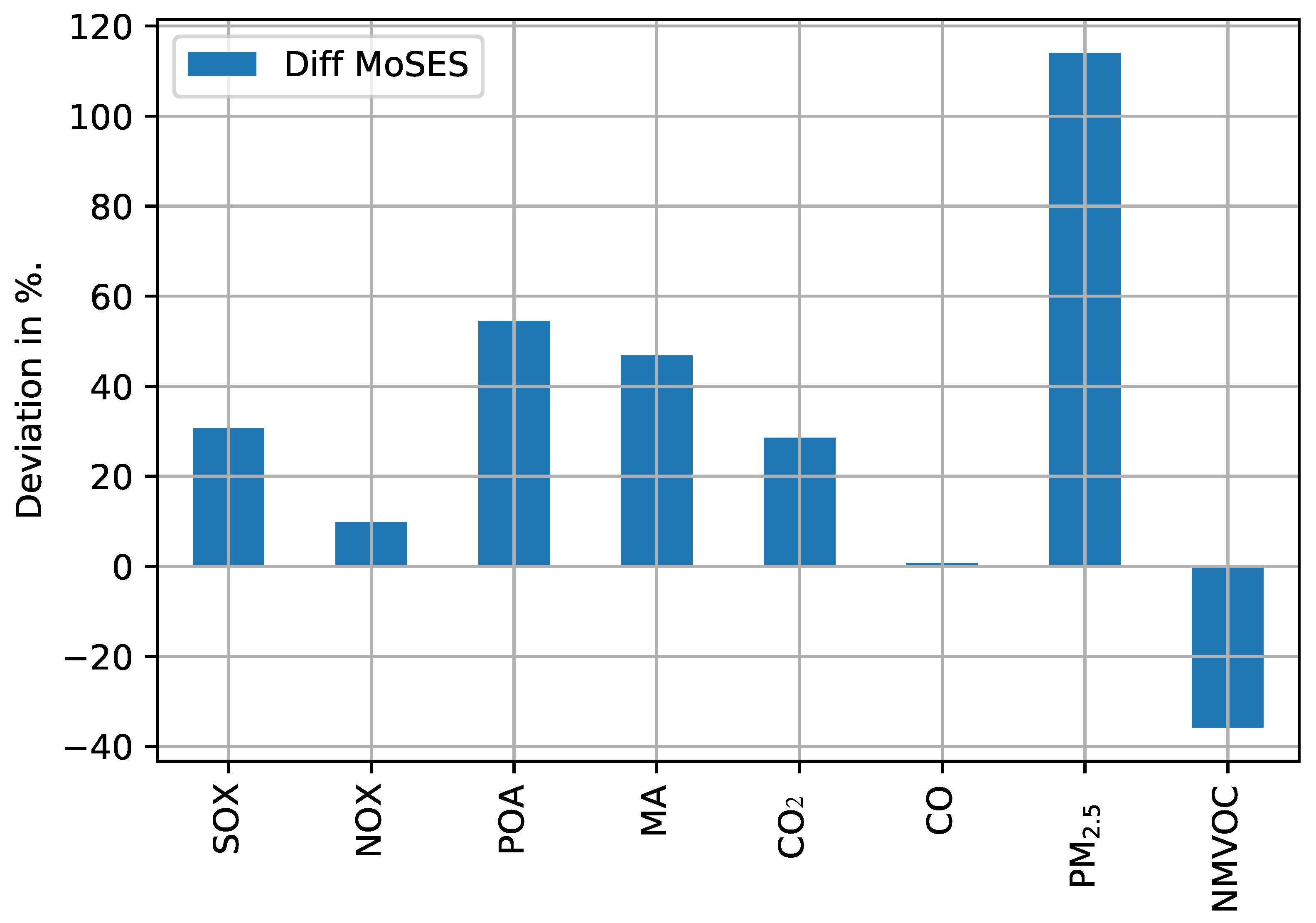
(3) In the interest of transparency and reproducibility, a number of supporting data sets are available on Zenodo [40]. The speed-power-model.xlsx file summarizes the assumed power (kW) for the main and auxiliary engines, as well as inputs for the SPC calculation (length (m), width (m), drauft (m), the shape-dependent variable c_b, the propulsion efficiency, and the wetted surface of the ship in m² specific to speed, ship type, and weight class. The emission_factors.xlsx file summarizes the emission factors specific to engine type, navigation phase, and pollutant, as well as an extensive, referenced list of factors for sensitivity analyses. The analysis.xlsx file contains additional information for further analyses of, for example, emission quantities as assessed within different models for cross-model comparisons. Additionally included is the time spent at a particular speed, as well as the number of ships considered in each ship and weight class. The supplementary_material.pdf file summarizes regulations and targets for maritime emissions [1,2]. This file also contains the equations used to calculate the propulsion power $P_D$.

(4) All related code, including static input data, is available on GitHub [29]. Within the folder emission_model, the maximum_speed_per_type.csv file lists the maximum possible speed in m/s [27]. The ship_weightclass_mapper.csv file assigns the different ship types and sizes to weight types (DWT or GT) and the lower and upper bounds of the weight classes connecting Tier I, II, and FS with the year of construction and the typical engine rpm for each specification. Both the ship_type_fsg_mdb_mapper.xlsx file and short_long_name_mapper.xlsx file are used for the preprocessing of ship type classification. Within the folder lcpa-models are SensitivityAnalysis-ShipeTypeName-Rev2.csv files, which are hourly emission models for all ship types and sizes. The scr folder contains the model code itself, preprocessing steps and routines for result and input data analyses.

5. Validation

Comparison with Existing Emission Inventories

Crucial in the creation of an emissions inventory through bottom-up modeling is the validation of the results obtained. There was no possibility of comparing the chosen assumptions and related results with actual emission measurements. Initial studies on measuring ship emissions using drones are underway [42], exemplified by the SCIPPER project [43] and efforts by the European Maritime Safety Agency (EMSA). However, only individual ships on a specific voyage can be measured. A cross-model comparison, however, allows a statement about the quality of the obtained results. Useful in this context are the MoSES [21] and STEAM models [13]. The two models have been used to create emission inventories for the North Sea and Baltic Sea area: MoSES [21] for 2015, STEAM—in this application—for 2011 [13].

Table 3. Result values from MoSES [21], STEAM [13], and the EUF inventory in Gg per year and respective deviations from the EUF results in %.

	MoSES	EUF	STEAM	Diff MoSES (%)	Diff STEAM (%)
Year	2015	2015	2011
Number of Ships	21,845	16,632	n/a	23.86	n/a
SO2	32.55	24.90	192.10	30.70	671.34
NOx	897.97	818.00	806.20	9.78	−1.44
BC	13.89	0.44	n/a	3036.76	n/a
POA	17.96	11.62	n/a	54.50	n/a
MA	0.32	0.22	n/a	46.85	n/a
CO2	44,886.43	34,931.98	35,740.00	28.50	2.31
CO	38.31	38.04	57.30	0.72	50.64
PM2.5	29.83	13.94	38.30	113.98	174.74
NMVOC	11.12	17.32	n/a	−35.81	n/a

summarizes the emission quantities, reference year, and number of ships analyzed for these two inventories and the presented results of the EUF inventory.

In general, a good agreement can be observed between the values from EUF, STEAM, and MoSES for most pollutants. The emission quantities from the STEAM and MoSES inventories tended to be higher than those from the EUF model. This can be explained, among other things, by the number of ships investigated in the area under consideration. Comparing the EUF and STEAM values, it can be seen that there was a significant deviation in SO_x emissions. This was largely due to the introduction of the 0.1% sulfur guideline in 2015, which can also partially explain the deviation in PM_2.5 emission results, as the reduced sulfur content in the fuel also reduced particulate matter emissions. Further comparative analyses are possible based on Hilpert et al. [40].

Figure 3 depicts a detailed comparison of emissions from the EUF and MoSES [21] inventory and the deviations of the results of MoSES from the EUF emission inventory in percent. There was a tendency for MoSES emission values to be higher than those in the EUF inventory, which may have been due to the number of ships considered and the different calculation approaches for energy consumption and related emissions. A comprehensive comparison of the selected fuel and energy modeling would be difficult, due to the different methodological paths chosen. However, CO₂ emissions are a stable indicator, since the carbon from the required fuel burns almost entirely to CO₂. The variation here is consistent with the variations in the number of ships considered. The SO₂ emissions are in the same order of magnitude for the MoSeS and EUF values. The differences in NO_x, POA, and Ash are within a reasonable range and can be justified by the different emission factors used. The differences in NMVOC and BC are striking. Contrary to the general trend, NMVOC emissions are higher in the EUF inventory. BC emissions, on the other hand, are an order of magnitude lower in the EUF emission inventory.

The EUF model mainly uses fuel-based emission factors, while the emission factors within MoSES are related to the energy expended. MoSES uses a factor of 0.03 g/kWh for BC emissions from the main engine and 0.15 g/kWh for the auxiliary engine, as well as a adjustment of the factor to low loads of the engine. The EUF model uses the EEA’s [37] factors (see

Table 4. Emission factors used in MoSES [21] and EUF, FSC = fuel sulfur content (0.1%) and SFOC = specific fuel oil consumption.

Model	BC	POA	Ash	CO	NMVOC
MoSES	0.03 g/kWh	0.2 g/kWh	FSC · SFOC · 0.02 g/kWh	0.54 g/kWh	0.5 g/kWh
EUF	0.0329 kg/t	0.09 g/kWh	0.0002 kg/t	3.47 kg/t	1.52 kg/t

). A more in-depth analysis that examines variances arising from energy expenditure is recommended.

The analysis of the different values from STEAM, MoSES, and EUF show how crucial the choice of emission factors is. The factors for the EUF model were chosen based on an extensive literature review; particular emphasis was placed on the timeliness of the source. Nevertheless, there are large uncertainties that must be taken into account when interpreting the obtained results.

6. Discussion

Uncertainties

The results of this study must be viewed critically with regard to the methods and models used. The results are discussed concerning (1) (input) data (quality), and (2) the general modeling approach and connected assumptions.

(1) Uncertainties about the reliability of the emission inventories arise from the use of the closed-source LCPA model and raw AIS data, which are proprietary. This limits the reproducibility and transparency of the values generated. The creation of ship routes is influenced by the quality of the AIS data used and by the interpolation routines chosen. The AIS data used have a high data ranking (A or B are most accurate [24]), which makes the generated values more reliable. Since the end of 2018, satellite-processed AIS data are available, which can further increase the accuracy of results. Additionally, climate change may affect shipping routes by altering ocean currents and sea levels, and changing weather patterns. For example, changes in ocean currents could affect the efficiency of shipping routes, while rising sea levels could require modifications to port facilities and coastal infrastructure [44].

The LCPA model is a closed-source model. However it builds on the expertise of ship builders and environmental analysts. The emission values and associated calculation steps used within the LCPA model can be traced with sufficient accuracy.

(2) Within the general study approach, the chosen speed reduction criteria may also affect the results. Unlike other studies, such as used within the MoSES model [21], this study does not consider engine load for the calculation of fuel and power consumption. The speed–power curves take this into account, but the auxiliary engine is only partially responsive to the engine load and is simplified for modeling purposes. Unlike STEAM [11,12], the influence of waves and currents is not directly considered in the EUF model. However, the SPCs tend to have high power assumptions, so consideration of waves and currents was not considered essential. The loading condition of ships was not considered in the studies analyzed, such as [11,21]. Although some shipping companies may provide access to real-time data, this is often treated as confidential and not publicly available. As a result, the loading condition is not taken into account during the EUF analysis.

Generic ship types were defined, based on a complementary data set obtained from Vesselfinder, which can be compared with the AIS types from Vesselfinder [24]. Nevertheless, the integration of a more accurate ship type assignment system could further refine the emission values. Additionally, only ships over 100 GT were utilized in the EUF model, so the study does not provide an assessment of all emissions.

For future scenarios, fleet developments have to be taken into account. In 2017, maritime transport accounted for nearly 90% of international trade measured in tonne-kilometers [28]. Maritime trade volumes have tripled since 1980. The DNV expects seaborne trade to be 35% higher in 2030 than in 2017 and to increase by a further 12% before 2040. The UNCTAD [45] projected an average annual growth of 3.5% between 2019 and 2024, with the largest relative growth expected in the gas and container cargo sectors, each increasing by 135–150%. Bulk carriers are projected to increase by 40% by 2050, based on a combination of an increase in non-coal bulk trade and a possible reduction in coal shipments [45]. Looking specifically at the future development of container ships and their contribution to total emissions, it can be assumed that future emissions will increase disproportionately to the increase in goods transported.

7. Further Use of Data, Data Availability and User Notes

The data in the EUF emission inventory can be used to assess air pollution regulations and incorporate different emission control or propulsion technologies. The data can also be used in chemical transport modeling, to evaluate the air pollutant concentration resulting from maritime emissions. Subsequently, gridded population data could be used together with the results from chemical transport modeling to estimate the human health impacts of air pollutants. As the EUF inventory also provides fuel and energy consumption at a high resolution, new emission factors could be applied for different pollutants and the inventory could be expanded accordingly. The high spatial resolution of the data set makes it possible to analyze the shore-to-ship power demand for renewable energy to reduce emissions from the auxiliary engine at berth.

The code for the underlying calculations and post-processing functions are available under the BSD 3-Clause license [29]. The analysis uses Python as a programming language.

The emission inventory and all supporting data sets, with the exception of the AIS data, are available under an open license on Zenodo [40]. The data can be processed using Excel or any other data processing software capable of processing csv files, such as Python or R.

AIS data for the Baltic Sea can be obtained from HELCOM via a data agreement. The AIS data for the North Sea is proprietary data, which can be purchased from Vesselfinder. The LCPA model used is also proprietary, but the associated computational pathways are described qualitatively, allowing sufficient traceability of the results.

References

1. International Maritime Organization. Fourth IMO Greenhouse Gas Study 2020; Technical Report; IMO: London, UK, 2020. [Google Scholar]
2. International Maritime Organization. Third IMO Greenhouse Gas Study 2014; Technical Report; IMO: London, UK, 2015. [Google Scholar]
3. BMWK. Verordnung über Netzentgelte bei der Landstromversorgung und zur Redaktionellen Anpassung von Vorschriften im Regulierungsrecht; Verordnung 52; Bundesministerium für Wirtschaft und Energie: Bonn, Germany, 2019. [Google Scholar]
4. Corbett, J.J.; Fischbeck, P. Emissions from Ships. Science 1997, 278, 823–824. [Google Scholar] [CrossRef]
5. Corbett, J.J.; Fischbeck, P.S.; Pandis, S.N. Global nitrogen and sulfur inventories for oceangoing ships. J. Geophys. Res. 1999, 104, 3457–3470. [Google Scholar] [CrossRef]
6. Corbett, J.J.; Koehler, H.W. Considering alternative input parameters in an activity-based ship fuel consumption and emissions model: Reply to comment by Øyvind Endresen et al. on “Updated emissions from ocean shipping”: Commentary. J. Geophys. Res. 2004, 109, D23. [Google Scholar] [CrossRef]
7. Corbett, J.; Ruwet, M.; Xu, Y.C.; Weller, P. Climate governance, policy entrepreneurs and small states: Explaining policy change at the International Maritime Organisation. Environ. Politics 2020, 29, 825–844. [Google Scholar] [CrossRef]
8. Eyring, V. Emissions from international shipping: 1. The last 50 years. J. Geophys. Res. 2005, 110, D17305. [Google Scholar] [CrossRef]
9. Van der Tak, C.; Cotteleer, A. Emissions 2009: Netherlands Continental Shelf, Port Areas and Ospar Region II; MARIN: Wagenigen, The Netherlands, 2011. [Google Scholar]
10. Van der Gon, H.D.; Hulskotte, J. Methodologies for Estimating Shipping Emissions in the Netherlands—A Documentation of Currently Used Emission Factors and Related Activity Data; Technical Report 500099012; Netherlands Environmental Assessment Agency: Bilthoven, The Netherlands, 2010. [Google Scholar]
11. Jalkanen, J.P.; Johansson, L.; Kukkonen, J. A Comprehensive Inventory of the Ship Traffic Exhaust Emissions in the Baltic Sea from 2006 to 2009. AMBIO 2014, 43, 311–324. [Google Scholar] [CrossRef] [PubMed]
12. Jalkanen, J.P.; Johansson, L.; Kukkonen, J.; Brink, A.; Kalli, J.; Stipa, T. Extension of an assessment model of ship traffic exhaust emissions for particulate matter and carbon monoxide. Atmos. Chem. Phys. 2012, 12, 2641–2659. [Google Scholar] [CrossRef]
13. Jalkanen, J.P.; Johansson, L.; Kukkonen, J. A comprehensive inventory of ship traffic exhaust emissions in the European sea areas in 2011. Atmos. Chem. Phys. 2016, 16, 71–84. [Google Scholar] [CrossRef]
14. Johansson, L.; Jalkanen, J.P.; Kalli, J.; Kukkonen, J. The evolution of shipping emissions and the costs of recent and forthcoming emission regulations in the northern European emission control area. Atmos. Chem. Phys. Discuss 2013, 13, 16113–16150. [Google Scholar] [CrossRef]
15. Johansson, L.; Jalkanen, J.P.; Kukkonen, J. Global assessment of shipping emissions in 2015 on a high spatial and temporal resolution. Atmos. Environ. 2017, 167, 403–415. [Google Scholar] [CrossRef]
16. Kramel, D.; Muri, H.; Kim, Y.; Lonka, R.; Nielsen, J.B.; Ringvold, A.L.; Bouman, E.A.; Steen, S.; Strømman, A.H. Global Shipping Emissions from a Well-to-Wake Perspective: The MariTEAM Model. Environ. Sci. Technol. 2021, 55, 15040–15050. [Google Scholar] [CrossRef] [PubMed]
17. Karl, M.; Jonson, J.E.; Uppstu, A.; Aulinger, A.; Prank, M.; Sofiev, M.; Jalkanen, J.P.; Johansson, L.; Quante, M.; Matthias, V. Effects of ship emissions on air quality in the Baltic Sea region simulated with three different chemistry transport models. Atmos. Chem. Phys. 2019, 19, 7019–7053. [Google Scholar] [CrossRef]
18. CNSS. Clean North Sea Shipping—Key Findings and Recommendations; Final Report; Clean North Sea Shipping: Newcastle upon Tyne, UK, 2014. [Google Scholar]
19. Aulinger, A.; Matthias, V.; Zeretzke, M.; Bieser, J.; Quante, M.; Backes, A. The impact of shipping emissions on air pollution in the greater North Sea region—Part 1: Current emissions and concentrations. Atmos. Chem. Phys. 2016, 16, 739–758. [Google Scholar] [CrossRef]
20. Matthias, V.; Aulinger, A.; Backes, A.; Bieser, J.; Geyer, B.; Quante, M.; Zeretzke, M. The impact of shipping emissions on air pollution in the greater North Sea region—Part 2: Scenarios for 2030. Atmos. Chem. Phys. 2016, 16, 759–776. [Google Scholar] [CrossRef]
21. Schwarzkopf, D.A.; Petrik, R.; Matthias, V.; Quante, M.; Majamäki, E.; Jalkanen, J.P. A ship emission modeling system with scenario capabilities. Atmos. Environ. X 2021, 12, 100132. [Google Scholar] [CrossRef]
22. IMO. Excel, International Maritime Organization. 2012. Available online: https://greenvoyage2050.imo.org/fleet-and-co2-calculator/ (accessed on 3 March 2023).
23. HELCOM. Emissions from Baltic Sea Shipping 2006–2018; MARITIME 19-2019 5-2; HELCOM: Lisbon, Portugal, 2019. [Google Scholar]
24. Vesselfinder. AIS Ship Types—AIS Data. 2022. Available online: https://www.vesselfinder.com/ (accessed on 23 April 2023).
25. Vesselfinder. Available online: https://www.vesselfinder.com/historical-ais-data (accessed on 23 March 2023).
26. EC. Baltic Sea Shipping Traffic Intensity. 2017. Available online: https://maritime-spatial-planning.ec.europa.eu/practices/baltic-sea-shipping-traffic-intensity (accessed on 23 April 2023).
27. Nagel, R.; Flensburger Schiffbau-Gesellschaft mbH & Co KG, Flensburg, Germany; Dettner, F.; Europa University Flensburg, Flensburg, Germany. Shipbuilding Expertise. Personal communication, 2021.
28. DNV-GL. Martime Forecast to 2050; Forecast; DNV GL: Høvig, Norway, 2017. [Google Scholar]
29. Hilpert, S. znes/KlimaSchiff: V1.0 (V1.0); Zenodo, Source Code, BSD 3-Clause; Europa Universität: Flensburg, Germany, 2022. [Google Scholar] [CrossRef]
30. Thiem, C.; Liebich, A.; Münter, D. Joules—Fuel Data Report, Identification, Physico-Chemical Properties and Well-To-Tank Data of Marine Fuels; Confidential Report FP7-SST-2013-RTD-1; Flensburger Schiffbau-Gesellschaft mbH & Co KG: Hamburg, Germany, 2013. [Google Scholar]
31. Joules. LCPA Tool incl. LCPA and LCA Description; Confidential Report 21-1; Flensburger Schiffbau-Gesellschaft mbH & Co KG: Flensburg, Germany, 2014. [Google Scholar]
32. International Maritime Organization (IMO). Safety for Gas-Fuelled Ships—New Mandatory Code Enters into Force; IMO: London, UK, 2017. [Google Scholar]
33. European Environment Agency (EEA). EMEP/EEA Air Pollutant Emission Inventory Guidebook 2019—Technical Guidance to Prepare National Emission Inventories; EEA: Copenhagen, Denmark, 2019. [Google Scholar]
34. IMO. Nitrogen Oxides (NOx)—Regulation 13; IMO: London, UK, 2020. [Google Scholar]
35. Kristenen, H.O. Energy demand and exhaust gas emissions of marine engines. Clean Shipp. Curr. 2012, 1, 18–26. [Google Scholar]
36. Jun, P.; Gillenwater, M.; Barbour, W. CO2, CH4, and N2O Emissions from Transportation-Water-Borne-Navigation; Technical Report; IPCC: Geneva, Switzerland, 2001. [Google Scholar]
37. EEA. Emission Inventory International—1.A.3.d Navigation (Shipping) 2019, Update Dec. 2021; Guidebook 2019 SNAP 08042-4; EEA: Copenhagen, Denmark, 2021. [Google Scholar]
38. Entec UK Limited. Quantification of Emissions form Ships Associated with Ship Movements between Ports in the European Community; Final Report; Entec UK Limited: Northwich, UK, 2002. [Google Scholar]
39. EEA. EMEP/CORINAIR Emission Inventory Guidebook; EEA: Copenhagen, Denmark, 2007. [Google Scholar]
40. Hilpert, S.; Dettner, F.; Nagel, R. Emission Inventory of maritime Shipping on the Baltic and North Sea in 2015 with scenario capabilities. arXiv 2022, arXiv:2211.13129. [Google Scholar]
41. ifu hamburg. 2022. Available online: https://www.ifu.com/de/umberto/oekobilanz-software (accessed on 3 March 2023).
42. Winnes, H.; Moldanová, J.; Anderson, M.; Fridell, E. On-board measurements of particle emissions from marine engines using fuels with different sulphur content. Proc. Inst. Mech. Eng. Part J. Eng. Marit. Environ. 2016, 230, 45–54. [Google Scholar] [CrossRef]
43. SCIPPER. SCIPPER—Shipping Contributions to Inland Pollution Push for the Enforcement of Regulations; Horizon2020; SCIPPER: Brussels, Belgium, 2021. [Google Scholar]
44. DOT. The Potential Impacts of Climate Change on Transportation; Summary and Discussion Paper; DOT Center for Climate Change and Environmental Forecasting: Washington, DC, USA, 2002. [Google Scholar]
45. UNCTAD. Review of Maritime Transport; Technical Report; United Nations Conference on Trade and Development: New York, NY, USA, 2019. [Google Scholar]
Figure 1. CO2 emissions in kg in the North Sea and Baltic Sea for January and July, 2015.
Data 08 00085 g001
Figure 2. Schematic overview of the methodological steps utilized in the development of the EUF emission inventory, displaying the relevant processing steps within the square boxes. The input data for each step are contained within the circles and squares with rounded corners, the final output is shown in the double square. MDB = Maritime Data Base, LCPA = life cycle performance assessment.
Data 08 00085 g002
Figure 3. Deviation (in %) of values (emission quantity in the EUF inventory) to MoSES [21] for SQ-2015. MA = mineral ash.
Data 08 00085 g003