Article

CyL-GHI: Global Horizontal Irradiance Dataset Containing 18 Years of Refined Data at 30-Min Granularity from 37 Stations Located in Castile and León (Spain)

by
Llinet Benavides Cesar
*,
Miguel Ángel Manso Callejo
,
Calimanut-Ionut Cira
and
Ramon Alcarria
Departamento de Ingeniería Topográfica y Cartográfica, Escuela Técnica Superior de Ingenieros en Topografía, Geodesia y Cartografía, Universidad Politécnica de Madrid, Calle Mercator, 2, 28031 Madrid, Spain
*
Author to whom correspondence should be addressed.
Submission received: 13 December 2022 / Revised: 8 March 2023 / Accepted: 23 March 2023 / Published: 26 March 2023

Abstract

:
Accurate solar forecasting lately relies on advances in the field of artificial intelligence and on the availability of databases with large amounts of information on meteorological variables. In this paper, we present the methodology applied to introduce a large-scale, public, and solar irradiance dataset, CyL-GHI, containing refined data from 37 stations found within the Spanish region of Castile and León (Spanish: Castilla y León, or CyL). In addition to the data cleaning steps, the procedure also features steps that enable the addition of meteorological and geographical variables that complement the value of the initial data. The proposed dataset, resulting from applying the processing methodology, is delivered both in raw format and with the quality processing applied, and continuously covers 18 years (the period from 1 January 2002 to 31 December 2019), with a temporal resolution of 30 min. CyL-GHI can result in great importance in studies focused on the spatial-temporal characteristics of solar irradiance data, due to the geographical information considered that enables a regional analysis of the phenomena (the 37 stations cover a land area larger than 94,226 km2). Afterwards, three popular artificial intelligence algorithms were optimised and tested on CyL-GHI, their performance values being offered as baselines to compare other forecasting implementations. Furthermore, the ERA5 values corresponding to the studied area were analysed and compared with performance values delivered by the trained models. The inclusion of previous observations of neighbours as input to an optimised Random Forest model (applying a spatio-temporal approach) improved the predictive capability of the machine learning models by almost 3%.
Dataset License: CC-BY-SA-NC

1. Introduction

In solar forecasting, like any other research field, access to data is a primary factor in the discovery process, and the open publication of the datasets and methodologies used by authors in their studies is encouraged [1,2]. Lately, tools have been developed to facilitate access to publicly available solar data [3,4], and public institutions are increasingly providing their data [5,6]. However, as this is not always possible, created datasets are often private, or there are strong limitations on their use and distribution, and the number and quality of published irradiance datasets are still insufficient when compared to other research fields where large-scale datasets can be found in known repositories such as UC Irvine Machine Learning Repository (UCI) [7], Kaggle [8], and Linked Open Data Cloud [9].
In relation to published datasets for solar forecasting, references can be made to the source of the data provided such as store photovoltaic (PV) data [10], data collected by meteorological stations [11,12], and to the datasets resulting from the combination of several sources [13,14,15]. There are also datasets that accumulate data from many years [11,16], or datasets that take into account a larger number of measurement sites [10,17]. In this regard, Bright et al. [10] published a dataset containing photovoltaic system power measurements and metadata from 1287 PV systems located in three Australian states with a temporal granularity of ten min, and, although it features a high number of sites, it contains only seven months of data. The source of this data is a website where owners shared data on PV power generation using automated data loggers. Pedro et al. [13] proposed a dataset using data outputs from four different sources, namely, ground-based measurements, satellite-imagery features, sky-camera images, and numerical weather prediction for a selected site in Folsom, California. This dataset contains data for three years (2014 to 2016), with a temporal granularity of one min. Driemel et al. [11] provided high-quality ground-based radiation measurements in one-minute resolution collected by 59 stations, scattered around the world, from 1992 to 2017, from the Baseline Surface Radiation Network (BSRN). The proposed dataset is suitable for point analysis, but not for studies considering the spatial component, because the stations are not concentrated in a single site, and the different groups or organisations controlling the stations might apply distinct quality control procedures.
However, solar forecasting has a spatio-temporal characteristic, which has recently been studied in more detail by researchers in the field [18,19,20,21,22,23,24], and we believe that, in order to study the variability of radiation with respect to the spatial component, datasets with a wide spatial representation are needed.
In Spain, the databases with the greatest spatial distribution in the territory are maintained by the Meteorology State Agency (Spanish: Agencia Estatal de Meteorología, or AEMET) [25] and the Agroclimatic Information System for Irrigation (Spanish: Sistema de Información Agroclimática para el Regadío, or SIAR) [26]. Data from the Spanish SIAR network have been used in previous studies; for example, data from the Community of Castile and León has been used by Rodriguez et al. [27] to study four spatial interpolation methods over large areas with few measurement points. The authors used four AEMET stations as a reference to evaluate the quality of the results, and the Universal Kriging method, which considered the metrics evaluated, yielded the best results. Eschenbach et al. [28] used data from the SIAR network of the region of Castile and León to compare and evaluate the spatio-temporal characteristic. They compared a region with a high dispersion of sensors (the SIAR network of the region of Castile and León) versus a region with a high concentration of sensors (OAHU Solar Measurement Grid from National Renewable Energy Laboratory in the United States). The authors employed four machine learning models and obtained a forecast skill between 13% and 70%, concluding that the sensor network density, time resolution, and lead-time of the dataset have an important effect on the skill forecast of the model. Gutierrez-Corea et al. [29] used data from ten stations from the SIAR network from the Community of Castile and León to forecast solar irradiance and evaluate the influence of data from neighbouring stations to improve accuracy. The authors applied an artificial neural network that obtained the best results for the short-term horizon using information from the neighbours.
Of these two databases (AEMET, SIAR), Urraca et al. [30] point out that AEMET is the most reliable database, due to the quality of the devices used to make the measurements and, above all, due to the quality control to which the data are subjected; however, its stations are more dispersed and its access is restricted. In contrast, the SIAR network meets two important criteria: (1) it is highly representative throughout the Spanish territory, and (2) provides data in an open way, allowing access to its historical data, although the quality of its data is lower because the measuring devices are of lower quality. In addition, there are also regional databases such as Meteo Navarra (from the Spanish region of Navarra), Meteocat (Catalonia), Euskalmet (Basque Country), MeteoGalicia (Galicia), SIAR Rioja, and SOS Rioja [30].
In this paper, data from the SIAR network of the region of Castile and León (Spanish: Castilla y León, or CyL), managed by CyL’s Institute of Agricultural Technology [31] or ITACyL (ITA references the Spanish: Instituto Tecnológico Agrario), was chosen for the preparation of a dataset. The objective was to describe the methodology applicable to create a dataset of Global Horizontal Irradiance (GHI) that could be used in solar forecasting, with a wide spatial distribution, important for designing a spatio-temporal analysis, using openly available meteorological data captured for agricultural purposes. Furthermore, experiments for obtaining baseline performance values of optimised machine learning (ML) algorithms were carried out, and an improvement of almost 3% was observed in the forecast skill when considering the spatial component in the training.
The contributions of the research carried out is summarised as follows.
  • A dataset of public irradiance, CyL-GHI, is introduced, and the methodology applied to create it is described in detail.
  • Three popular artificial intelligence algorithms were optimised and tested on CyL-GHI; their performance values being offered as baselines to compare other forecasting implementations. Furthermore, the ERA5 values corresponding to the studied area were analysed and compared with performance values delivered by the trained models.
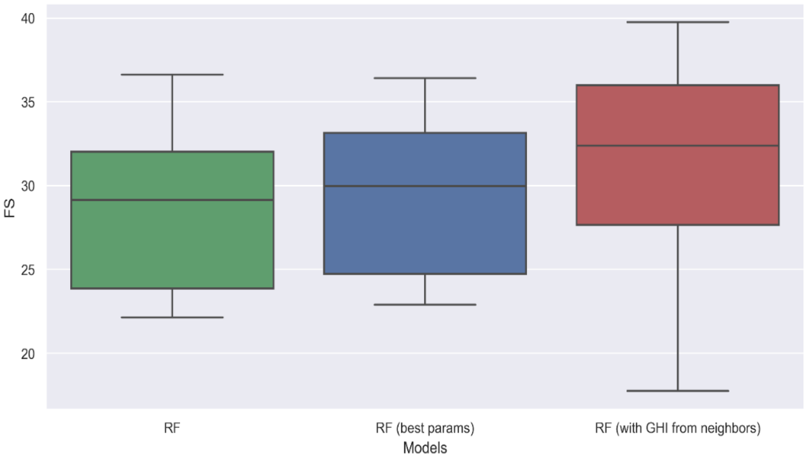
  • The inclusion of previous observations of neighbours as input to an optimised Random Forest model (by applying a spatio-temporal approach) improved the predictive capability of the machine learning models by almost 3%, indicating the importance of approaching the irradiance prediction task considering the spatial component.
The value of the presented dataset, named CyL-GHI, resides in:
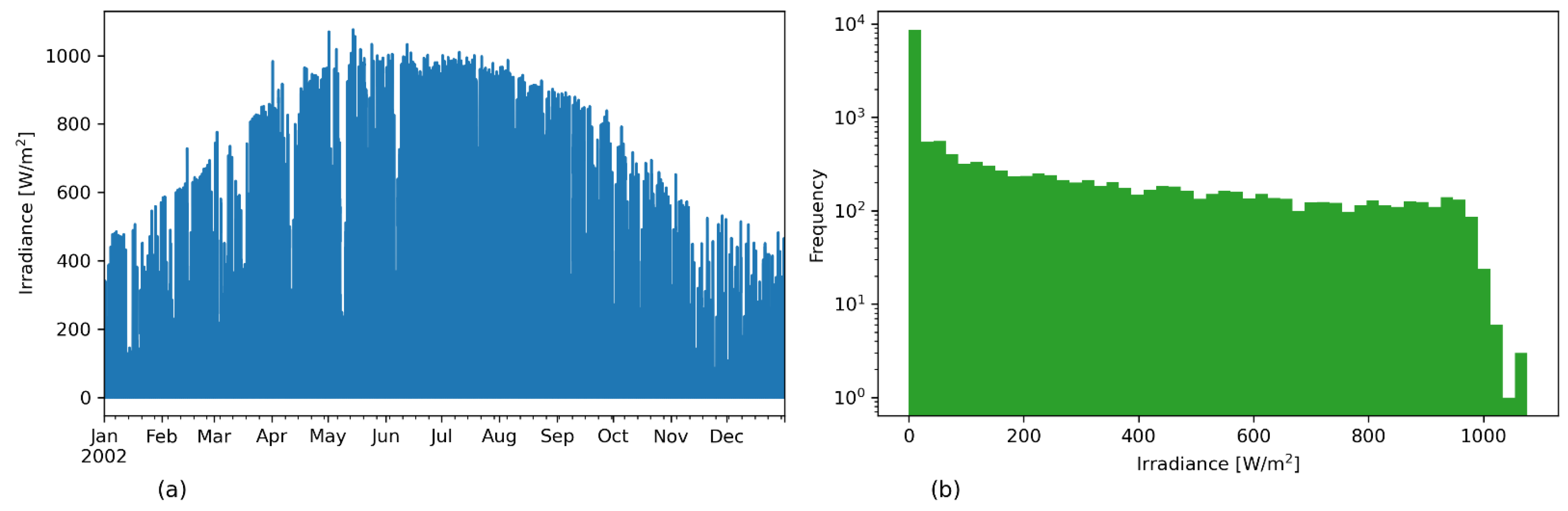
  • Its temporal representation, because it presents irradiance data for an 18-year period from January 2002 to December 2019 with a temporal resolution of 30 min.
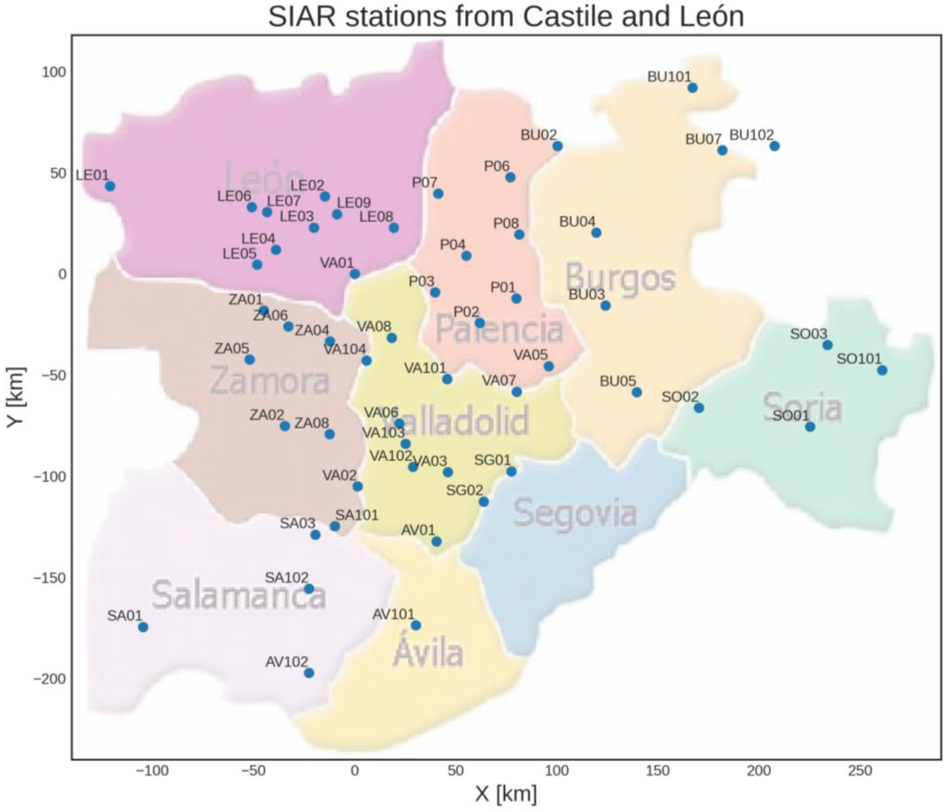
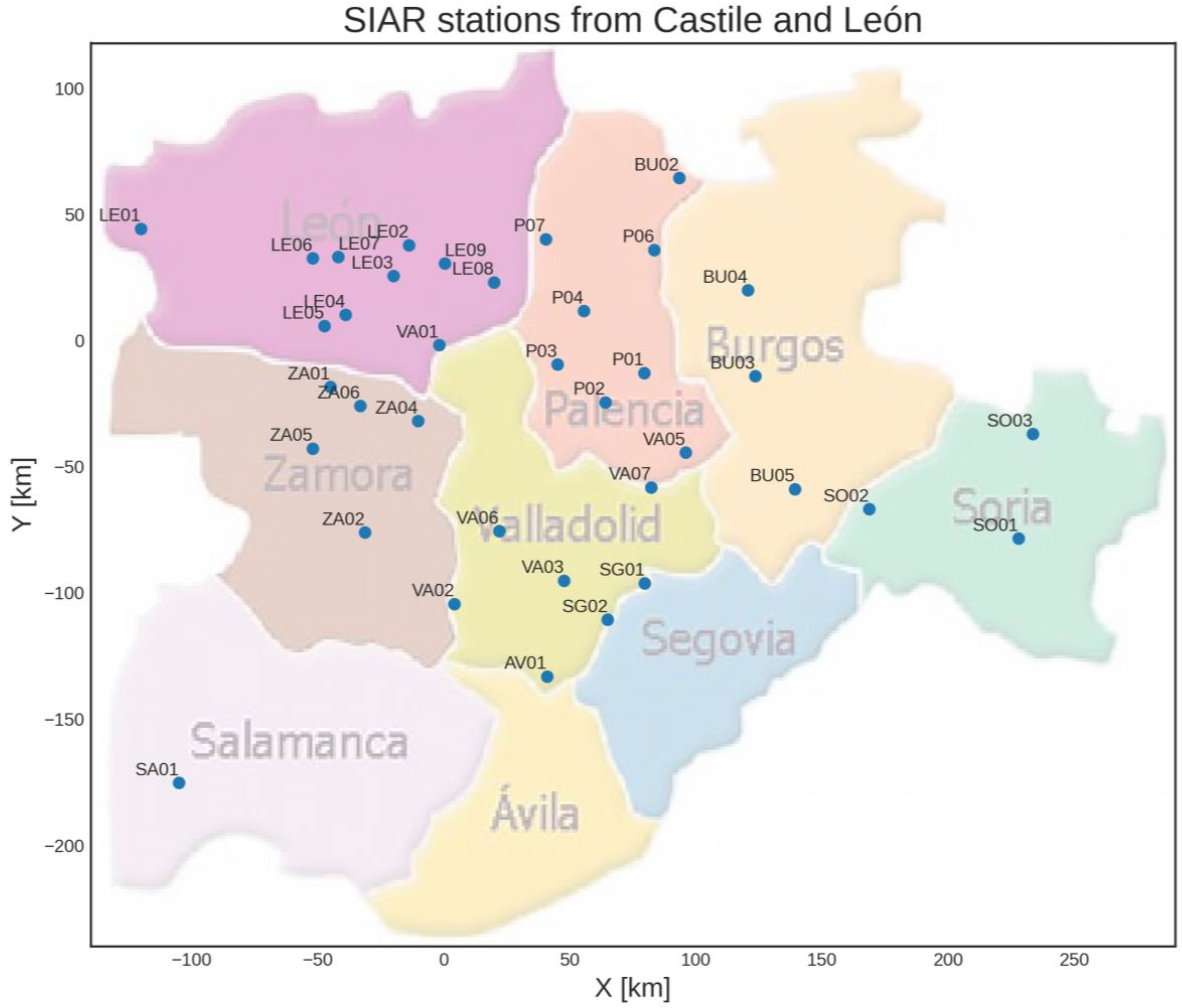
  • In its spatial representation, as it contains data from 37 stations that allow for a regional-level analysis (it covers a land area of approximately 94,226 km2).
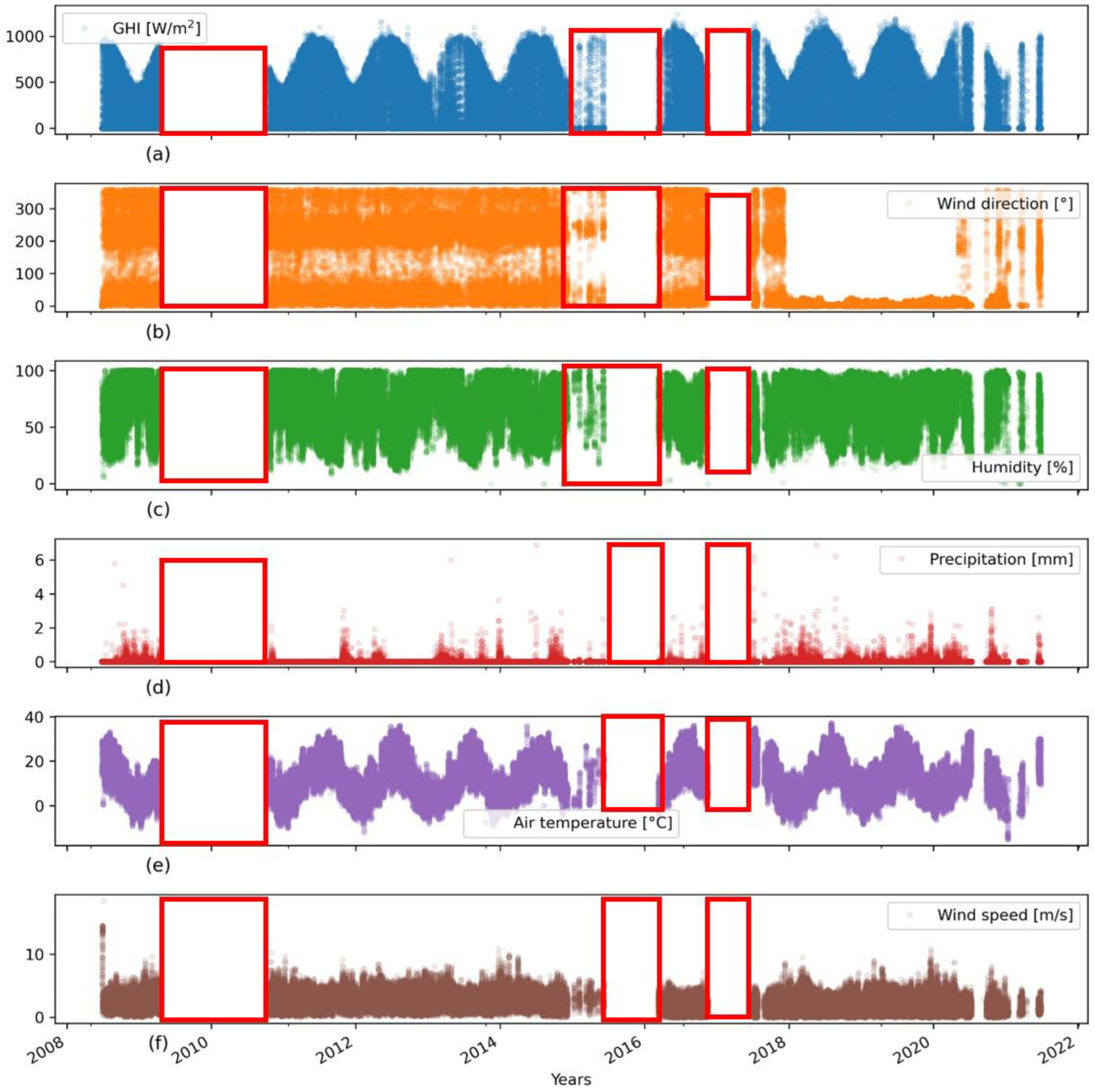
  • It contains meteorological variables that enable the analysis of correlation and the use of explanatory variables in the models to study their influence on performance.
  • Its publication allows other researchers to train their forecasting model implementations, without reapplying data cleaning and quality control procedures.
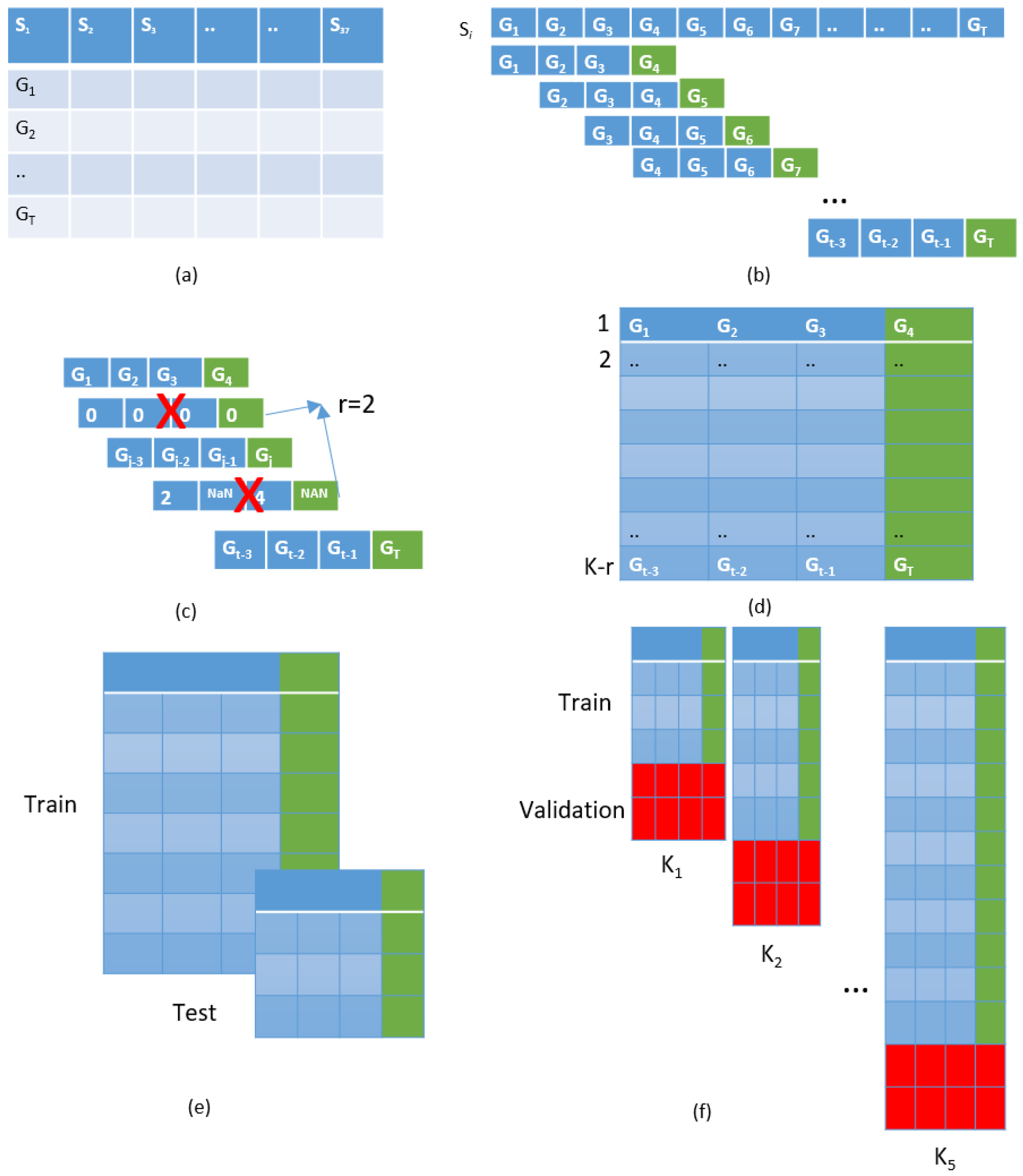
  • It can be used with emerging trends based on deep machine learning for solar irradiance forecasting and serve as a benchmark dataset where comparisons can be established between novel implementation models tested on the same data (as a train-data data split procedure is also proposed).
The remainder of the paper is organized as follows. Section 2, the process of obtaining, transforming, and quality control performed over the data is described. Section 3 presents a set of baseline models; Section 4 explains in detail the experiments carried out on the dataset as well as the analysis of the results. The manuscript ends with the conclusion section.

2. Data

In this section, we review the process of obtaining the dataset, starting with Section 2.1, where the methodology used to obtain the dataset is described. Section 2.2 shows the quality control carried out, Section 2.3 describes the dataset obtained, while Section 2.4 provides a brief description of ERA5, a public dataset used for comparison reasons.

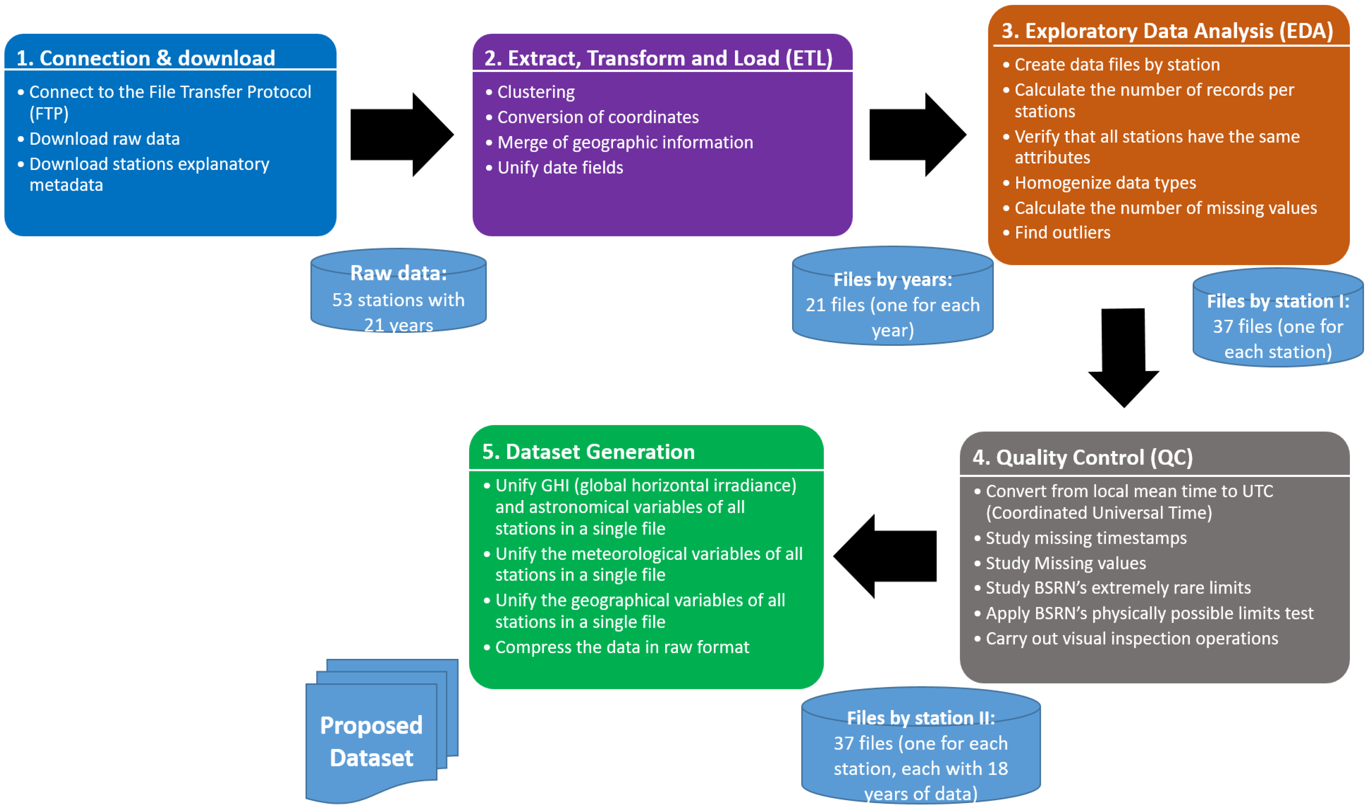
2.1. Procedure Applied for the Dataset Creation

For the dataset generation process, we applied the methodology illustrated in Figure 1. Briefly, we began by downloading all the available data offered by ITACyL, using a File Transfer Protocol (FTP) provided by the public agency. The data was then transformed using ETL (Extract, Transform, and Load) tools. Afterwards, we carried out an exploratory data analysis. The subsequent step was to perform a quality control (QC) of the data. In the end, the files were created for the proposed CyL-GHI dataset.
A detailed description of this methodology is presented below, where each of the steps involved in the process of obtaining the CyL-GHI dataset will be explained.

2.1.1. Raw Data

We started by downloading the 21-year hourly data from the 53 stations located in the Spanish autonomous community of Castile and León using the FTP service [32] provided by the ITACyL to generate the raw data. Figure 2 shows the spatial distribution of the stations forming the raw data within the Castile and León region. As can be found in Figure 2, the region has stations spread over its nine provinces, although the representation is denser towards the centre of the region.
The raw data downloaded from the FTP is pre-separated according to the following classification: hourly data, daily data, and monthly data—hourly and daily data being collected from 1 January 2001, to the present and monthly data being collected from 1 January 2019, onwards. The hourly data are disaggregated into folders named with the name of the year it contains; each folder containing a zip file for each day of the year. These files, in turn, store a csv file with the data collected for the day. The observations are captured with a frequency of 30 min.
The generic notation used to name the raw files is “20010101_RedClimaITACyL_Horario.csv”. In this mentioned formulation, “20010101” represents the year, month, and day; “RedClimaITACyL” represents the name of the network (ITACyL references the Agroclimatic Technological Institute of Castile and León); and “Horario” represents time granularity for data to be stored, while the “.csv” represents the file extension. Each raw file from every station illustrated in Figure 2 contains the variables described in Table 1.
The description of the equipment used to acquire the measurements at station-level is presented in Table 2. In Table 2, for each of the meteorological variables, the measurement ranges, the accuracy of the sensor, the measurement unit and the instrument used in the measurement is specified. The information regarding the data capturing instruments was compiled from the information provided by the ITACyL. According to its productor, as part of the SIAR network, all stations must undergo preventive maintenance every six months and annual calibration of the measuring sensors [33].

2.1.2. Extract, Transform and Load

In order to unify all the information in a single csv file, ETL tools were used to (1) group the zip files of the days in a csv file for each year; (2) convert of coordinates and spatial reference system (European Datum 1950 UTM projection Huso 30 to Geographic Coordinates European Terrestrial Reference System 1989); (3) merge the information related to the locations of the stations ( X and Y coordinates and height); and (4) unify the date and time fields into a single field with the format (yyyy-MM-dd HH:mm:ss).
The FTP service also provided a csv file consisting of descriptive information regarding the stations, namely, the fields “IDPROVINCE”, “IDSTATION”, “SHORT NAME”, “NAME”, “LENGTH (ED50 DDMMSS.SSS)”, and “LATITUDE (ED50 DDMMSS.SSS)”. The FTP service also provided the “HEIGHT”, “ X (UTM30N ED50)”, and “(UTM30N ED50)” variables that were used for assigning geographic data to the stations.

2.1.3. Exploratory Data Analysis

During the data exploration operation, it was found that only 37 of the 53 meteorological stations collected data since January 1st, 2001. The rest of the 16 stations were progressively incorporated into the network in the 2001–2012 period after which 53 stations have been maintained.
To have a global view of the stored data, all the variables of all stations for all years were plotted. Stations that had joined later were found to have long periods of missing data (as shown in Figure 3). The periods of absence observed varied from days to full months. This first inspection of the data also revealed the presence of outliers and errors. As part of the screening process, we calculated the number of records per station, verified that all stations had the same attributes (or characteristics), homogenized the data types, calculated the number of missing values, and validated the range of allowable values for each variable (considering the data published by ITACyL).
One of the most common identified problems was the absent data from the temperature, precipitations, and relative humidity variables (for example, that Station ZA02, located in Villaralbo, province of Zamora, had missing precipitation values since 2001). Another problem identified was that the data corresponding to the period 1st of January 2011 to 31st of January 2015 had the wrong year values in the time index of some of the stations.
The outcome of this exploratory process, a reduced dataset with 37 stations that contained complete data for the period from 1st of January 2002 to 31st of December 2019 was obtained, where the outliers values found were labelled with the data type NaN (Not a Number). Figure 4 shows the spatial representation of the 37 stations selected to be part of the CyL-GHI dataset. In this dataset, the spatial distribution is concentrated towards the centre of the region, and, apart from stations LE01 (Spanish: Carracedelo) and SA01 (Spanish: Ciudad Rodrigo) from the provinces of León and Salamanca), all the other stations are located within a 70 to 100 km range of each other.

2.2. Quality Control of Dataset

The quality control performed on the data is an important step in the creation of a dataset. There are different controls to be performed and, even within the experts in the field, types of controls differ between works [34], as shown below:
The “BSRN Global Network recommended QC tests, v2.0” [35] (BSRN stands for Baseline Surface Radiation Network) are considered amongst the most recognised. Wilbert et al. [34] proposed eight quality checks on the basis of the most commonly used in the literature. The quality checks are named (1) the missing timestamps; (2) the missing values; applying (3) the K-Tests; (4) the BSRN’s closure tests; (5) the BSRN’s extremely rare limits test [35]; (6) the BSRN’s physically possible limits test [35]; (7) the tracker-off test; and (8) carrying out a visual inspection. Of the eight quality controls proposed by Wilbert et al., the following five will be used in our analysis: (1)-missing timestamps; (2)-missing values; (4)-BSRN’s extremely rare limits test [35]; (5)-BSRN’s physically possible limits test; and (8)-visual inspection.

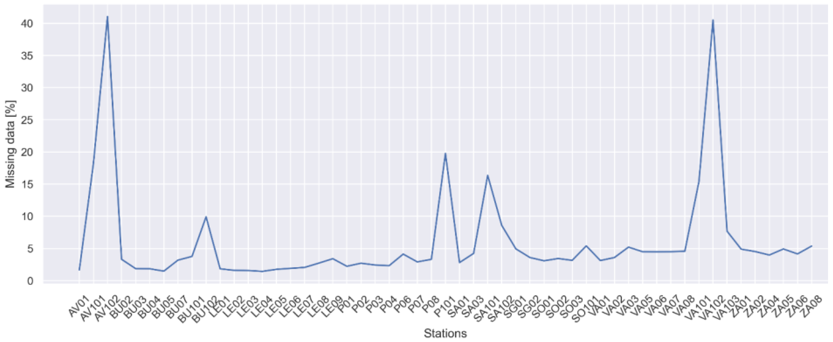
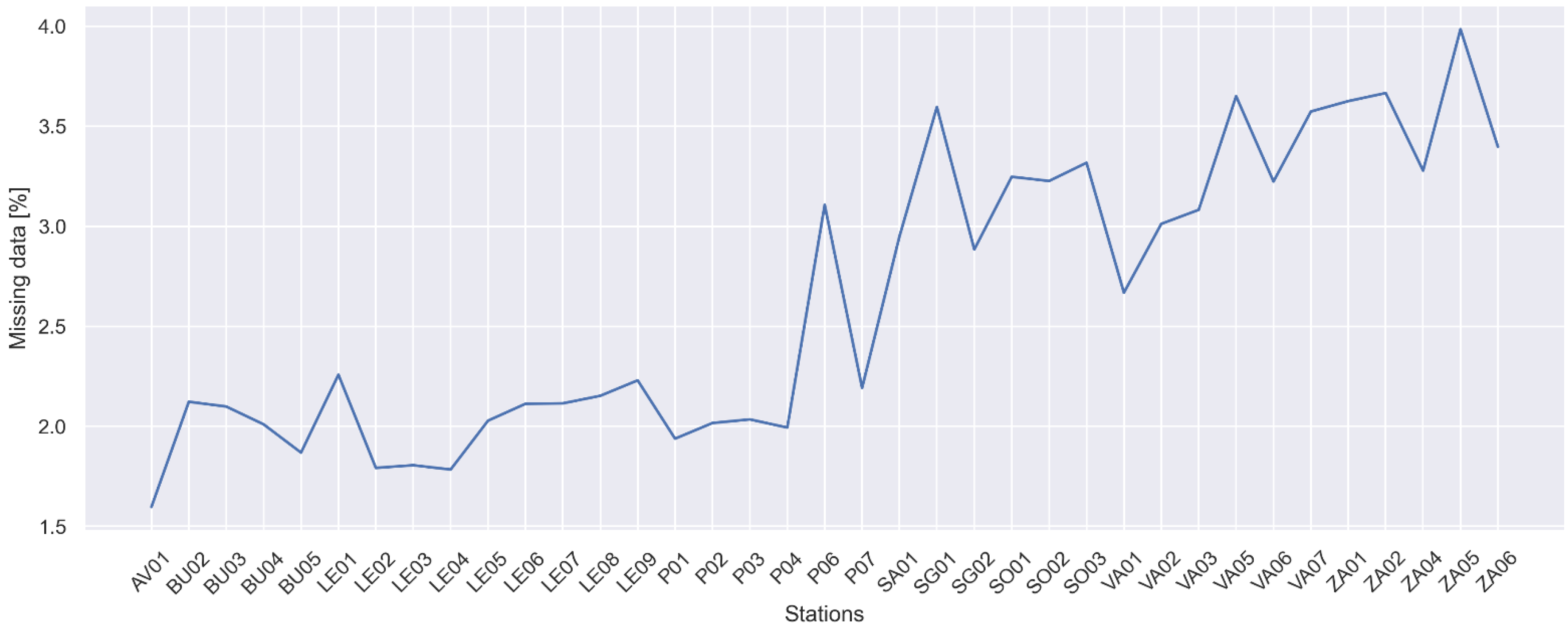
2.2.1. Missing Timestamps

For the quality control of a time series, its timestamps are essential, so the following had to be considered. Each station in the SIAR network of Castile and León has its own local mean solar time, corresponding to the meridian on which it is located. Before applying any control on the data, it was necessary to correct this issue by converting the data to the Universal Time Coordinated (UTC) format. The conversion was performed for each of the stations considering their longitude to correct the time error in their timestamps.
Furthermore, when collecting the data, there may be missing timestamps in the time series caused by failures of the equipment that performs the storage. In order to identify these gaps, an analysis of the time indexes was carried out, and, in cases where it was found that they were not complete, the time indexes were completed with the expected timestamps, and the corresponding series values were filled in with NaN values.

2.2.2. Missing Values

The presence of missing values can have several causes. Missing data may be due to the fact that values were not recorded for a specific time period because of inconsistency in the data acquisition equipment. Another possible cause is that, for a particular station or variable, one of the measurement equipment was not available (e.g., Station ZA02 located in Villaralbo, province of Zamora, is missing the values of the precipitation variable for the entire year of 2001, while station AV01, located in Nava de Arévalo, province of Avila, has hourly timestamps for the month of January 2001, and after 6th of February 2001, it starts delivering data with a granularity of 30 min).
An analysis was conducted for each of the stations in the raw data. As shown in Figure 5, there are stations that reach 40% data loss in the raw data. However, stations with high percentages of missing data were already left out of the final dataset in the first steps of the application of the methodology and are not presented in the CyL-GHI dataset.
The mean percentage of missing values in the CyL-GHI dataset is 2.64% (ranging from minimum 1.60% at the AV01 station to maximum 3.98% at the ZA05 station). It is important to note that missing values occurrence percentages are below 4% in all the stations that compose the CyL-GHI dataset, as shown in Figure 6.
The missing values in the CyL-GHI dataset were completed with NaN values to maintain the completeness of the time series time index (as having a complete time index is important in the pre-processing step of the dataset to obtain the input data structure for machine learning algorithms). After obtaining the time windows, it is possible to eliminate NaN values without losing the sequence necessary to contemplate past observations for prediction.

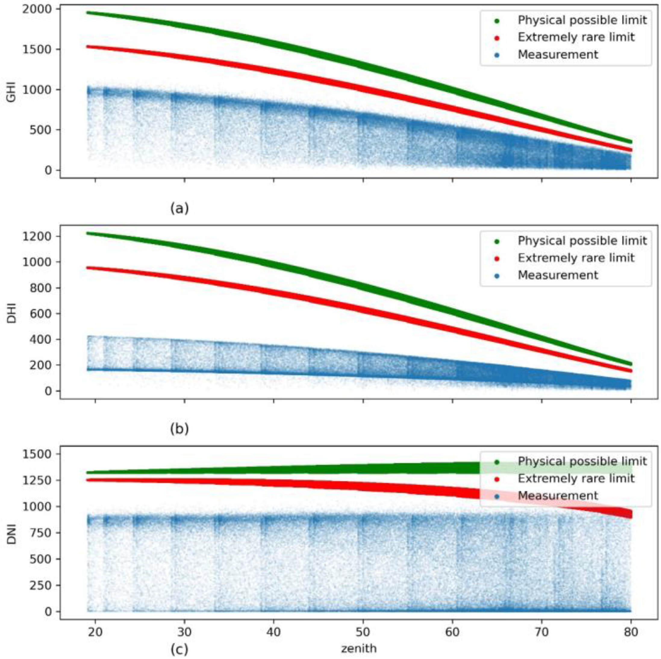
2.2.3. BSRN’s Limits Test

In this step, the limit set for the global horizontal irradiance was evaluated by calculating the irradiance value against extremely rare limits with Equation (1), and against physical possible limits with Equation (2) as follows.
4     G H I     1.5   ×   E T N   ×   c o s 1.2 ( S Z A ) + 100
2     G H I     1.2   ×   E T N   ×   c o s 1.2 ( S Z A ) + 50
In Equations (1) and (2), E T N represents the Extra-Terrestrial irradiance at Normal incidence, and S Z A represents the solar zenith angle. The astronomical variables required for the irradiance analysis were retrieved from the “Solar Geometry 2” [36] library, and the process calculates the astronomical information of each station considering the coordinates, height, period, and desired time resolution of the data. The mentioned library returned a file with universal Julian date (day), year, month of the year, day of the month, hour of the day (decimal hour), day of the year, topocentric declination (radian), topocentric hour angle (radian), topocentric Sun elevation angle without refraction correction (radian), topocentric Sun azimuth angle Eastward from North (radian), and Sun-Earth Radius (ua).
The data obtained with the above-mentioned library had to be processed to obtain new variables and to match the format in some cases. First, the fields referring to time were unified into a single field by transforming the decimal time to the “ h h : m m : s s ” format. Next, the sun elevation angle was used to calculate the solar zenith angle and the variable ETN. In the end, the variables Top of Atmosphere Radiation (toa), solar elevation angle, and azimuth angle were kept as part of the final dataset.
Graphical representations of Extremely rare limits and Physical possible limits, proposed by [37], were created for all the 37 stations from the CyL-GHI dataset for the GHI, Direct Normal Irradiance (DNI), and Diffuse Horizontal Irradiance (DHI) variables (an example is shown in Figure 7 for the station BU04 in the province of Burgos). The DNI and DHI variables were calculated from the GHI values using the pvlib library [38], as they were not part of our initial raw data.

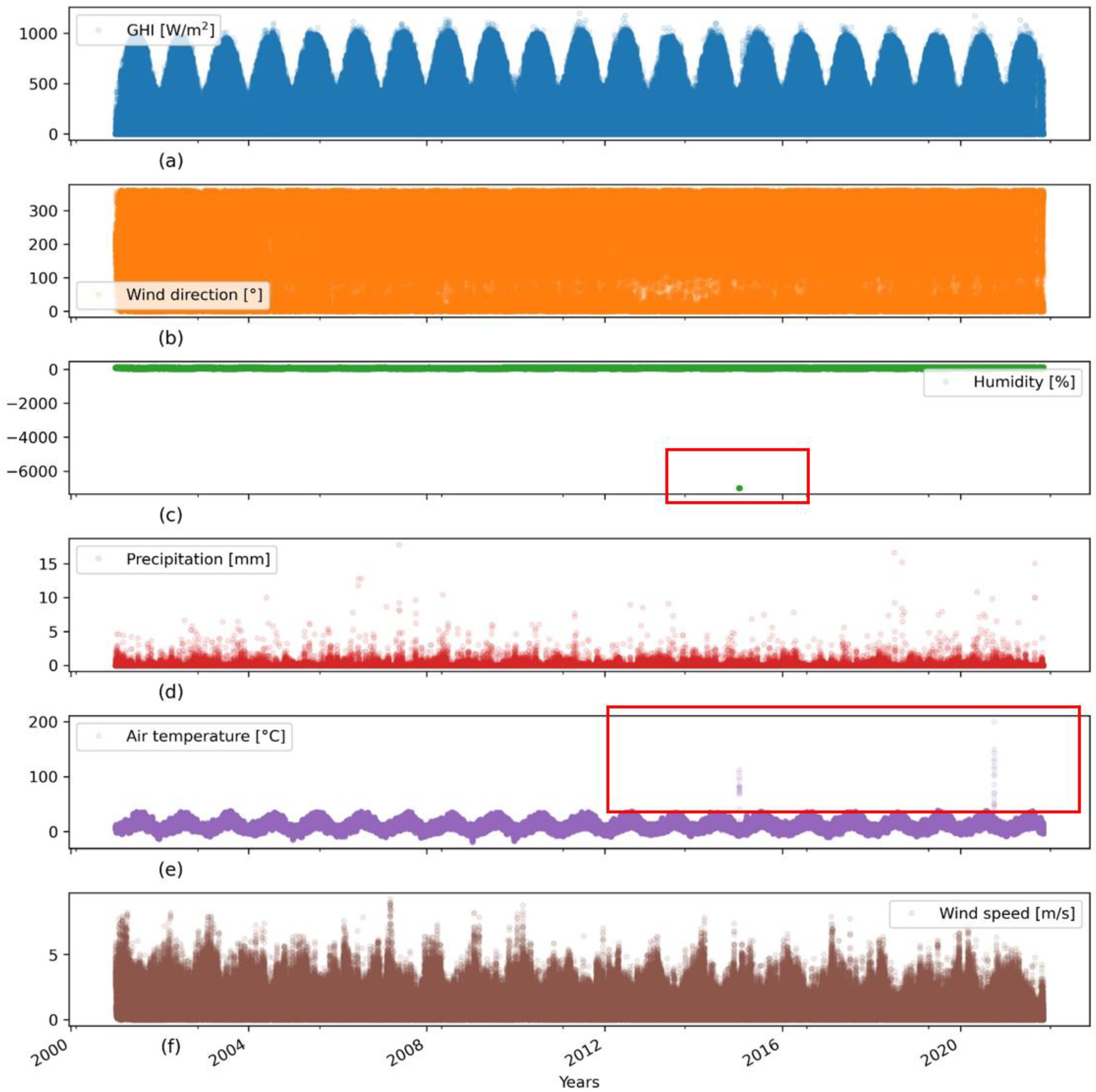
2.2.4. Visual Inspection

In datasets where, large time windows and stations distributed over large areas are considered at the same time, a visual inspection of the measurements is complex. For this reason, we applied this operation in the data exploration stage to visualise the GHI and the meteorological variables for all years for each of the stations, and even carried out specific analysis of individual stations or years when needed.
By carrying out this operation in each station for the whole considered period, we managed to detect the presence of extreme outliers (as shown in Figure 8 for the case of the relative humidity and air temperature variables for the station BU03, located in Lerma, in the province of Burgos) or to find missing data at month level (Figure 9). Automated error-finding processes complemented this operation, and, after the search process, the errors found were analysed, and actions were taken to correct them.

2.3. Dataset Description

CyL-GHI data is based on the raw data provided by the public agency Agroclimatic Technological Institute of Castile and León (ITACyL), where refinement operations have been applied. The raw data contains 21 files grouped into folders that were downloaded directly from a service provided by ITACyL [31]. The original raw data contained information from a period of 21 years (January 1st, 2001, to November 11, 2021) for the 53 stations found in the considered region.
The CyL-GHI dataset is provided in three csv (Comma Separated Values) files (“CyL_GHI_ast.csv”, “CyL_meteo.csv”, and “CyL_geo.csv”) and two zip (compressed file format) files (“CyL_by_stations.zip” and “CyL_raw.zip”), and can be downloaded from the Zenodo repository [39] under a CC-BY-SA-NC license.
CyL-GHI contains records from 1st of January 2002 to 31st of December 2019, with a time granularity of 30 min, from 37 stations located in Castile and León.
Table 3 presents the name of files found in the Zenodo repository [39] and a brief description of its data and variables. It is important to note that, when training forecasting models, the first 17 years (data from 1st of January 2002 to 31st of December 2018) should be used for training, while data corresponding to the last year of the CyL-GHI dataset (the period from 1st of January 2019 to 31st of December 2019) should be used to test the performance of the forecasting implementation. The forecasting model did not have access to the testing data during training. This requirement with respect to the partitioning of the data in order to be able to make fair comparisons between models based on the use of the CyL-GHI dataset.

2.4. ERA5

ERA5 is the fifth reanalysis data set from the European Centre for Medium-range Weather Forecasts (ECMWF) [40]. According to its producer, the ERA5 data published covers the period starting from 1950 to present and new data continuously added in near-real time. The Global Horizontal Irradiance variable provided by ERA5 as “Mean surface downward short-wave radiation flux” features a spatial resolution of 31 km and a temporal resolution of one hour. For this study, GHI data corresponding to our studied region was downloaded from the official repository [41] from 1st of January 2002 to 31 December 2019. It is important to mention that resampling to a frequency of 30 min had to be carried out to align the temporal resolution of ERA5 to our data. The resulting data was used to compare the performance of the optimised baseline models with the ERA5 GHI data (in Section 4).

3. Baseline Models

Next, three widely used models were trained on the CyL-GHI dataset to be used as a baseline to allow future comparison with more complex models, namely, the Persistence and Linear models, a tree-based model, together with a support vector model. In particular, Random forest (RF) and Support Vector Regression (SVR) models were chosen for the study because they have been used with good results in solar forecast [42,43,44,45]. In 2017, Voyant et al. [46] performed an analysis of machine learning models that included them and predicted their future importance in the field of solar forecast. In addition, as more complex models have appeared, these models have been kept as a baseline to evaluate the effectiveness of these new models. The RF and SVR models have been used as baselines in multiple studies either independently (RF [47,48,49,50], SVR [51,52,53,54,55]) or both in the same study [56,57].
(1) The Persistence model is a naïve model that is widely used in the literature and delivers acceptable results for short prediction horizons. It consists of using the previous observation as the input of the next prediction. Equation (3) defines the model, where G represents the global horizontal irradiance.
G t = G t 1  
(2) The Linear Regression model (LR) defined in Equation (4) assumes that the value to be predicted is a consequence of a linear combination of previous observations.
G t = l a l G ( t l ) + b
In Equation (4),   l represents the lags (past observations) used for the prediction; a l   represents regression coefficients, and   b   is the bias term.
(3) The RF model [58] consists of a generating multitude of classifiers structured as trees. In regression tasks, a RF model will return the average of the individual trees predictions as the final prediction.
(4) SVR algorithm [59] applied in regression tasks. During training, SVR translates the data from the existing input space into the feature space and will model an optimal regression function that is capable of mapping the data expressed in a high-dimensional space, while achieving the minimum error. However, it is important to mention that, when considering a large number of characteristics for training, the computational cost increases exponentially.
The three baseline models use different approaches to process the predictors. The results will let other researchers to preview the behaviour of the dataset with different machine learning models.

4. Experiments, Results and Discussion

To carry out the experiments, the initial phase is to transform the data into the data structure expected by the machine learning models. For this purpose, a set of steps had to be performed, which are described graphically in Figure 10.
As shown in Figure 10a, we start from the initial CyL-GHI (CyL_GHI_ast.csv) dataset. The initial dataset has a GHI time series represented by S i for each of the 37 stations. Each time series, S i , corresponding to the columns of the matrix, illustrated in Figure 10a, is transformed using the window sliding method shown in Figure 10b. This method creates the input and output of the model, where the input is formed by previous GHI observations, and the output is the GHI value for the time horizon to be predicted.
The next step (presented in Figure 10c) is based on the solar elevation angle of 5° and uses data where the night-time hours data and NaN values data are eliminated. A matrix containing the concatenation of all valid windows for the prediction is formed after the reduction in step (c) (as presented in Figure 10d). The matrix is divided into train and testing sets (Figure 10e). For training, data from the first 17 years (from 1st of January 2002 to 31st of December 2018) was used, while, for evaluating the performance on unseen data, the last year of the dataset (the period from 1st of January 2019 to 31st of December 2019) was to be used.
To optimize the results, a search for the best parameters for each model and time series was carried out and a five-fold cross validation evaluation was performed (as presented in Figure 10f). The cross-validation operation is only performed on the train set (obtained in step (e)), and it is important to properly partition the time series data according to the time index (since future data must not be used for training).
The selection of the number of past observations used as input to the model varies depending on several factors such as the temporal resolution of the data, the prediction model chosen, among others. There are authors who used two to three past observations [60,61] and others who used a range of values [62,63] to evaluate which best fit the configuration of their model. In this study, the past observations corresponding to the last 24 h period was taken as the input, and the outputted, predicted value corresponds to one instance of time forward (the forecast horizon would be a single step, i.e., for the future thirty min). This selection was made after an autocorrelation analysis and exploration of the best performing combination.
The models were implemented in the Python programming language using the scikit-learn library [64]. The values of the explored parameters for the RF and SVR models are shown in Table 4.
The metrics considered in the evaluation of the performance of the trained models on unseen data are, Mean Absolute Error ( M A E ), Root Mean Squared Error ( R M S E ), and Forecast Skill ( F S ), defined by Equations (5)–(7), respectively.
M A E = i = 1 n | ( y i y ^ i ) | n
R M S E = 1 n i = 1 n ( y i y ^ i ) 2
F S = 1 R M S E m o d e l R M S E p e r s i s t e n c e
The results of evaluating the 37 stations on unseen data for each of the models offered as baseline values of the machine learning implementations on the CyL-GHI dataset (CyL_GHI_ast.csv) is shown in Table 5.
In average values, the Persistence achieved a RMSE of 90.69 W/m2, while the ERA5 obtained a RMSE of 94.08 W/m2. It is observed that the regression models provide higher performance values (within the range of 64.44 W/m2 to 69.05 W/m2) and achieve an improvement of 30 W/m2 in average when compared to the Persistence and ERA5.
According to the mean RMSE and FS metrics, RF is the model with the highest prediction capacity. SVR forecast skill is the lowest with respect to other models trained (this may be caused by the form the models perform the regularization). The LR and SVR models have an average forecast skill with respect to all stations of 25.12% and 24.07%, respectively, and there is a reduced difference between them. The RF model represents an average improvement of 5.0% with respect to the LR and SVR models.
In another experiment, of RF, we also explored the influence of different combinations of parameter values on the predictive capacity of the model. The following three training scenarios were considered: (1) the model was implemented with the default parameters, (2) a parameter optimisation was performed for each of the stations, and (3) the exogenous variables were included (lags of neighbours and solar elevation and zenith angles). The average results of the evaluation on unseen data for each station of CyL-GHI are presented as boxplots in Figure 11.
Figure 11 shows the difference between the averages in which the performance values oscillate, from 28% for the first scenario evaluated to 33% for the third scenario evaluated. The inclusion of previous observations from neighbours delivered a 3% improvement between Scenarios 2 and 3, which indicates the assumption that the dataset used in a spatio-temporal analysis (i.e., introducing information from neighbours) can achieve improvements in decreasing the forecasting error at the target station. The results illustrated in Figure 11 also show that it is possible to achieve an increase in the model skill as a function of the refinement of the parameters and the increase in the input variables.

5. Conclusions

In this paper, the methodology applied to introduce a large-scale, public, and irradiance dataset, CyL-GHI, has been presented. The methodology proposed for the obtained dataset from raw data has also been explained and involved several operations such as downloading the data, pre-processing, and applying quality control procedures, and could be reapplied to other similar data generation tasks. It should also be noted that, as part of the processing of the dataset, the transformation from Local Mean Time to UTC was performed, and astronomical variables calculated based on the geographic data of the stations were also included. CyL-GHI can result important for research purposes in the field of solar forecasting.
In addition, the performance metrics of four baseline models on unseen data have been provided as benchmark performance values for comparisons with future implementations, as well as for the analysis of the results obtained on the proposed dataset. For training, data from the first 18 years of the dataset was used for training (from 1st of January 2002 to 31st of December 2018), while the data from the last year (1st of January 2019 to 31st of December 2019) was used for testing the performance of the trained models. Furthermore, the ERA5 values corresponding to the studied area were analysed and compared with performance values delivered by the trained models.
Tests performed with the Random Forest model on the CyL-GHI dataset indicate that the forecast error of a model can be reduced by adding variables from its neighbouring stations. As future works, it is expected to use the dataset with models of emerging trends such as deep learning in data science that exploit the spatio-temporal characteristics of the irradiance data.

Author Contributions

Conceptualisation, L.B.C. and M.Á.M.C.; methodology, L.B.C. and M.Á.M.C.; software, L.B.C.; validation, L.B.C., M.Á.M.C. and C.-I.C.; investigation, L.B.C.; resources, M.Á.M.C., C.-I.C. and R.A.; data curation, L.B.C.; writing—original draft preparation, L.B.C.; writing—review and editing, L.B.C., M.Á.M.C., C.-I.C. and R.A.; visualisation, L.B.C.; supervision, M.Á.M.C. and C.-I.C. All authors have read and agreed to the published version of the manuscript.

Funding

This work was supported by “Feature extraction and renewable energy estimation (RP2212570003)” Universidad Politécnica de Madrid’s own project.

Institutional Review Board Statement

Not applicable.

Informed Consent Statement

Not applicable.

Data Availability Statement

CyL-GHI data available at https://doi.org/10.5281/zenodo.7404167.

Acknowledgments

The authors would like to thank Rodrigo Amaro e Silva for his help in the process of creating up the dataset and in the initial phases of the research.

Conflicts of Interest

The authors declare no conflict of interest.

References

  1. Yang, D. A guideline to solar forecasting research practice: Reproducible, operational, probabilistic or physically-based, ensemble, and skill (ROPES). J. Renew. Sustain. Energy 2019, 11, 022701. [Google Scholar] [CrossRef]
  2. Camal, S.; Kariniotakis, G.; Sossan, F.; Libois, Q.; Legrand, R.; Raynaud, L.; Lange, M.; Mehrens, A.; Pinson, P.; Pierrot, A.; et al. Smart4RES: Next generation solutions for renewable energy forecasting and applications with focus on distribution grids. In Proceedings of the CIRED 2021—The 26th International Conference and Exhibition on Electricity Distribution, Online, 20–23 September 2021; pp. 2899–2903. [Google Scholar] [CrossRef]
  3. Yang, D. SolarData: An R package for easy access of publicly available solar datasets. Sol. Energy 2018, 171, A3–A12. [Google Scholar] [CrossRef]
  4. Feng, C.; Yang, D.; Hodge, B.-M.; Zhang, J. OpenSolar: Promoting the openness and accessibility of diverse public solar datasets. Sol. Energy 2019, 188, 1369–1379. [Google Scholar] [CrossRef]
  5. Peterson, J.; Vignola, F. Structure of a comprehensive solar radiation dataset. Sol. Energy 2020, 211, 366–374. [Google Scholar] [CrossRef]
  6. Yang, D.; Wang, W.; Hong, T. A historical weather forecast dataset from the European Centre for Medium-Range Weather Forecasts (ECMWF) for energy forecasting. Sol. Energy 2022, 232, 263–274. [Google Scholar] [CrossRef]
  7. Dua, D.; Graff, C. UCI Machine Learning Repository; University of California, School of Information and Computer Science: Irvine, CA, USA, 2017; [Online]; Available online: http://archive.ics.uci.edu/ml (accessed on 1 December 2022).
  8. Goldbloom, A. Kaggle. 2010. Available online: https://www.kaggle.com/datasets (accessed on 1 December 2022).
  9. Leach-Murray, S. The Linked Open Data Cloud. Tech. Serv. Q. 2021, 38, 193–194. [Google Scholar] [CrossRef]
  10. Bright, J.M.; Killinger, S.; Engerer, N.A. Data article: Distributed PV power data for three cities in Australia. J. Renew. Sustain. Energy 2019, 11, 035504. [Google Scholar] [CrossRef]
  11. Driemel, A.; Augustine, J.; Behrens, K.; Colle, S.; Cox, C.; Cuevas-Agulló, E.; Denn, F.M.; Duprat, T.; Fukuda, M.; Grobe, H.; et al. Baseline Surface Radiation Network (BSRN): Structure and data description (1992–2017). Earth Syst. Sci. Data 2018, 10, 1491–1501. [Google Scholar] [CrossRef] [Green Version]
  12. Haysom, J.E.; McVey-White, P.; De La Salle, L.; Hinzer, K.; Schriemer, H. Multi-year ground-based irradiance dataset in a northern urban climate. In Proceedings of the 2017 IEEE 44th Photovoltaic Specialist Conference, PVSC 2017, Washington, DC, USA, 25–30 June 2017; pp. 796–801. [Google Scholar] [CrossRef]
  13. Pedro, H.T.C.; Larson, D.P.; Coimbra, C.F.M. A comprehensive dataset for the accelerated development and benchmarking of solar forecasting methods. J. Renew. Sustain. Energy 2019, 11, 036102. [Google Scholar] [CrossRef] [Green Version]
  14. Terrén-Serrano, G.; Bashir, A.; Estrada, T.; Martínez-Ramón, M. Girasol, a sky imaging and global solar irradiance dataset. Data Brief 2021, 35, 106914. [Google Scholar] [CrossRef]
  15. Charabi, Y.; Gastli, A.; Al-Yahyai, S. Production of solar radiation bankable datasets from high-resolution solar irradiance derived with dynamical downscaling Numerical Weather prediction model. Energy Rep. 2016, 2, 67–73. [Google Scholar] [CrossRef] [Green Version]
  16. Qin, W.; Wang, L.; Gueymard, C.A.; Bilal, M.; Lin, A.; Wei, J.; Zhang, M.; Yang, X. Constructing a gridded direct normal irradiance dataset in China during 1981–2014. Renew. Sustain. Energy Rev. 2020, 131, 110004. [Google Scholar] [CrossRef]
  17. Williamson, S.; Businger, S.; Matthews, D. Development of a solar irradiance dataset for Oahu, Hawaii. Renew. Energy 2018, 128, 432–443. [Google Scholar] [CrossRef]
  18. Simeunovic, J.; Schubnel, B.; Alet, P.-J.; Carrillo, R.E. Spatio-Temporal Graph Neural Networks for Multi-Site PV Power Forecasting. IEEE Trans. Sustain. Energy 2022, 13, 1210–1220. [Google Scholar] [CrossRef]
  19. Cesar, L.B.; e Silva, R.A.; Callejo, M.M.; Cira, C.-I. Review on Spatio-Temporal Solar Forecasting Methods Driven by in Situ Measurements or Their Combination with Satellite and Numerical Weather Prediction (NWP) Estimates. Energies 2022, 15, 4341. [Google Scholar] [CrossRef]
  20. e Silva, R.A.; Brito, M. Spatio-temporal PV forecasting sensitivity to modules’ tilt and orientation. Appl. Energy 2019, 255, 113807. [Google Scholar] [CrossRef]
  21. Khodayar, M.; Mohammadi, S.; Khodayar, M.E.; Wang, J.; Liu, G. Convolutional Graph Autoencoder: A Generative Deep Neural Network for Probabilistic Spatio-Temporal Solar Irradiance Forecasting. IEEE Trans. Sustain. Energy 2019, 11, 571–583. [Google Scholar] [CrossRef]
  22. Yu, Y.; Hu, G. Short-term solar irradiance prediction based on spatiotemporal graph convolutional recurrent neural network. J. Renew. Sustain. Energy 2022, 14, 053702. [Google Scholar] [CrossRef]
  23. Karimi, A.M.; Wu, Y.; Koyuturk, M.; French, R.H. Spatiotemporal Graph Neural Network for Performance Prediction of Photovoltaic Power Systems. In Proceedings of the AAAI Conference on Artificial Intelligence, Online, 2–9 February 2021; Volume 35, pp. 15323–15330, [Online]. Available online: https://ojs.aaai.org/index.php/AAAI/article/view/17799 (accessed on 15 January 2022).
  24. Agoua, X.; Girard, R.; Kariniotakis, G. Photovoltaic Power Forecasting: Assessment of the Impact of Multiple Sources of Spatio-Temporal Data on Forecast Accuracy. Energies 2021, 14, 1432. [Google Scholar] [CrossRef]
  25. AEMET. Agencia Estatal de Meteorología. Available online: http://www.aemet.es/es/portada (accessed on 22 February 2022).
  26. SIAR. Sistema de Información Agroclimática para el Regadío. Available online: https://eportal.mapa.gob.es/websiar/Inicio.aspx (accessed on 12 January 2022).
  27. Rodríguez-Amigo, M.; Díez-Mediavilla, M.; González-Peña, D.; Pérez-Burgos, A.; Alonso-Tristán, C. Mathematical interpolation methods for spatial estimation of global horizontal irradiation in Castilla-León, Spain: A case study. Sol. Energy 2017, 151, 14–21. [Google Scholar] [CrossRef]
  28. Eschenbach, A.; Yepes, G.; Tenllado, C.; Gomez-Perez, J.I.; Pinuel, L.; Zarzalejo, L.F.; Wilbert, S. Spatio-Temporal Resolution of Irradiance Samples in Machine Learning Approaches for Irradiance Forecasting. IEEE Access 2020, 8, 51518–51531. [Google Scholar] [CrossRef]
  29. Gutierrez-Corea, F.-V.; Manso-Callejo, M.-A.; Moreno-Regidor, M.-P.; Manrique-Sancho, M.-T. Forecasting short-term solar irradiance based on artificial neural networks and data from neighboring meteorological stations. Sol. Energy 2016, 134, 119–131. [Google Scholar] [CrossRef]
  30. Urraca, R.; Antonanzas, J.; Sanz-Garcia, A.; Martinez-De-Pison, F.J. Analysis of Spanish Radiometric Networks with the Novel Bias-Based Quality Control (BQC) Method. Sensors 2019, 19, 2483. [Google Scholar] [CrossRef] [Green Version]
  31. ITACYL. Instituto Tecnológico Agrario de Castilla y León. 2014. Available online: http://www.itacyl.es/opencms_wf/opencms/itacyl/quienes_somos/que_es_itacyl/index.html (accessed on 12 January 2022).
  32. ITACYL. Geoportal. 2015. Available online: ftp://ftp.itacyl.es (accessed on 10 November 2021).
  33. SIAR. Mantenimiento de las Estaciones del Siar. Available online: https://servicio.mapa.gob.es/es/desarrollo-rural/temas/gestion-sostenible-regadios/Mantenimiento%20de%20las%20estaciones_tcm30-82950.pdf (accessed on 15 January 2023).
  34. Forstinger, A.; Wilbert, S.; Kraas, B.; Peruchena, C.F.; Gueymard, C.A.; Collino, E.; Ruiz-Arias, J.A.; Martinez, J.P.; Saint-Drenan, Y.-M.; Ronzio, D.; et al. Expert Quality Control of Solar Radiation Ground Data Sets. In Proceedings of the ISES Solar World Congress, New Delhi, India, 25–29 October 2021. [Google Scholar]
  35. Long, N.; Dutton, G. BSRN Global Network Recommended QC Tests, V2.0, BSRN Technical Report. 2002. [Online]. Available online: https://bsrn.awi.de/fileadmin/user_upload/bsrn.awi.de/Publications/BSRN_recommended_QC_tests_V2.pdf (accessed on 24 June 2022).
  36. Blanc, P.; Wald, L. The SG2 algorithm for a fast and accurate computation of the position of the Sun for multi-decadal time period. Sol. Energy 2012, 86, 3072–3083. [Google Scholar] [CrossRef] [Green Version]
  37. Jensen, A.R.; Saint-Drenan, Y.-M. Solar Resource Assessment in Python. 2022. Available online: https://assessingsolar.org/intro.html (accessed on 16 November 2022).
  38. Holmgren, W.F.; Hansen, C.W.; Mikofski, M.A. Pvlib python: A python package for modeling solar energy systems. J. Open Source Softw. 2018, 3, 884. [Google Scholar] [CrossRef] [Green Version]
  39. Cesar, L.B.; Callejo, M.Á.M.; Cira, C.-I.; Garrido, R.P.A. CyL_GHI [Data Set]. Zenodo. 2022. [CrossRef]
  40. ECMWF. ERA5 Data Documentation; European Centre for Medium-Range Weather Forecast (ECMWF): Reading, UK, 2017; Available online: https://confluence.ecmwf.int/display/CKB/ERA5%3A+data+documentation (accessed on 14 February 2023).
  41. ECWMF. ERA5-Land Hourly Data from 1950 to Present. Available online: https://cds.climate.copernicus.eu/cdsapp#!/dataset/reanalysis-era5-land?tab=form (accessed on 14 February 2023).
  42. Babar, B.; Luppino, L.T.; Boström, T.; Anfinsen, S.N. Random forest regression for improved mapping of solar irradiance at high latitudes. Sol. Energy 2020, 198, 81–92. [Google Scholar] [CrossRef]
  43. Srivastava, R.; Tiwari, A.; Giri, V. Solar radiation forecasting using MARS, CART, M5, and random forest model: A case study for India. Heliyon 2019, 5, e02692. [Google Scholar] [CrossRef] [Green Version]
  44. Alfadda, A.; Adhikari, R.; Kuzlu, M.; Rahman, S. Hour-ahead solar PV power forecasting using SVR based approach. In Proceedings of the 2017 IEEE Power & Energy Society Innovative Smart Grid Technologies Conference (ISGT), Washington, DC, USA, 23–26 April 2017; pp. 1–5. [Google Scholar] [CrossRef]
  45. Silva, R.A.E.; da Silva, L.C.C.T.; Brito, M.C. Support vector regression for spatio-temporal PV forecasting PV variability The need for PV forecasting. In Proceedings of the 35th EUPVSEC 2018, Brussels, Belgium, 24–28 September 2018. [Google Scholar] [CrossRef]
  46. Voyant, C.; Notton, G.; Kalogirou, S.; Nivet, M.-L.; Paoli, C.; Motte, F.; Fouilloy, A. Machine learning methods for solar radiation forecasting: A review. Renew. Energy 2017, 105, 569–582. [Google Scholar] [CrossRef]
  47. Moncada, A.; Richardson, J.W.; Vega-Avila, R. Deep Learning to Forecast Solar Irradiance Using a Six-Month UTSA SkyImager Dataset. Energies 2018, 11, 1988. [Google Scholar] [CrossRef] [Green Version]
  48. Ghimire, S.; Deo, R.C.; Raj, N.; Mi, J. Deep Learning Neural Networks Trained with MODIS Satellite-Derived Predictors for Long-Term Global Solar Radiation Prediction. Energies 2019, 12, 2407. [Google Scholar] [CrossRef] [Green Version]
  49. Feng, C.; Zhang, J. SolarNet: A Deep Convolutional Neural Network for Solar Forecasting via Sky Images. In Proceedings of the 2020 IEEE Power & Energy Society Innovative Smart Grid Technologies Conference (ISGT), Washington, DC, USA, 17–20 February 2020; pp. 1–5. [Google Scholar] [CrossRef]
  50. Park, J.; Moon, J.; Jung, S.; Hwang, E. Multistep-Ahead Solar Radiation Forecasting Scheme Based on the Light Gradient Boosting Machine: A Case Study of Jeju Island. Remote Sens. 2020, 12, 2271. [Google Scholar] [CrossRef]
  51. Yang, T.; Li, B.; Xun, Q. LSTM-Attention-Embedding Model-Based Day-Ahead Prediction of Photovoltaic Power Output Using Bayesian Optimization. IEEE Access 2019, 7, 171471–171484. [Google Scholar] [CrossRef]
  52. Zhou, S.; Zhou, L.; Mao, M.; Xi, X. Transfer Learning for Photovoltaic Power Forecasting with Long Short-Term Memory Neural Network. In Proceedings of the 2020 IEEE International Conference on Big Data and Smart Computing (BigComp), Busan, Republic of Korea, 19–22 February 2020; pp. 125–132. [Google Scholar] [CrossRef]
  53. Simeunović, J.; Schubnel, B.; Alet, P.-J.; Carrillo, R.E.; Frossard, P. Interpretable temporal-spatial graph attention network for multi-site PV power forecasting. Appl. Energy 2022, 327, 120127. [Google Scholar] [CrossRef]
  54. Sodsong, N.; Yu, K.M.; Ouyang, W. Short-Term Solar PV Forecasting Using Gated Recurrent Unit with a Cascade Model. In Proceedings of the 2019 International Conference on Artificial Intelligence in Information and Communication (ICAIIC), Okinawa, Japan, 11–13 February 2019; pp. 292–297. [Google Scholar]
  55. Khodayar, M.; Liu, G.; Wang, J.; Kaynak, O.; Khodayar, M.E. Spatiotemporal Behind-the-Meter Load and PV Power Forecasting via Deep Graph Dictionary Learning. IEEE Trans. Neural Netw. Learn. Syst. 2021, 32, 4713–4727. [Google Scholar] [CrossRef] [PubMed]
  56. Aslam, M.; Lee, J.-M.; Kim, H.-S.; Lee, S.-J.; Hong, S. Deep Learning Models for Long-Term Solar Radiation Forecasting Considering Microgrid Installation: A Comparative Study. Energies 2019, 13, 147. [Google Scholar] [CrossRef] [Green Version]
  57. Jebli, I.; Belouadha, F.-Z.; Kabbaj, M.I.; Tilioua, A. Prediction of solar energy guided by pearson correlation using machine learning. Energy 2021, 224, 120109. [Google Scholar] [CrossRef]
  58. Breiman, L. Random Forests. Mach. Learn. 2001, 45, 5–32. [Google Scholar] [CrossRef] [Green Version]
  59. Cortes, C.; Vapnik, V. Support-vector networks. Mach. Learn. 1995, 20, 273–297. [Google Scholar] [CrossRef]
  60. Belaid, S.; Mellit, A.; Boualit, H.; Zaiani, M. Hourly global solar forecasting models based on a supervised machine learning algorithm and time series principle. Int. J. Ambient. Energy 2020, 43, 1707–1718. [Google Scholar] [CrossRef]
  61. Huang, C.; Wang, L.; Lai, L.L. Data-Driven Short-Term Solar Irradiance Forecasting Based on Information of Neighboring Sites. IEEE Trans. Ind. Electron. 2019, 66, 9918–9927. [Google Scholar] [CrossRef]
  62. Lazzaroni, M.; Ferrari, S.; Piuri, V.; Salman, A.; Cristaldi, L.; Faifer, M. Models for solar radiation prediction based on different measurement sites. Measurement 2015, 63, 346–363. [Google Scholar] [CrossRef]
  63. Huang, X.; Zhang, C.; Li, Q.; Tai, Y.; Gao, B.; Shi, J. A Comparison of Hour-Ahead Solar Irradiance Forecasting Models Based on LSTM Network. Math. Probl. Eng. 2020, 2020, 1–15. [Google Scholar] [CrossRef]
  64. Pedregosa, F.; Varoquaux, G.; Gramfort, A.; Michel, V.; Thirion, B.; Grisel, O.; Blondel, M.; Prettenhofer, P.; Weiss, R.; Dubourg, V.; et al. Scikit-learn: Machine Learning in Python. J. Mach. Learn. Res. 2011, 12, 2825–2830. [Google Scholar]
Figure 1. Methodology applied to obtain the CyL-GHI dataset.
Data 08 00065 g001
Figure 2. Spatial distribution of weather stations in the Spanish region of Castile and León (stations generating the raw data).
Data 08 00065 g002
Figure 3. Periods of absence of (a) Global Horizontal irradiance; (b) wind direction; (c) humidity; (d) precipitation; (e) Air temperature; and (f) Wind speed data in the station AV102 (Losar del Barco) in the province of Avila (all variables are shown). Notes: (1) Periods with no data are marked with red rectangles. (2) It is important to note that the stations with these issues were not included in the final dataset.
Data 08 00065 g003
Figure 4. Distribution of the 37 stations selected for the CyL-GHI dataset after the exploratory data analysis process.
Data 08 00065 g004
Figure 5. Missing data percentages for the 53 stations forming the raw data.
Data 08 00065 g005
Figure 6. Percent NaN data for each station in the CyL-GHI dataset.
Data 08 00065 g006
Figure 7. Visualizations of the BSRN’s Limits Test of (a) Global Horizontal Irradiance; (b) Diffuse Horizontal Irradiance; and (c) Direct Normal Irradiance for the station BU04 (located in Valle de Valdelucio, in the province of Burgos). Notes: (1) the physical possible limit of the irradiance is represented with the green colour, the extremely rare limit is represented with red, while the measurements are represented with blue. (2) The variables GHI, Direct Normal Irradiance (DNI) and Diffuse Horizontal Irradiance (DHI) are displayed as a function of zenith angle. (3) The graph shows that the measurements from the BU04 station with respect the limit checks as the correct. However, the corresponding graphics were generated and analyzed for each of the 37 stations in the CyL-GHI dataset and all the data values were within the expected limits.
Data 08 00065 g007
Figure 8. Example of visual inspections applied to BU03 station (located in Lerma, in the province of Burgos), where outlier samples were found in the (c) humidity and (e) air temperature variables, but no outliers were identified in the (a) GHI; (b) wind direction; (d) precipitation; and (f) wind speed variables. Notes: (1) Zones with outlier values are marked with red rectangles in each variable. (2) The outliers were replaced by the data type NaN in each station. (3) Temperature and humidity were the variables with the most outliers in the station data, followed by the GHI variable.
Data 08 00065 g008
Figure 9. (a) Irradiance measurements as a function of time and (b) the histogram of GHI values for station AV01, located in Nava de Arévalo, in the province of Avila, for the year 2002. Note: The histogram shows a graphical representation of the frequency of irradiance values for this particular year. The values are in the normal range expected for the variable GHI.
Data 08 00065 g009
Figure 10. Transformation of the data into the data structure expected as input by the machine learning models. (a) CyL-GHI_ast.csv dataset; (b) sliding window method over a time series; (c) deleting night hours and NaN values; (d) matrix obtained after applying the first 2 steps; (e) matrix division into train and test; and (f) k-fold division on the train dataset obtained in the previous step. Note: Blue color represents the characteristics used as predictors, green color represents the target to predict. In (c) we represent the removed invalid rows from the matrix. Red color in (f) represents the train part used for validation.
Data 08 00065 g010
Figure 11. Analysis of the influence on the Forecast Skill (FS) metric of the three scenarios considered for the Random Forest (RF). Notes: (1) The average results of the evaluation on unseen data for each station of CyL-GHI are presented as boxplots. (2) It can be observed that, as the model parameters are adjusted for each of the stations, their forecast skill increases. (3) The best results are obtained in Scenario 3, when GHI data from neighbouring stations was added as input to the model.
Data 08 00065 g011
Table 1. Description of the fields in the raw data files.
NameFormat/Measuring UnitDescription
id-Station identifier
date(AAAA-MM-DD)Date of the observation
hour(HHMM)Hour of the observation
precipitation(mm)Precipitation
temperature(°C)Temperature
relative-humidity(%)Relative humidity
irradiance(W/m2)Irradiance
wind-speed(m/s)Wind speed
wind-direction(°)Wind direction
Table 2. Complementary data of the ranges of values and uncertainty of the instruments used in the measurement of each of the variables of the raw data.
Meteorological VariableSensor AccuracyMeasurement RangeMeasurement UnitsInstruments
Irradiance3%350 to 1100 nmWm−2Pyranometer SKYE SP1110 (CAMPBELL)
Wind speed±0.3 m/s for 1 to 60 m/s
±1 ms−1 for 60 to 100 m/s
1 to 60 m/sm/sWind Monitor RM YOUNG 05103
Wind direction±3°0 to 360°°Wind Monitor RM YOUNG 05103
Temperature±0.2 °C−39.2 °C to 60 °C°CProbe VAISALA HMP45C (CAMPBELL)
Relative humidity±2%0.8 to 100%%Probe VAISALA HMP45C (CAMPBELL)
Note: This table was created by adapting the information published by ITACyL [33] (the producer and maintainer of the original data on which the CyL-GHI dataset is based on).
Table 3. Description of files found in the CyL-GHI dataset.
IDFile NameDescriptionDataNames of the Variables Contained
1CyL_raw.zipDownloaded raw data, with no refinement operations applied18 folders (named with the year number). Each folder contains the data in its raw format saved at day-level. Spanish: “Código”, “Fecha”, “Hora”, “Precipitacion”, “Temperatura”, “Humedad_relativa”, “Radiación”, “Vel. Viento”, “Dir. Viento”
2CyL_GHI_ast.csvGHI data combined with astronomical variablesData from all stations was combined in a single csv fileGHI, sun_elev, toa, sun_azim
3CyL_meteo.csvMeteorological data for the considered periodData from all stations was combined in a single csv fileair_temp, humidity, wind_sp, wind_dir, precipitation
4CyL_geo.csvGeographical data for localising the 37 stationsA single csv files with the geographical location of the 37 stations. station_code, name, latitude, longitude, height
5CyL_by_stations.zipFor each of the 37 stations, data from sets with IDs 2, 3, and 4 have been combined.37 csv files, one for each weather station, named with the corresponding station_codeGHI, sun_elev, toa, sun_azim, air_temp, humidity, wind_sp, wind_dir, precipitation, station_code, latitude, longitude, height
Abbreviations: GHI and Spanish: “Radiación”—Global Horizontal Irradiance, sun_elev—solar elevation angle; toa—Top of Atmosphere Radiation; sun_azim—azimuth angle; air_temp and Spanish: “Temperatura”—air temperature; Spanish: “Humedad_relativa”—humidity; wind_sp and Spanish: “Vel. Viento”—wind speed; wind_dir and Spanish: “Dir. Viento”—Wind direction; Spanish: “Precipitacion”—precipitation. Notes: (1) Datasets with IDs 2 and 5 contain the variables “toa”, “Sun_Elev”, and “sun_azim” added from a public web service [36] and can be used as additional information for forecasting. (2) Datasets 2 and 3 feature the same temporal index and can be merged. (3) Machine learning models have been trained on the dataset with ID 2, whose base performance values can be found in Section 5. (ID = 1): “CyL_raw.zip” contains the original data in raw format. (ID = 2): “CyL_GHI_ast.csv” contains refined data of the Global Horizontal Irradiance (GHI) and the following astronomical variables for each station: Top of Atmosphere Radiation (“toa”), solar elevation angle (“sun_elev”), and azimuth angle (“sun_azim”). The label of a variable is represented by the union of its name with the code of the station (e.g., “GHI_AV01”, “sun_elev_AV01”, and “sun_azim_AV01”). (ID = 3): “CyL_meteo.csv” contains refined data of the following meteorological variables: temperature (“air_temp”), humidity, wind speed (“wind_sp”), wind direction (“wind_dir”), and precipitation for each station, and applies the same procedure for naming variables as the “CyL_GHI_ast.csv” file (e.g., “air_temp_AV01”, “wind_dir_AV01”, and “wind_sp_AV01”, etc.). (ID = 4): “CyL_geo.csv” contains geographic variables and information related to the stations, namely the code (“station_code”), the name, the coordinates, and the altitude of each station. (ID = 5): “CyL_by_stations.zip” contains refined data separated (grouped) by stations—for each station, there is a csv file containing astronomical, meteorological, and geographic variables.
Table 4. Hyperparameters values explored in the training of the Random Forest and Support Vector Regression models.
ModelHyperparameterValues Considered
Random Forest“min_samples_leaf”0.0001, 0.001, 0.01, 0.05, 0.025
“n_estimators”100, 200, 250, 300, 350, 450, 500, 600
Support Vector Regressor“epsilon”0.05, 0.1, 0.15, 0.2, 0.25
“C”0.5, 1, 2, 3, 4
Abbreviations: “min_samples_leaf” is the minimum number of samples required to be at a leaf node; “n_estimators” represents the number of trees in the forest; “epsilon” parameter defines the margin of tolerance to errors; while “C” is the regularisation parameter of the algorithm. Notes: (1) The best “min_samples_leaf” parameter of the RF model and the best “C” parameter of the SVR model have a unique value for all stations; the best identified value for “min_samples_leaf” parameter is 0.001, while the best value “C” parameter is 0.5. (2) The parameters “n_estimators” of the RF model and epsilon of the SVR model varied within the range of values evaluated for the different stations.
Table 5. Performance metrics obtained by the Persistence, ERA5, Linear Regression model, Support Vector Regression, and Random Forest models trained on the CyL-GHI dataset to predict GHI (at station level).
ModelPersistenceERA5Linear RegressorRandom ForestSupport Vector Regressor
Station MAE (W/m2)RMSE (W/m2)MAE (W/m2)RMSE (W/m2)MAE (W/m2)RMSE (W/m2)FS (%)MAE (W/m2)RMSE (W/m2)FS
(%)
MAE
(W/m2)
RMSE (W/m2)FS (%)
AV0173.9096.8454.7498.1645.9174.1623.4239.8970.0327.6843.7274.9622.59
BU0273.0698.3953.78101.1349.6976.3522.4144.4972.9825.8347.5577.2321.51
BU0370.4394.2449.5592.1247.7874.2921.1740.5369.6326.1145.4275.1420.26
BU0469.6993.1351.9995.8145.1872.4922.1739.5468.3226.6443.4473.0921.52
BU0569.2688.8956.25103.1543.4869.2922.0537.3965.2426.6141.1969.5121.8
LE0160.9580.6146.7890.4534.2557.2728.9531.2455.5431.133.3758.4527.49
LE0263.5483.1747.8590.0038.9962.1225.3133.8358.2529.9737.4162.9824.28
LE0365.4185.7350.7893.7137.8859.7930.2633.8656.5434.0536.0660.4529.49
LE0467.1687.8252.6696.8237.6461.2230.2933.5557.934.0736.1262.3629
LE0566.0186.1148.5091.1736.558.6331.9132.2955.2735.8235.0459.6430.75
LE0666.7288.3055.30101.2039.6662.4629.2634.5958.7233.537.7863.1128.53
LE0764.8984.7551.3798.8237.1358.2931.2231.9753.9136.3935.2858.830.62
LE0866.2188.3551.8094.1140.8763.4428.235.8259.6632.4738.8363.9827.59
LE0968.3490.8349.6992.6542.7666.6126.6738.2263.3130.341.0167.3625.84
P0172.5396.1554.4297.4346.5677.3919.5140.5473.123.9844.6978.7718.08
P0273.0496.8151.9893.8149.5978.219.2243.8474.5123.0347.6179.6117.77
P0371.5193.7252.3994.7347.8975.5419.442.3372.0923.0845.9276.6718.19
P0472.3395.6650.6592.4847.3975.3421.2442.1171.8624.8845.0175.9720.59
P0667.9789.3351.8195.4043.5468.0623.8137.6464.4427.8641.5368.5923.21
P0769.78101.9660.06108.5853.3980.4921.0646.3977.2724.2251.2782.0319.55
SA0162.6979.5446.2887.1731.4552.1234.4829.1750.5736.4230.5253.0533.3
SG0172.9796.0152.5797.4348.5477.4719.3142.9273.7323.2146.7378.8917.83
SG0272.1795.1351.4794.6747.2775.2520.8941.1371.6124.7345.3376.6219.46
SO0166.7983.9449.3490.8542.3263.8123.9837.2161.227.140.9664.6323.01
SO0267.7186.7351.8594.8041.5968.3321.2136.8266.4223.4139.6769.7419.59
SO0366.8683.9451.2794.2043.5667.4819.6139.0164.7122.9142.2768.5918.29
VA0169.2191.2650.5393.3840.8863.8630.0235.9760.2833.9439.3264.8928.9
VA0270.7992.1447.8388.3642.5167.0827.237.663.8230.7440.768.0326.17
VA0373.3596.6249.8690.9247.4976.2921.0441.1372.7124.7444.9677.1920.11
VA0573.60111.1146.9291.6355.3686.9221.7742.9673.34345389.1719.75
VA0669.2390.9353.1696.6240.8164.8428.6936.6861.7832.0639.0465.8127.62
VA0772.4795.4849.5491.2647.476.8719.4941.6772.5524.0245.7378.1618.13
ZA0162.6581.7547.2287.8837.458.4828.4633.1255.8831.6535.9759.327.46
ZA0268.5388.6747.0887.7740.0962.129.9736.1459.2933.1438.7262.8429.13
ZA0468.0288.8248.3489.8740.3264.8626.9836.1361.7630.4638.7865.6226.12
ZA0563.5883.3149.8993.2735.2957.8630.5531.7355.5333.3434.0958.3529.96
ZA0668.0989.2447.9389.1140.0964.1228.1535.3460.5832.1238.965.1626.99
Average68.6990.6950.9094.0842.9368.0925.1237.7064.4429.0741.1669.0524.07
Disclaimer/Publisher’s Note: The statements, opinions and data contained in all publications are solely those of the individual author(s) and contributor(s) and not of MDPI and/or the editor(s). MDPI and/or the editor(s) disclaim responsibility for any injury to people or property resulting from any ideas, methods, instructions or products referred to in the content.

