1. Introduction
This paper offers a collection of instances of the ONTS (Offline Nanosatellite Task Scheduling) optimization problem, which aims to schedule the activation and deactivation times of payloads on a nanosatellite. Nanosatellites are revolutionizing the space industry by providing a cost-effective and versatile platform for various space applications, from remote sensing and earth observation to communication and technology demonstrations [
1,
2,
3]. They are a vigorous area of research, and more recent methodologies address mission planning optimization, which requires real and repeatable input data for scientific exploration and benchmarks [
4,
5,
6,
7,
8].
In order to improve power management, guarantee Quality of Service (QoS), and gather more data throughout the satellite mission lifetime, these studies have investigated several strategies to improve the scheduling of jobs for nanosatellites. The solutions discussed aim at effective resource management while taking into account variables such as available power, task characteristics, and satellite resources. In [
5], a battery model and fuzzy constraints have been added to a mathematical integer programming approach to maximize the number of jobs that can be completed in space while promoting energy-efficient management and extending battery life. For large cases of the problem, a branch-and-price method using dynamic programming has been presented as part of a solution technique that uses the Dantzig–Wolfe decomposition [
4]. In [
8], time synchronization, mission quality of service, and shared resource management have been included in a comparison of continuous-time versus discrete-time approaches. These methods provide decision makers more freedom and alternatives when it comes to planning the work that needs to be carried out by nanosatellites.
The instances used in these studies were created expressly to benchmark the performance of various solution methodologies to the ONTS problem. Nevertheless, the methodology for creating such instances was never published before, which is the intent of this paper. The instances are modeled after the FloripaSat-I mission, a CubeSat that has been validated in orbit [
9]. This spacecraft format has recently gained significant market share given its cost-effective and simpler deployment [
10]. Based on the orbital parameters of the FloripaSat-I mission, realistic input data for power harvesting calculations were used to construct the examples presented in this paper. Furthermore, by using the generation procedure based on random data described here, the authors could scale the difficulty and create instances on demand.
It is necessary to emphasize that sharing examples for a particular subject is essential for scientific study repeatability. Other researchers can use the same set of instances to evaluate their approaches and compare their results with those reported in the publication if the instances are made publicly available. This enables a fair comparison of various solutions and contributes to establishing a benchmark for the ONTS problem. In addition, having a publicly accessible set of cases for a particular subject might help to improve the field’s research by offering a common starting point for new investigations.
In order to plan a nanosatellite mission effectively and ensure that the spacecraft can complete its mission objectives, it is crucial to estimate its power budget. The energy input can be computed on a minute-by-minute basis according to orbit and attitude parameters and account for variables such as EPS efficiency, which can impact the amount of available energy for operations. These data are essential for the design phase because they enable engineers to make informed judgments on the amount and type of payloads that can be included on the satellite.
For instance, if the power calculation reveals that the satellite will not have enough energy to perform a specific duty at the necessary frequency, the engineer may need to lower the number of payloads or modify the design to improve energy efficiency. Knowing the estimated power is also essential for scheduling satellite tasks. Offline scheduling algorithms can use this information to find the optimal times to activate and deactivate payloads to maximize available energy usage. This can ensure that the satellite can complete all its responsibilities within the allotted time.
This paper’s objectives are to provide a methodology as well as ready-to-use problems of the Offline Nanosatellite Task Scheduling (ONTS) optimization problem. With the use of actual input data for power harvesting calculations based on the FloripaSat-I mission, the study seeks to provide realistic means to compare different solution techniques for the ONTS issue. The study’s examples and methods are created to help researchers assess their approaches and contrast their findings with those in the published works. By providing a standard place to begin future investigations and creating a baseline for the ONTS problem, this study’s ultimate purpose is to advance the area of research.
2. Problem Formulation
The Offline Nanosatellite Task Scheduling (ONTS) problem can be fully captured by modeling the tasks, or payloads, required behavior, such as to guarantee mission Quality of Service (QoS) and the power generation and management systems. These two main issues are presented in this section.
2.1. Task Modeling
According to the payloads they represent, the ONTS problem’s tasks exhibit particular behaviors. Four major requirements must be met in order to schedule these jobs. To begin, we assume that tasks are non-preemptive. This means that once a work has begun, it must be finished satisfactorily within a certain time frame. This is the scheduling problem’s initial requirement.
Second, jobs are normally performed within a defined time frame. This means that a minimum and maximum duration between task activations must be specified. This is the scheduling problem’s second requirement.
Third, tasks must start a minimum number of times during an orbit to complete mission criteria. An upper constraint can restrict this number if a job must only be executed once. This is the scheduling problem’s third requirement.
Finally, tasks can optimize their optimal start and completion timings to ensure the highest potential mission value. This is the scheduling problem’s fourth requirement. Another key feature for ensuring service quality is scheduling based on each task priority
.
Table 1 presents an overview of such QoS parameters.
These requirements are critical for modeling operations such as environmental data collecting, image capture, or other high-level activity carried out by dedicated hardware, namely sensors, transponders, payloads, cameras, and similar, which substantially influence the satellite’s energy consumption.
Constellation Requisites
Mission planning, or task scheduling, for a group of nanosatellites requires careful consideration of various factors. For instance, each satellite can fulfill constellation duties; hence, it is important to specify a simultaneity factor for each task. This is accomplished through constraints that limit the minimum and maximum number of subsystems required to perform a task at any given time. Additionally, lower and upper bounds for the number of startups must be specified for constellation task assignments. This is identical to the previously mentioned limitations, except now that all satellites in the constellation are examined.
Network behavior is another key factor to examine. Some jobs may benefit from running synchronously over the entire constellation simultaneously, and this can be enforced via a simultaneous start and stop. This can be accomplished by imposing constraints requiring all satellites to perform the same task simultaneously.
To plan a constellation mission with redundant task execution, one can add a binary flag made equal 1 whenever two jobs should run simultaneously in distinct spacecrafts and 0 otherwise. The purpose of this is to ensure mission reliability by redundancy. Additionally, the minimum and maximum global number of startups for each task must be optimized.
Therefore, the ONTS problem in a nanosatellite constellation involves a balance between coordination among the satellites, meeting mission requirements and power constraints while ensuring a high level of reliability and redundancy.
2.2. Power Generation and Management
Beyond running requirements, the tasks have a power impact that must be considered, requiring energy to be completed. As a result, given accessible power resources, the aggregate of power drained by all jobs at a given time
t must not be greater than the available quantity. Controlling power in a spacecraft requires modeling orbit dynamics to obtain the energy from solar panels at every instant and a battery to act as a power reserve. This entails several parameters that represent a battery, shown in
Table 2.
It is important to note that
is an upper bound for charge and discharge battery currents (C and E rates, respectively), and restricting such rates has been demonstrated to protect battery longevity [
11]. Furthermore,
limits the battery depth-of-discharge, a critical feature for mission margin of safety and battery lifespan expansion [
12].
By contrast, photovoltaic cells are, by far, the most applied technology in satellite missions for power generation. Therefore, the exposition and projection of solar panels towards the sun are key aspects to be modeled. The orbital and attitude models that will be discussed in the following sections are used to estimate the power generation
P (W) on a surface
k of the nanosatellite, according to:
The total solar irradiance reaching a surface
k is computed using the solar flux (
G = 1367 W/m
2 [
13]), the solar cell surface’s area (
(m
2)), the solar cell surface’s view factor towards the sun (
(-)), and the occurrence of the earth’s shadow (
(-)) [
14]. However, only a fraction of this incoming radiation is actually useful for the photovoltaic phenomenon, and an extra parameter
is necessary to account for the efficiency of the cell [
15].
2.2.1. Orbit Model
One major aspect of every satellite mission of any type and size is the orbital parameters. The orbit governs the nanosatellite’s position, an essential parameter to estimate the irradiance field and, consequently, the power generation through photovoltaic cells. When the interest is for short periods, e.g., around one day or less, the ideal Keplerian orbit model provides relevant results for orbits higher than 300 km. This model also usually generates reasonable values for longer periods if the apogee exceeds 600 km. However, the Keplerian model cannot be adopted for more precise results and to extend its range of applications. The Keplerian orbit assumes that the only existing force comes from the gravity acceleration between two ideal bodies, i.e., the earth and the nanosatellite. In fact, a precise orbit model should include perturbations, such as the atmospheric drag, the oblateness of the earth, and solar pressure, but all of them introduce further complexities [
16].
To simulate the position of a satellite in orbit, the user must always inform six orbital elements and may use the following equation:
where
is the direct cosine matrix to transform the vector from the perifocal frame to the geocentric equatorial frame, as established by the Euler angle sequence [
16]:
Three orbital elements required are the ascending node
(
), the orbit inclination
i (
), and the argument of perigee
(
). The remaining vector
is the position of the nanosatellite in the perifocal frame of reference, calculated by:
where
h is the specific relative angular momentum (km
2/s),
is the true anomaly (
), and
e is the eccentricity of the orbit (-). These and the previous parameters complete the six orbital elements. The term
is the gravitational parameter (389,600 km
3/s
2 for geocentric orbits).
By definition,
at the perigee (closest position to the earth), while
at the apogee (furthest position to the earth), and by making
a complete orbit is covered. Another option is to provide a time step and increase it until the orbit period (
) is reached. For each time there is a respective value for
, calculated as [
16]:
where
M is the mean anomaly (rad),
t is time (s),
E is the eccentric anomaly, and
is the initial true anomaly.
To estimate the nanosatellite’s passage under the earth’s shadow, it is crucial to determine its position and the position of the sun (
). Using Equation (
8) [
16], we can test whether the nanosatellite is in the shadow (
) or not (
) based on its position and the sun’s location:
where
is a constant value for the radius of the earth (6378 km). The estimation of the sun’s position only requires information about the date (day, month, and year) [
16], as will be shown later.
2.2.2. Attitude
From the earth’s orbit point of view, the solar flux can be regarded as parallel; nevertheless, the kinematics of the nanosatellite can be rather complex and for prediction of energy harvesting, it is necessary to compute the orientations of the nanosatellite toward the sun along the orbit.
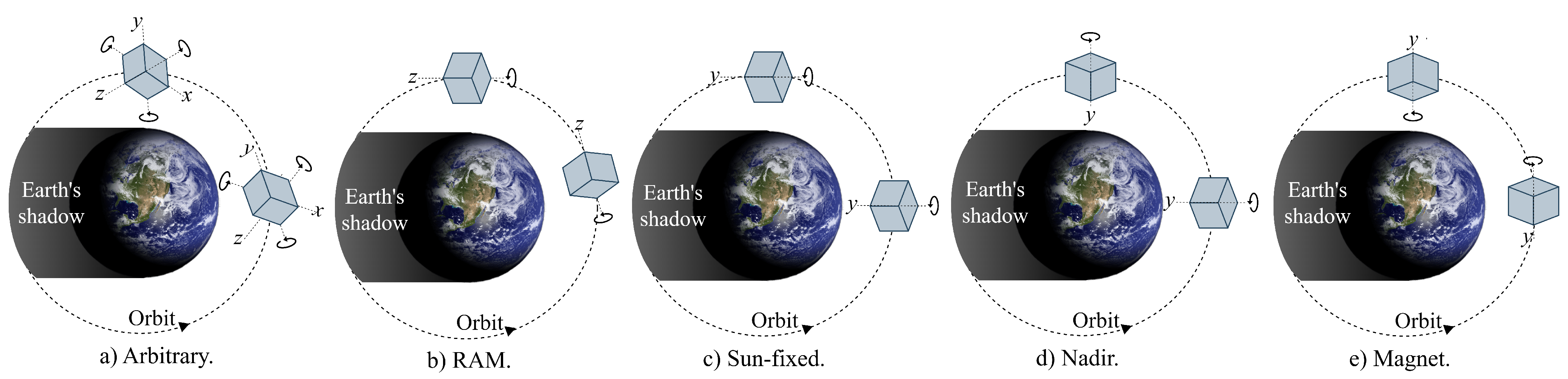
Attitude refers to the pointing direction of the spin axis in satellites [
17]. Even if the sun shines on the spacecraft, the absorption of solar radiation is a function of the attitude. Therefore, nanosatellites on identical orbits may have surfaces under different scenarios of solar flux as a consequence of their attitudes, e.g., some arbitrary spin, RAM (the spin axis is aligned with the velocity vector), sun-fixed (one or more sides constantly towards the sun), nadir (one or more sides constantly towards the center of the earth) or magnet (here referring to the state obtained by passive attitude control where the nanosatellite follows the earth’s magnetic field).
Figure 1 illustrates these attitudes.
For any attitude and any type of satellite, the projection of a surface k of the nanosatellite towards the sun, or in other words, its view factor, may be summarized by the parameter . Its value is between 0 (normal vector of surface k does not “see” the sun) and 1 (normal vector of surface k perfectly aligns with solar rays). Any other orientation will result in intermediate values (ignoring possible self-shadowing among the nanosatellite’s parts).
To simulate the attitude, the initial nanosatellite’s orientation and mass distribution must be known, and the forces and torques acting on it are integrated. To simplify this process, a pseudo attitude response may be obtained by specifying rotations for the satellite’s axis instead of solving the differential equations that govern it. This method is adopted here so a rotation matrix B and angles are informed by the user to obtain the spin of the nanosatellite.
To exemplify this process, the attitude of the nadir will be further described here. Assuming a cubic shape, as those from CubeSat 1U, the vector of initial orientation of each side
k may be assumed as:
These directions will change with time as the nanosatellite completes the orbit so that one side always faces the earth (see
Figure 1d). Therefore, the orientation
in each side
k, on the perifocal frame of reference, can be calculated by:
where, for this specific case, the matrix of rotation is:
The parameter is a residual spin to keep the satellite rotating but still always facing the earth. For different scenarios of attitude, the user has to combine other rotations of matrices.
Once the directions of the sides along the orbit are known, they must be translated from the perifocal frame of reference to the geocentric equatorial frame of reference [
16]. Therefore:
Finally, the projection of any side
k results from the dot product between
and the solar position, given by:
3. Instance Generation
Considering all aspects presented in the problem formulation section, we now present the exact procedures to generate a realistic instance of the ONTS problem, from power calculation to tasks scheduling data.
3.1. General Procedure for Power Calculation
The basic process to determine the power input for the instances is presented in Algorithm 1. The inputs for sun irradiance (
G), solar cell efficiency (
), and solar cell area (
A), as well as a timestep, must first be entered into the code. The algorithm specifies a few conversion variables in the sequence that will be used later in the code. Algorithm 1 then calls Algorithm 2 (“inputOrbit”), which is used to convert Orbital Inputs (OI) provided in units of angle and to derive preliminary orbital parameters that will later be used. A Newton–Raphson-based subfunction called “kepler_E” (Algorithm 3) is included in this algorithm to compute the eccentric anomaly (
E). It is important to note that the parameter
, which serves as a stopping point for convergence in Algorithm 3, is a small positive integer. Algorithm 4 (solar_position) is executed following Algorithm 2 to determine the sun’s position (
) for a particular day [
16]. When Algorithms 2 and 4 are complete, the loop in Algorithm 1 starts, and each iteration updates the time, the satellite’s position (
), the eclipse status (
), the attitude (
), the view factor (
F), and the power generation (
P) for each side of the CubeSat. When a full orbit’s period is reached, the loop comes to an end.
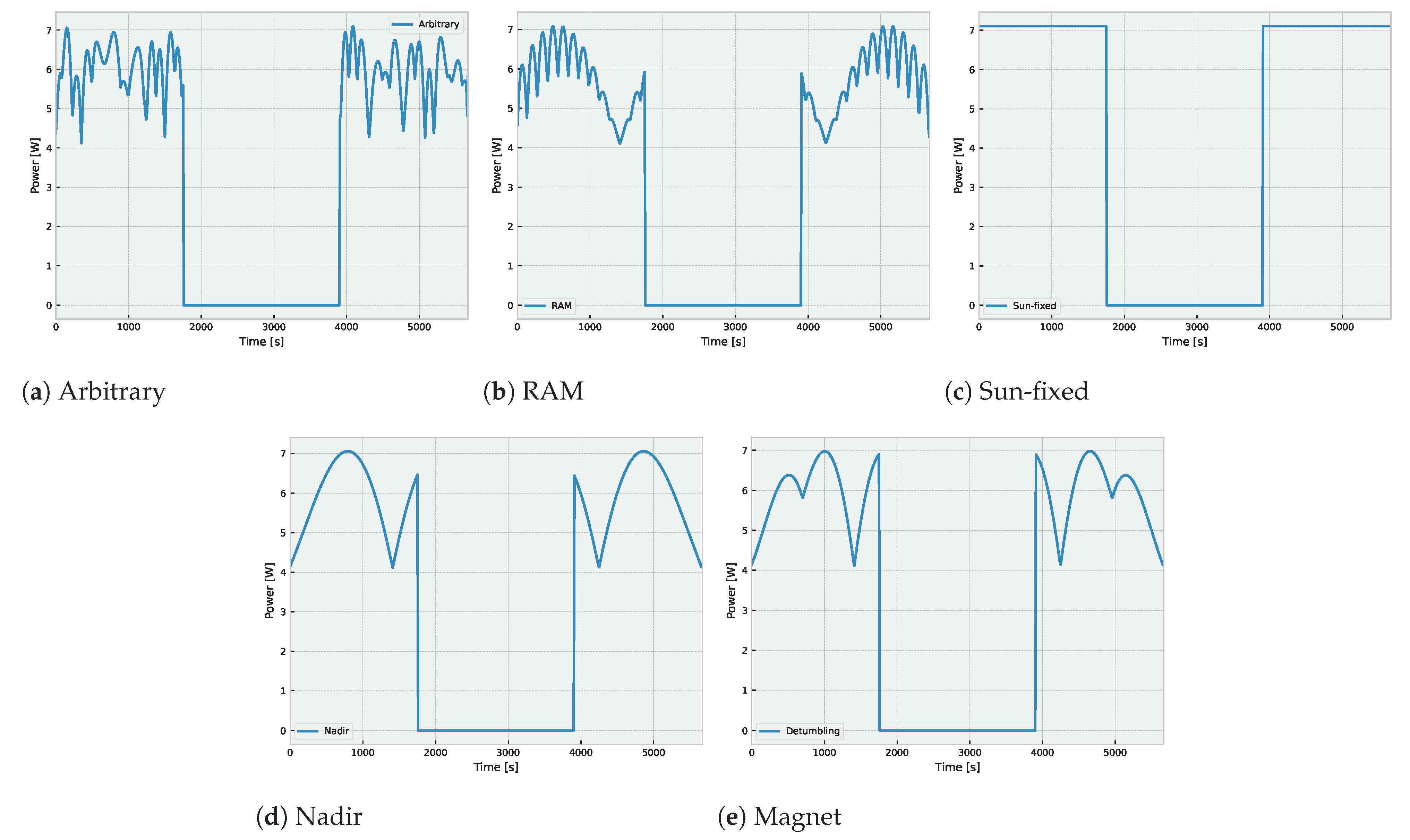
Five different results for power generation are illustrated in
Figure 2. Except for the attitude, they have the following common parameters:
,
,
,
,
, and
rev/day (equivalent to the altitude of 500 km), valid for 21 March 2023.
| Algorithm 1: General power calculation procedure |
![Data 08 00062 i001]() |
| Algorithm 2: Function—inputOrbit |
Input:
Output: - 1.
rad; - 2.
rad; - 3.
rad; - 4.
rad; - 5.
rad; - 6.
- 7.
- 8.
- 9.
- 10.
- 11.
|
| Algorithm 3: Function—kepler_E |
![Data 08 00062 i002]() |
| Algorithm 4: Function—solar_position | |
| Input: day, month, year | |
| Output: | |
| /* Compute Julian day | */ |
| 1 jd | |
| /* Astronomical unit (km) | */ |
| 2 AU ← 149597870.691 | |
| /* Julian days since J2000 | */ |
| 3 n ← jd - 2451545 | |
| /* Julian centuries since J2000 | */ |
| 4 cy ← n/36525 | |
| /* Mean anomaly (deg) | */ |
| 5 M ← 357.528 + 0.9856003 × n | |
| 6 M ← mod(M,360) | |
| /* Mean longitude (deg) | */ |
| 7 L ← 280.460 + 0.98564736 × n | |
| 8 L ← mod(L,360) | |
| /* Apparent ecliptic longitude (deg) | */ |
| 9 ← L + 1.915 × sin(M) + 0.020 × sin(2 × M) | |
| 10 ← mod(,360) | |
| /* Obliquity of the ecliptic (deg) | */ |
| 11 ← 23.439 - 0.0000004 × n | |
| /* Unit vector from earth to sun | */ |
| 12 | |
| /* Distance from earth to sun (km) | */ |
| 13 | |
| /* Geocentric position vector (km) | */ |
| 14 | |
3.2. General Procedure for Scheduling Data
The main objective here is to generate an ONTS instance based on random but realistic data for any mission size and orbit duration. The instances can be made more difficult to schedule on demand by increasing the number of jobs or time units to consider. For that we created the instance generator procedure presented in Algorithm 5. It takes two inputs: the number of jobs (
J) and the number of time units to be considered (
T). The output of the algorithm is the values for nine variables for each job:
,
,
,
,
,
,
,
,
, and
. This fully characterizes an instance for the ONTS regarding the QoS aspects.
| Algorithm 5: Instance generator algorithm |
![Data 08 00062 i003]() |
4. Data Validation
A few studies have already been conducted and published using the instance generation methodology presented here—although never previously explained in detail—demonstrating they are realistic and representative of the problem [
4,
5,
6,
7,
8]. In [
4], for instance, the authors propose a set of instances for the ONTS problem [
18]. These instances were designed to evaluate the performance of their branch-and-price (B&P) method for solving the ONTS problem. The cases are based on the FloripaSat-I mission, which is a nanosatellite with a 628 km altitude and a 97 minute orbit period. The amount of time units
T varies, where for values greater than 97 the extra units indicate alternative orbits or a finer time resolution—for example, scheduling in 30 second time steps. Furthermore, because the number of tasks directly correlates with the activation and deactivation timings of payloads on a nanosatellite, they reflect varying spacecraft sizes given that a larger volume may accommodate more payloads.
We now present the results of applying [
4] scheduling approach on data generated using the methodology presented here. First, the orbital characteristics of the FloripaSat-I mission, as presented in
Table 3, were used as input data for the power harvesting computation, and the power available for tasks was obtained by multiplying the power vector by an Electrical Power System (EPS) efficiency of
.
Then, a random instance was generated using Algorithm 5 with
and
as input. The output parameters are shown in
Table 4.
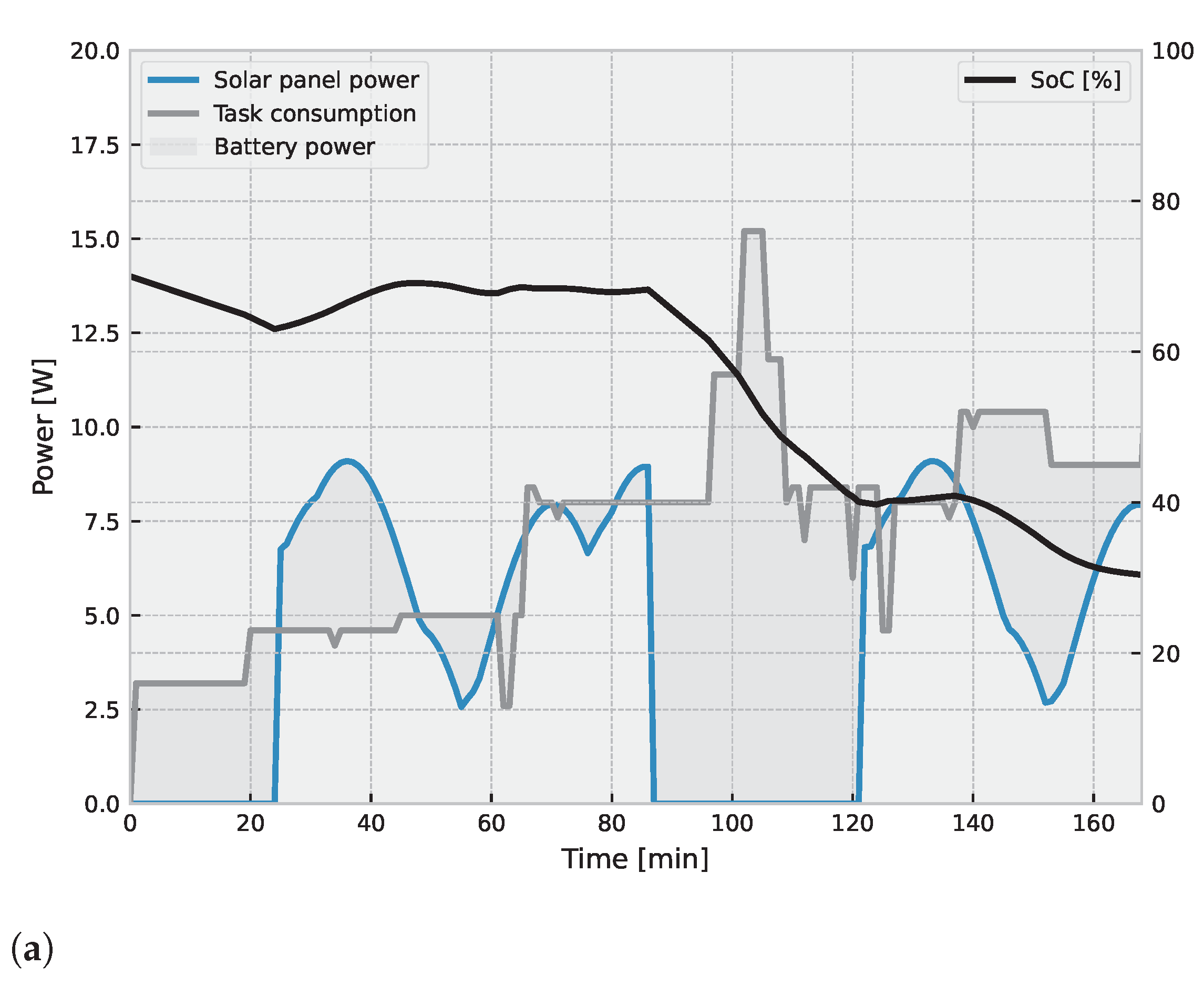
Finally, we attributed values to the battery and power management system parameters considering a 3U size nanosatellite, as presented in
Table 5.
Figure 3 shows the optimal schedule calculated for this example and the power analysis. The battery behavior along the orbit is shown in black, representing the State-of-Charge (SoC) at each moment. Notice that the battery power in gray can be power going to or coming from the battery, depending on the energy balance. The power input available to the tasks is shown in blue, including the eclipse time (0 W). One can notice how the battery SoC drops in eclipse time, where there is also an increase in tasks running, consuming more power.
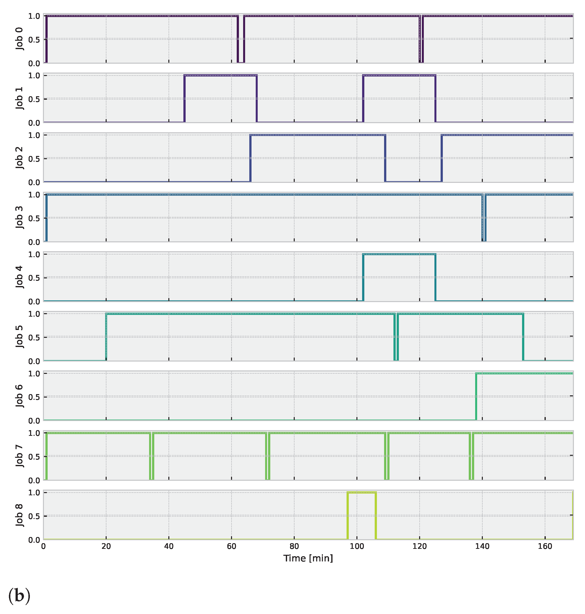
Figure 3b shows tasks from 0 to 8 where the x-axis goes from 0 to time
T, and the y-axis shows whether the task is on or off for each unit of time. When comparing this scheduling with parameters of
Table 4 it can be seen that they were followed accordingly. Job 5, for instance, cannot run before time 30 (
) and after time 153 (
), and so it was not.
5. Conclusions
In conclusion, this work offers a collection of cases of the Offline Nanosatellite Task Scheduling (ONTS) optimization problem. These instances were built using genuine input data based on the orbital characteristics of the FloripaSat-I mission and power harvesting calculations. They were created primarily to benchmark the performance of different solution approaches for the ONTS issue. The cases are intended to be scalable in size and complexity. The authors emphasize the need to share examples to ensure scientific research repeatability and provide a baseline for benchmarks in the ONTS problem.
Furthermore, this research emphasizes the crucial role of power budget prediction for successful nanosatellite mission planning and satellite job scheduling. Power budget estimation helps engineers make educated decisions about the number and type of payloads that may be put on the satellite, as well as offline scheduling algorithms to obtain the best times to activate and deactivate payloads, optimizing the use of available energy and mission extraction of value.
In other words, this study advances the area of nanosatellite scheduling by offering a collection of publicly available examples for researchers to utilize and compare their results against, as well as stressing the relevance of power budget prediction for optimal mission planning. As CubeSat missions are planned based on the data from our methodology, future work should be directed at validating and refining both the data and methods presented here.
Author Contributions
Writing—original draft preparation, C.A.R., E.M.F. and L.O.S.; writing—review and editing, L.L. and V.R.Q.L.; software, C.A.R., E.M.F. and L.O.S.; methodology, C.A.R., E.M.F. and L.O.S.; conceptualization, L.O.S.; supervision, L.O.S.; funding acquisition, L.L. and V.R.Q.L. All authors have read and agreed to the published version of the manuscript.
Funding
This work was supported by national funds through the Foundation for Science and Technology, I.P. (Portuguese Foundation for Science and Technology) by the project UIDB/05064/2020 (VALORIZA—Research Center for Endogenous Resource Valorization). The authors also acknowledge support from CNPq under grant numbers 404576/2021-4 and 150281/2022-6 and from FAPESC under grant number 2021TR001851.
Institutional Review Board Statement
Not applicable.
Informed Consent Statement
Not applicable.
Data Availability Statement
Conflicts of Interest
The authors declare no conflict of interest.
Abbreviations
The following abbreviations are used in this manuscript:
| ONTS | Offline Nanosatellite Task Scheduling |
| QoS | Quality of Service |
| EPS | Electrical Power System |
| B&P | Branch-and-Price |
| SoC | State-of-Charge |
Symbols
The following symbols are used in this manuscript:
| J | number of tasks. |
| T | number of time units. |
| priority of task j. |
| / | minimum and maximum running time required by task j. |
| / | minimum and maximum startups required by task j. |
| / | minimum and maximum period required by task j. |
| / | start and finish time of a task j execution window. |
| battery voltage, in Volts. |
| Q | battery capacity, in Ampere-hour. |
| battery level lower bound. |
| battery charge/discharge efficiency. |
| upper bound for battery discharge current, in Ampere. |
| energy harvested and available for tasks at time t. |
| power drained running task j. |
| i | orbit inclination in . |
| right ascension of the ascending node in . |
| e | eccentricity [-]. |
| argument of perigee in . |
| M | mean anomaly in . |
| mean motion in revolutions per day. |
| P | power generation. |
| power efficiency. |
| G | solar flux. |
| A | solar cell’s area. |
| F | view factor. |
| eclipse function. |
| position at the equatorial geocentric frame of reference. |
| position at the perifocal frame of reference. |
| Euler angle sequence. |
| h | specific relative angular momentum. |
| true anomaly. |
| gravitational parameter. |
| E | eccentric anomaly. |
| position of the sun. |
| initial orientation. |
| orientation at the perifocal frame of reference. |
| final orientation at the equatorial geocentric frame of reference. |
| matrix of rotation. |
References
- Villela, T.; Costa, C.A.; Brandão, A.M.; Bueno, F.T.; Leonardi, R. Towards the thousandth CubeSat: A statistical overview. Int. J. Aerosp. Eng. 2019, 2019, 5063145. [Google Scholar] [CrossRef]
- Shkolnik, E.L. On the verge of an astronomy CubeSat revolution. Nat. Astron. 2018, 2, 374–378. [Google Scholar] [CrossRef] [Green Version]
- Poghosyan, A.; Golkar, A. CubeSat evolution: Analyzing CubeSat capabilities for conducting science missions. Prog. Aerosp. Sci. 2017, 88, 59–83. [Google Scholar] [CrossRef]
- Rigo, C.A.; Seman, L.O.; Camponogara, E.; Morsch Filho, E.; Bezerra, E.A.; Munari, P. A branch-and-price algorithm for nanosatellite task scheduling to improve mission quality of service. Eur. J. Oper. Res. 2022, 303, 168–183. [Google Scholar] [CrossRef]
- Rigo, C.A.; Seman, L.O.; Camponogara, E.; Filho, E.M.; Bezerra, E.A. A nanosatellite task scheduling framework to improve mission value using fuzzy constraints. Expert Syst. Appl. 2021, 175, 114784. [Google Scholar] [CrossRef]
- Rigo, C.A.; Seman, L.O.; Camponogara, E.; Morsch Filho, E.; Bezerra, E.A. Task scheduling for optimal power management and quality of service assurance in CubeSats. Acta Astronaut. 2021, 179, 550–560. [Google Scholar] [CrossRef]
- Seman, L.O.; Ribeiro, B.F.; Rigo, C.A.; Filho, E.M.; Camponogara, E.; Leonardi, R.; Bezerra, E.A. An Energy-Aware Task Scheduling for Quality-of-Service Assurance in Constellations of Nanosatellites. Sensors 2022, 22, 3715. [Google Scholar] [CrossRef] [PubMed]
- Camponogara, E.; Seman, L.O.; Rigo, C.A.; Morsch Filho, E.; Ribeiro, B.F.; Bezerra, E.A. A continuous-time formulation for optimal task scheduling and quality of service assurance in nanosatellites. Comput. Oper. Res. 2022, 147, 105945. [Google Scholar] [CrossRef]
- Marcelino, G.M.; Morsch Filho, E.; Martinez, S.V.; Seman, L.O.; Bezerra, E.A. In-orbit preliminary results from the open-source educational nanosatellite FloripaSat-I. Acta Astronaut. 2021, 188, 64–80. [Google Scholar] [CrossRef]
- Marcelino, G.M.; Vega-Martinez, S.; Seman, L.O.; Kessler Slongo, L.; Bezerra, E.A. A Critical Embedded System Challenge: The FloripaSat-1 Mission. IEEE Lat. Am. Trans. 2020, 18, 249–256. [Google Scholar] [CrossRef]
- Ning, G.; Haran, B.; Popov, B.N. Capacity fade study of lithium-ion batteries cycled at high discharge rates. J. Power Sources 2003, 117, 160–169. [Google Scholar] [CrossRef]
- Li, J.; Gee, A.M.; Zhang, M.; Yuan, W. Analysis of battery lifetime extension in a SMES-battery hybrid energy storage system using a novel battery lifetime model. Energy 2015, 86, 175–185. [Google Scholar] [CrossRef] [Green Version]
- Gilmore, D.; Donabedian, M. Spacecraft Thermal Control Handbook: Fundamental Technologies; Spacecraft Thermal Control Handbook; Aerospace Press: El Segundo, CA, USA, 2002. [Google Scholar]
- Filho, E.M.; Seman, L.O.; Rigo, C.A.; Nicolau, V.P.; Ovejero, R.G.; Leithardt, V.R.Q. Irradiation Flux Modelling for Thermal–Electrical Simulation of CubeSats: Orbit, Attitude and Radiation Integration. Energies 2020, 13, 6691. [Google Scholar] [CrossRef]
- Vega Martinez, S.; Filho, E.M.; Seman, L.O.; Bezerra, E.A.; Nicolau, V.d.P.; Ovejero, R.G.; Leithardt, V.R.Q. An Integrated Thermal-Electrical Model for Simulations of Battery Behavior in CubeSats. Appl. Sci. 2021, 11, 1554. [Google Scholar] [CrossRef]
- Curtis, H.D. Orbital Mechanics for Engineering Students, 3rd ed.; Butterworth-Heinemann: Boston, MA, USA, 2014; p. 751. [Google Scholar] [CrossRef]
- Walter, U. Spacecraft Attitude Dynamics. In Astronautics: The Physics of Space Flight; Springer International Publishing: Cham, Switzerland, 2018; pp. 699–734. [Google Scholar] [CrossRef]
- Rigo, C.A.; Seman, L.O.; Filho, E.M. Nanosatellite Scheduling Instances. 2023. Available online: https://github.com/c-a-rigo/nanosatellite-scheduling-instances (accessed on 27 February 2023).
| Disclaimer/Publisher’s Note: The statements, opinions and data contained in all publications are solely those of the individual author(s) and contributor(s) and not of MDPI and/or the editor(s). MDPI and/or the editor(s) disclaim responsibility for any injury to people or property resulting from any ideas, methods, instructions or products referred to in the content. |
© 2023 by the authors. Licensee MDPI, Basel, Switzerland. This article is an open access article distributed under the terms and conditions of the Creative Commons Attribution (CC BY) license (https://creativecommons.org/licenses/by/4.0/).


 ,
, 


