Development of a Machine-Learning-Based Novel Framework for Travel Time Distribution Determination Using Probe Vehicle Data

Abstract

Investigating travel time variability is critical for pre-trip planning, reliable route selection, traffic management, and the development of control strategies to mitigate traffic congestion problems cost-effectively. Hence, a large number of studies are available in the literature which determine the most suitable distribution to fit the travel time data, but these studies recommend different distributions for the travel time data, and there is a disagreement on the best distribution option for fitting to the travel time data. The present study proposes a novel framework to determine the best distribution to represent the travel time data obtained from probe vehicles by using the modern machine learning technique. This study employs vast travel time data collected by fitting GPS tracking units on the probe vehicles and offers a comprehensive investigation of travel time distribution in different scenarios generated due to spatiotemporal variation of the travel time. The study also considers the effect of weather and uses the three most commonly used non-parametric goodness-of-fit tests (namely, Kolmogorov–Smirnov test, Anderson–Darling test, and chi-squared test) to fit and rank a comprehensive set of around 60 unimodal statistical distributions. The framework proposed in the study can determine the travel time distribution with 91% accuracy. Additionally, the distribution determined by the framework has an acceptance rate of 98.4%, which is better than the acceptance rates of the distributions recommended in existing studies. Because of its robustness and applicability in many different traffic situations, the proposed framework can also be used in developing countries with heterogeneous disordered traffic conditions to evaluate the road network’s performance in terms of travel time reliability.

1. Introduction

When urban commuters plan to use city road transportation, they are met with challenges from unanticipated factors, such as the level of congestion, the mix of traffic, accidents, incidents, weather changes, fluctuations in traffic demand, etc., which affect the anticipated travel time. Erratic changes on both the supply and demand sides of traffic introduce uncertainty in the travel time experienced by commuters. Because of this travel time uncertainty, the precise travel time of a trip is generally not known until it is completed, despite major improvements in urban transportation infrastructure and accessibility to many forms of transportation. As a result, commuters frequently plan their trip’s departure time, mode, and route based on only their prior experience from multiple travels.

Travel time variability makes trip planning even more challenging for travelers who do not have any prior experience of traveling in the area. Users see travel time variability as a risk (or added expense) to their travel decisions because it increases the uncertainty of arriving at their destination on time. It has been found experimentally that TTV is either the most important or the second most important factor for the majority of commuters [1]. Travel time variability significantly influences the users’ travel decisions, such as the choice of departure time [2,3], route choice [4,5], and mode choice [6,7]. Additionally, according to a study by Bates et al. [8], a reduction in travel time variability (TTV) is much more valuable to commuters/travelers than a reduction in travel time. Because of the rising relevance of TTV, this research topic is receiving the attention of researchers all over the world.

This paper presents a thorough empirical investigation of travel time variability on urban roads (both interrupted and non-interrupted corridors) by studying the travel time distribution. Earlier, it was difficult to collect travel-time-related information on a large scale, but now it can be easily acquired via various data sources using modern enhanced traffic sensing technologies. These technologies include station-based traffic condition monitoring (using devices such as microwave sensors, loop detectors, and video cameras) and point-to-point travel time measurement (e.g., probe vehicles, mobile, Bluetooth, license plate recognition systems, and automatic vehicle identification systems). The spatial arrangement and fixed positioning of traffic sensors significantly impact the data collection performance of station-based technologies. On the other hand, probe vehicles fitted with GPS tracking units might move over the entire road network and periodically collect the locational information of the vehicles and travel time data at regular intervals. The data obtained from the probe vehicles are referred to as probe vehicle data and represent relatively comprehensive operating characteristics for urban traffic. The data fidelity and coverage of anonymous probe vehicle data have improved significantly recently, making it a dependable data source for travel time studies. In the present study, probe vehicle data are used to investigate how travel time varies with the different weather conditions, type of road, the direction of the travel, day of the week (DOW), and time of the day (TOD).

A number of studies examining the travel time distribution are available in the literature and are listed in

Table 1. Travel time distribution studies available in the literature.

Study	Year	Location	Data Source	Dataset Duration/Size	Types of Vehicles Considered	Recommended Distribution	Limitations
[9]	1979	Chicago, USA	Drivers who measured TT on their regular daily trips to and from work	179 trips on 14 routes	-	Gamma	Considered only 179 trips
[10]	2009	Melbourne, Australia	GPS-equipped buses	3351 trips	Buses	Normal (peak hour) Lognormal (off-peak)	Considered travel time data of only buses and used a small dataset (only 3351 trips)
[11]	2009	Hirakata City, Japan	Buses operated by Keihan Bus Company	12 Days	Buses	Lognormal	Considered travel time data of only buses
[12]	2013	Adelaide, Australia	GPS-equipped probe vehicles	180, 67 runs for Route 1 and Route 2, respectively	N/A	Burr Type XII	Used a very small travel time dataset
[13]	2014	Beijing, China	Historical floating car data	Seven days	N/A	Generalized extreme value (GEV) and generalized Pareto	Used travel time data of one week only
[14]	2015	Brisbane, Australia	Transit Signal Priority (TSP) data	1 year	Buses	Lognormal	Considered travel time data of only buses
[15]	2016	Brisbane, Australia	TransLink Division, Department of Transport and Major Roads (DTMR)	6 months	Buses	Gaussian mixture	Considered travel time data of only buses
[16]	2018	Beijing, China	Taxis equipped with GPS devices (Probe Vehicles)	1 week	Taxis	Lognormal	Used travel time data of one week only, also used only taxis as probe vehicles
[17]	2018	Surat and Ahmedabad City, India	Video graphic survey	5 h a day for two working days	Two-wheelers, Three wheelers, cars, buses, LCVs, Truck	Burr	Used travel time data of 10 h only
[18]	2018	Surat, Mysore, and Chennai, India	SITILINK Ltd., Metropolitan Transport Corporation (MTC), Karnataka State Road Transport Corporation (KSRTC)	N/A	Buses	GEV	Considered travel time data of only buses
[19]	2018	Calgary, Alberta, Canada,	Calgary Transit	From 6 a.m. to 9 a.m. for six months	Buses	Lognormal (For pseudo horizon range = 7–8 km), Normal (For pseudo horizon range > 8 km)	Considered travel time data of only buses that also for morning peak only
[20]	2019	Nanjing, China	RFID Base Stations	One month	N/A	Gaussian mixture model	Used travel time data of one month only
[21]	2020	Surat, India	Video graphic survey	5 h	N/A	Burr (2 Lane), Log-logistic (3 Lane)	Used travel time data of 5 h only
[22]	2020	Charlotte, North Carolina, USA	Regional Integrated Transportation Information System (RITIS)	N/A	N/A	Burr	Used aggregated travel time data Dataset description, i.e., dataset duration and types of vehicles considered, is missing
[23]	2020	Mysore, India	KSRTC	4 months	Buses	Normal (peak hours), GEV (off-peak conditions)	Considered travel time data of only buses and used dataset of only four months
[24]	2020	New York City, USA	Department of Transportation, New York City, USA	8:00 a.m. to 8:00 p.m. for one week	N/A	Gamma Mixture	Considered travel time data for only one week
[25]	2021	Athens, Greece	Vodafone Innovus S.A	Three months	Passenger cars, taxis, minivans, vans, minibuses, buses, mini trucks	Lognormal	Considered travel time data for three months only
[26]	2021	Mysore, India	KSRTC (public transport)	Two months	Buses	GEV	Considered travel time data of only buses and used dataset of only two months
[27]	2022	Tehran, Iran	Wi-Fi and Bluetooth sensors	Two months	N/A	Lognormal	Considered travel time data for two months only

. Table 1 also summarizes the location, data source, dataset duration/size, vehicle types considered, recommended distribution, and limitations of these studies.

As we reviewed the available literature on travel time distribution, we found some significant weaknesses in previous research. The first limitation is that different distribution types, such as normal [10], lognormal [10,11,14,16,19,25], gamma [9,24], and Burr [17,21,22], etc., are fitted to travel time data, and there is disagreement on the best distribution option for fitting to travel time data.

The second limitation is that most of the studies considered only homogeneous traffic flow conditions, while disordered heterogeneous traffic flow conditions, which are common in developing nations [28] such as India, Sri Lanka, Bangladesh, Pakistan, Bhutan, Nepal, and others, are largely under-explored. Heterogeneity here refers to the variety of vehicle categories present in the traffic flow. The traffic flow in developing nations comprises a large variety of vehicles, ranging from non-motorized vehicles to light motorized vehicles (two-wheelers, three-wheelers, cars) to heavy vehicles (buses, trucks). Additionally, each of these vehicles has distinctive static and dynamic characteristics that, in turn, result in large variations in their driving behavior. For example, motorcycle riders will behave differently than bus drivers because motorcycles are smaller in size and have more maneuverability in comparison to buses. Additionally, disordered traffic is distinguished by a higher degree of lateral movements, excessive overtaking, occurrences of abrupt cuts in front of other vehicles, and staggered following (a vehicle following two leaders and positioned in between them). It is quite likely that this diversity in the vehicle categories and disorderly movement will lead to distinct travel time distributions and an increase in travel time variability.

Additionally, the limited studies [26,29] conducted in developing countries used the data from public transportation vehicles (buses) only. Additionally, as pointed out by a study by Kieu et al. [30], travel time data collected from public transportation vehicles are not a realistic representation of the actual travel time data, especially in terms of variability, due to the buses’ requirement to stick to schedules, bus queuing time, acceleration/deceleration time, dwell time, etc. Additionally, as stated previously, these vehicles’ drivers will behave differently in disordered heterogeneous traffic conditions. Moreover, the inclusion of travel time data from almost all vehicle types present in the traffic flow in the present study is expected to provide a comprehensive picture of travel time variability and assist policymakers in formulating policies for mitigating traffic congestion.

Additionally, we also observed that most of the research did not use a large dataset (say, data spanning a year). A large dataset can capture more variability and help in identifying a more realistic distribution that fits the travel time data.

Inspired by the limitations of previous studies, this study aims to build a machine-learning-based novel framework to determine the statistical distribution suitable to model travel time variability, especially in developing nations. The present study considers a comprehensive set of around 60 distributions to find the optimum/best fit for travel time data obtained from a large GPS trajectories dataset collected over a period of one year by installing GPS tracking devices on almost all vehicle types present in the disordered heterogeneous traffic streams seen in many developing nations. The present study is the most comprehensive study on travel time variability as it examines the effects of all factors affecting the travel time variability, including weather conditions, type of the roads, the direction of the travel, time of the day (TOD), and the day of the week (DOW).

This paragraph outlines how the rest of the manuscript is organized. Section 2 describes the data collection procedure and pre-processing steps taken to acquire the travel time data employed in the current study. Section 3 explains the approach used in the current study to build a machine-learning-based novel framework for travel time distribution determination. This section also provides an overview of the extent and pattern of travel time variation in heterogeneous disordered traffic streams, which is common in developing nations. Section 4 provides the details of the results obtained from fitting the statistical distributions using Easy Fit software and the development of the RUS Boosted decision-tree-based model for the travel time distribution determination. This section also includes a discussion related to the salient findings of the study. Lastly, Section 5 includes the conclusion drawn from the results obtained in the present study. Limitations and suggestions of the present study are also included in this section.

2. Study Area and Data Collection

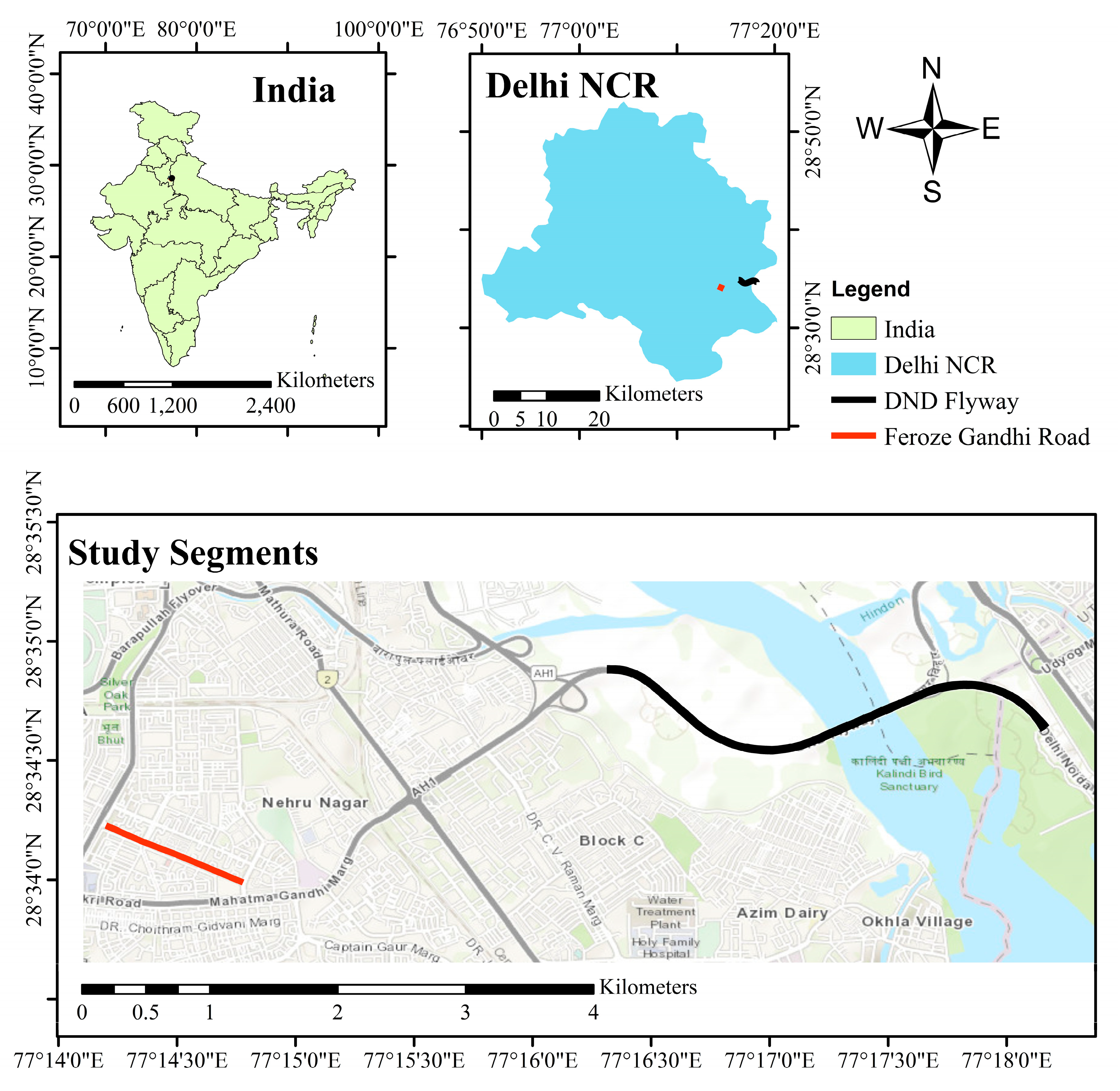
2.1. Study Area

In the present study, Delhi, also known as the National Capital Territory of Delhi (NCT), is selected as a study area. Delhi is a city and union territory that houses New Delhi, the nation’s capital. Its population is 16.7 million (according to the census of India, 2011), and the number of registered vehicles is over one crore (according to the Transport Department of NCT of Delhi, 2017). For the present study, two road segments representing uninterrupted and interrupted flow in the urban corridor, falling on Delhi-Noida Direct Flyway and Firoze Gandhi Road, respectively, are selected. The location map of the study area is shown in Figure 1.

DND Flyover is the primary connecting facility between Delhi and Noida, a major metropolis in the neighboring state of Uttar Pradesh. The freeway segment selected between the DND Toll, located in the Uttar Pradesh state of India, and Gol Chakkar Park, located in the Union Territory of Delhi, is an access-controlled uniform section and represents uninterrupted traffic flow in the urban corridor.

Feroze Gandhi Road is 1.19 km long and located in South East Delhi. This road experiences side friction due to its passage through the market area and represents interrupted traffic flow in the urban corridor in the true sense. Frequent traffic jams are also observed on this road which introduce significant variability in the travel time observed on this road.

2.2. Data Collection

Data for the current study were obtained from an Indian GPS tracking unit manufacturing firm. The firm shared the anonymized GPS trajectories of 2000+ vehicles permanently equipped with GPS tracking units and running in the study region for around one year. In GPS trajectories obtained, vehicle identification information was encrypted to protect the privacy of the vehicle owners. GPS trajectories utilized in the study consisted of different types of vehicles such as personal cars, taxis, commercial vehicles, etc., covering almost all vehicle types present in the traffic of developing nations.

Raw data obtained in the form of GPS trajectories consisted of the following information: encrypted device ID, timestamp, locational information (latitude, longitude, altitude), directional information (bearing), engine status (ON/OFF), and speedometer information (vehicle instantaneous speed). A sample of the raw dataset is shown in

Table 2. A sample of the raw data obtained from GPS tracking devices.

Encrypted Device ID	Timestamp	Latitude	Longitude	Altitude	Bearing	Engine Status	Speedometer Reading
8493	31-07-2018 03:20:54	28.65647095	77.43452638	204	0	1	0
458	31-07-2018 03:20:53	28.66622667	77.32199333	N/A	16.34	1	60.5
459	31-07-2018 03:20:51	28.646855	77.41362333	N/A	36.6	1	36.6
8487	31-07-2018 03:20:50	28.64896978	77.34511459	187	0	1	0
12533	31-07-2018 03:20:52	28.68999299	77.35131744	196	241	0	0

.

Raw weather data for the current study were obtained from the website www.wunderground.com (accessed on 2 September 2022). This website provides historical meteorological data, such as temperature, pressure, wind speed, precipitation, visibility, etc., for the required time frame.

According to past studies, it is widely acknowledged that only bad weather substantially impacts travel times and speeds. Hence, detailed weather conditions are further classified into only two categories, i.e., interfering and non-interfering weather conditions.

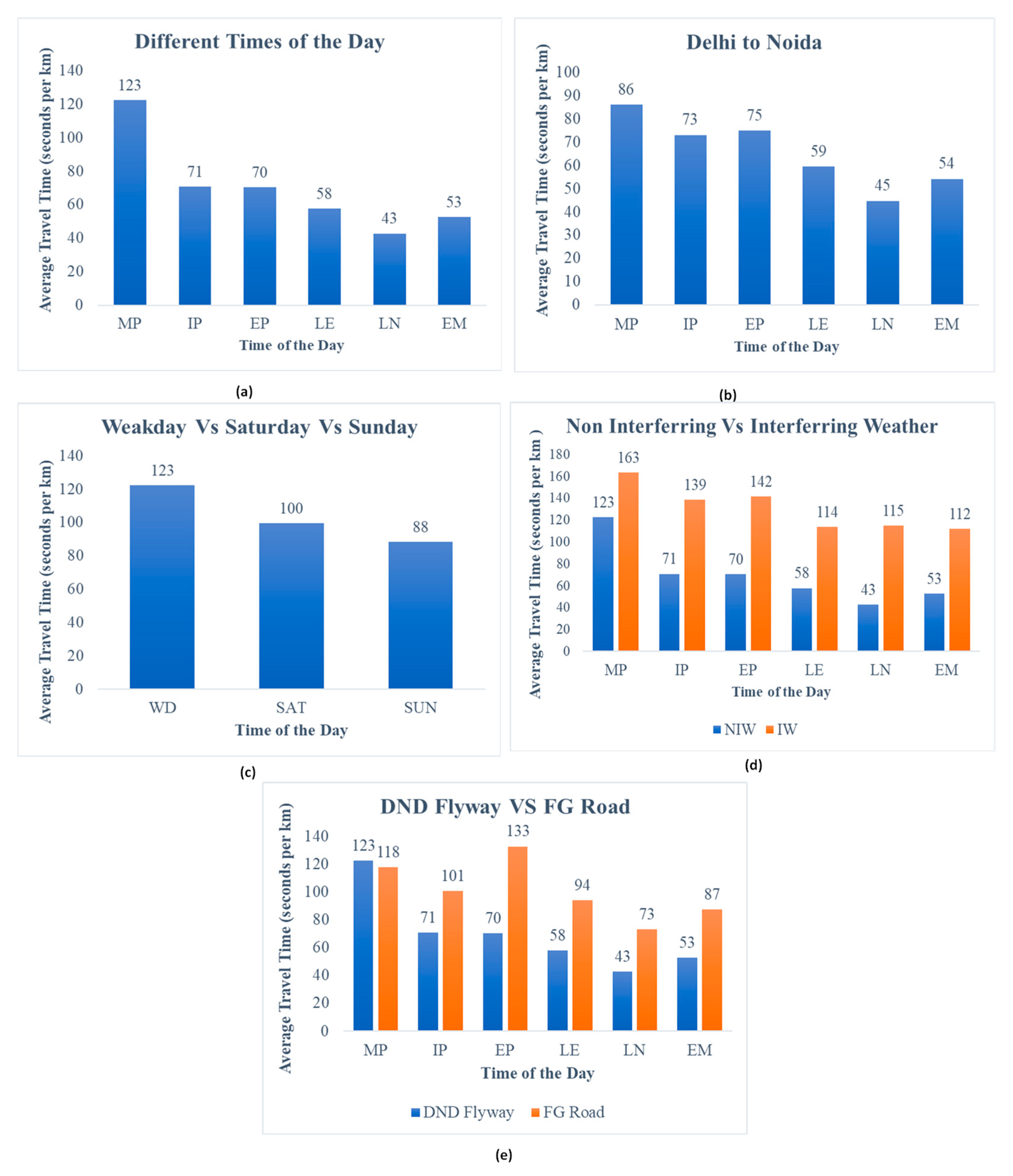
• Non-Interfering Weather Conditions: Weather conditions such as fair, partly cloudy, mostly cloudy, cloudy, haze, smoke, and blowing dust have no discernible effect on the traffic conditions. Hence, these are grouped into the non-interfering weather conditions class.
• Interfering Weather Conditions: all weather situations, such as drizzle, light rain, rain, heavy rain, thunderstorm, mist, shallow fog, fog, etc., that are expected to have a considerable effect on travel times and speed. Hence, these are grouped into interfering weather conditions class.

2.3. Data Pre-Processing

Data pre-processing includes various steps required to transform the raw GPS trajectories into useful travel time data. These steps include data cleaning, trip extraction, and map matching and are described in detail in this sub-section.

2.3.1. Data Cleaning

Encrypted raw data obtained from the firm were cleaned using usual data cleaning approaches, such as the removal of duplicate points with identical IDs and timestamps.

Although the probe vehicles’ GPS tracking units can measure the locational information with high accuracy, the data obtained from these devices contain a significant number of outliers for a wide range of reasons, such as multipath signals, signal loss, atmospheric interference, etc. Therefore, these outliers were removed before proceeding further. In the current study, GPS points with an instantaneous speed of more than 120 km/h are regarded as outliers and removed from the dataset; 120 km/h is the maximum speed for which roads are designed in the study area.

2.3.2. Data Visualization and Trip Extraction

In the literature, there are several methods for identifying the trips from the trajectories, e.g., temporal gaps (e.g., no change in the location for a minimum of 15 min), recurring patterns (e.g., daily journeys), positional features (e.g., whether the engine is on/off), extensive movement (e.g., if the next location is more than 5 km away), etc. The current study used tableau software for visualizing the data and extracting the trips falling on the study segments. Finally, travel time data with the direction of travel were obtained by comparing the arrival and departure times of the vehicles in the study segment. A total of 52,569 trips were obtained on both study segments by following the above-mentioned approach.

The trips having travel time longer than walking time are regarded as outliers. In the current study database, 38 trips matched this outlier criterion. Hence, these were removed to obtain the final travel time data utilized in the current study for the distribution fitting.

3. Methodology

The different steps involved in the development of a novel framework for travel time distribution determination are shown in Figure 2.

3.1. Analysis and Classification of Data

The first step in determining the best-fitted distribution is to classify the data into various classes representing different traffic conditions. This classification can be carried out based on the variability range of the degree of capacity utilization. However, as the present study proposes to develop the framework based on only the GPS trajectories of the probe vehicles, the variation of the travel time per unit length, which is an indirect measure of the degree of capacity utilization, is used for the classification of the data. Hence, in the first step toward the development of the framework for travel time distribution determination, the travel time variation with the type of road, the direction of the travel, the day of the week (DOW), the time of the day (TOD), and weather conditions were analyzed. Figure 3 shows the sample of the travel time variation obtained from the data used in the current study.

Figure 3a,b show the trend of the travel time variation with the time of the day on weekdays (working days) for DND Flyway during non-interfering (normal) weather conditions in the directions Noida to Delhi and Delhi to Noida, respectively. From these figures, it can be inferred that travel time varies with the time of the day, and time of the day can be classified into five classes, viz., Morning Peak (MP) from 9:00 to 11:00, Inter Peak (IP) from 11:00 to 16:00, Evening Peak (EP) from 16:00 to 20:00, Late Evening (LE) from 20:00 to 1:00, Late Night (LN) from 1:00 to 6:00, and Early Morning (EM) from 6:00 to 9:00. Additionally, the travel time of the trips varies with the direction of the travel. Hence, both directions shall be considered separately to study and model the travel time variability.

Figure 3c shows the travel time variation with the day of the week for DND Flyway in the direction of Noida to Delhi during Morning Peak time in normal weather conditions. From this figure, it can be inferred that trips on working days have more travel time compared to off days (Sundays). Trips made on Saturdays have in-between travel time. The possible reason behind this observation could be that many businesses and offices in Delhi are off on Sundays only, while others have two off days (Saturdays as well as Sundays). Based on the travel time variation shown in Figure 3c, days of the week can be classified into three categories: working days (WD), Saturdays (SAT), and Sundays (SUN).

Figure 3d shows the comparison of the travel time variation during normal weather conditions and interfering weather conditions for DND Flyway in the direction of Noida to Delhi on weekdays. From this figure, it can be inferred that the travel time of the trips increases significantly during the interfering weather conditions. Hence, travel time variability shall be studied separately during normal and interfering weather conditions.

Figure 3e shows the comparison of the travel time in seconds per km on an uninterrupted urban corridor (DND Flyway) and an interrupted urban corridor (FG Road). From the figure, it can be inferred that during rush hours (morning peak), both roads behave at almost the same travel speed, but during non-rush hours, travel speed on the interrupted corridor is comparatively slow. Hence, travel time variability shall be modeled differently on interrupted and non-interrupted urban corridors.

Hence, based on the above inferences, travel time data were categorized into 144 categories (based on the type of road, the direction of travel, the day of the week, the time of the day, and weather conditions). As of the date this paper was written, we could not find any research that has taken such a comprehensive and detailed classification of travel time into account.

Table 3. Descriptive statistics for travel time data on uninterrupted urban corridor (DND Flyway).

Travel Direction	DOW	TOD	Non-Interfering Weather Conditions					Interfering Weather Conditions
			N	TMin	TMax	ATT	SD	N	TMin	TMax	ATT	SD
Noida to Delhi	Weekdays	MP	1625	165	547	441	60	386	170	810	588	137
		IP	3722	178	654	255	36	503	140	732	500	100
		EP	1751	159	640	253	42	264	193	705	510	100
		LE	2788	112	1192	208	63	650	121	591	410	81
		LN	1038	107	958	154	55	332	139	585	414	80
		EM	1311	146	556	189	37	251	101	536	403	78
	Saturdays	MP	749	168	489	359	52	58	257	673	499	94
		IP	749	188	529	271	42	101	103	707	480	94
		EP	322	173	521	256	41	49	226	695	494	107
		LE	369	129	499	218	57	87	187	573	411	79
		LN	221	116	681	165	67	55	165	565	433	76
		EM	330	160	493	191	28	63	225	569	415	68
	Sundays	MP	209	145	555	318	65	49	256	669	495	91
		IP	801	175	413	251	38	110	219	649	475	100
		EP	354	175	386	258	35	54	154	699	467	113
		LE	346	121	536	208	58	81	224	581	417	78
		LN	145	120	359	161	37	37	170	559	415	85
		EM	305	160	320	188	21	59	133	557	413	85
Delhi to Noida	Weekdays	MP	981	166	972	310	72	230	137	680	516	116
		IP	2513	181	740	263	44	343	102	669	491	96
		EP	2019	187	629	270	35	302	200	720	551	112
		LE	2164	124	933	214	57	508	157	582	425	77
		LN	966	115	577	161	50	242	165	596	431	81
		EM	1663	153	769	195	42	317	120	588	421	75
	Saturdays	MP	168	168	452	318	55	41	104	677	491	117
		IP	463	192	504	263	39	65	291	672	495	81
		EP	442	171	559	261	46	65	197	670	493	111
		LE	417	125	768	211	59	96	178	584	422	90
		LN	202	112	490	163	51	51	121	579	428	83
		EM	333	153	500	187	30	62	170	583	413	79
	Sundays	MP	159	126	481	301	59	36	214	674	497	95
		IP	466	163	427	246	40	64	195	639	474	98
		EP	480	166	527	253	43	71	195	662	492	103
		LE	410	106	748	205	54	97	212	568	440	73
		LN	192	117	493	169	57	49	155	591	438	68
		EM	324	166	293	191	18	65	148	575	406	87

and

Table 4. Descriptive statistics for travel time data on interrupted urban corridor (FG Road).

Travel Direction	DOW	TOD	Non-Interfering Weather Conditions					Interfering Weather Conditions
			N	TMin	TMax	ATT	SD	N	TMin	TMax	ATT	SD
UP	Weekdays	MP	617	63	200	140	22	145	134	255	213	22
		IP	1310	40	220	120	23	179	104	236	183	22
		EP	885	82	204	158	18	132	157	270	227	23
		LE	1004	98	195	112	9	235	135	261	219	23
		LN	323	70	218	87	18	81	93	215	165	24
		EM	649	91	162	104	7	124	137	243	198	22
	Saturdays	MP	122	39	192	124	29	29	123	219	184	21
		IP	290	59	177	116	19	38	135	210	177	18
		EP	176	77	194	162	18	26	171	256	224	22
		LE	190	94	151	108	9	46	150	250	212	28
		LN	51	68	148	83	12	14	120	198	168	22
		EM	125	92	161	103	9	24	154	236	204	23
	Sundays	MP	117	57	211	128	28	27	115	206	182	20
		IP	277	68	201	119	19	36	57	217	175	29
		EP	167	80	193	162	18	25	158	252	219	25
		LE	181	94	167	107	10	36	149	256	220	23
		LN	48	67	195	82	18	10	112	192	165	26
		EM	119	90	131	100	6	23	147	241	203	25
DOWN	Weekdays	MP	558	56	205	143	22	129	126	258	214	23
		IP	1184	46	208	122	24	160	97	227	182	24
		EP	796	88	205	160	18	122	165	264	225	21
		LE	906	97	233	112	10	212	128	271	218	21
		LN	291	64	188	80	14	73	82	213	158	25
		EM	586	95	173	107	7	112	118	249	196	25
	Saturdays	MP	121	70	191	127	25	28	105	208	182	22
		IP	284	83	180	126	17	39	115	216	180	21
		EP	172	104	202	164	19	26	184	261	223	20
		LE	185	94	186	109	10	44	157	259	220	20
		LN	49	65	202	81	20	13	87	190	151	30
		EM	122	96	150	105	9	24	137	241	197	22
	Sundays	MP	110	75	200	127	28	27	135	211	183	20
		IP	262	65	183	118	19	37	89	238	173	29
		EP	160	105	199	163	19	23	159	258	222	24
		LE	172	93	148	106	8	40	160	264	223	19
		LN	46	62	227	80	25	12	114	188	162	22
		EM	114	94	133	104	7	21	145	237	203	21

show the descriptive statistics of the travel time data obtained on interrupted and uninterrupted urban corridors, respectively.

Table 3 and Table 4 shows that travel time varies substantially even under free-flow conditions prevailing in the late night period of the day. This large variation hints towards the problem of heterogeneity in the traffic streams of developing nations. Additionally, a large variation in travel time is observed during traffic jam conditions. This is possibly due to the combined effect of heterogeneity and disorderliness prevalent in the traffic stream. From these observations, it can be inferred that traffic conditions in developing nations are different from those in developed nations, which have nearly homogeneous traffic with proper lane discipline.

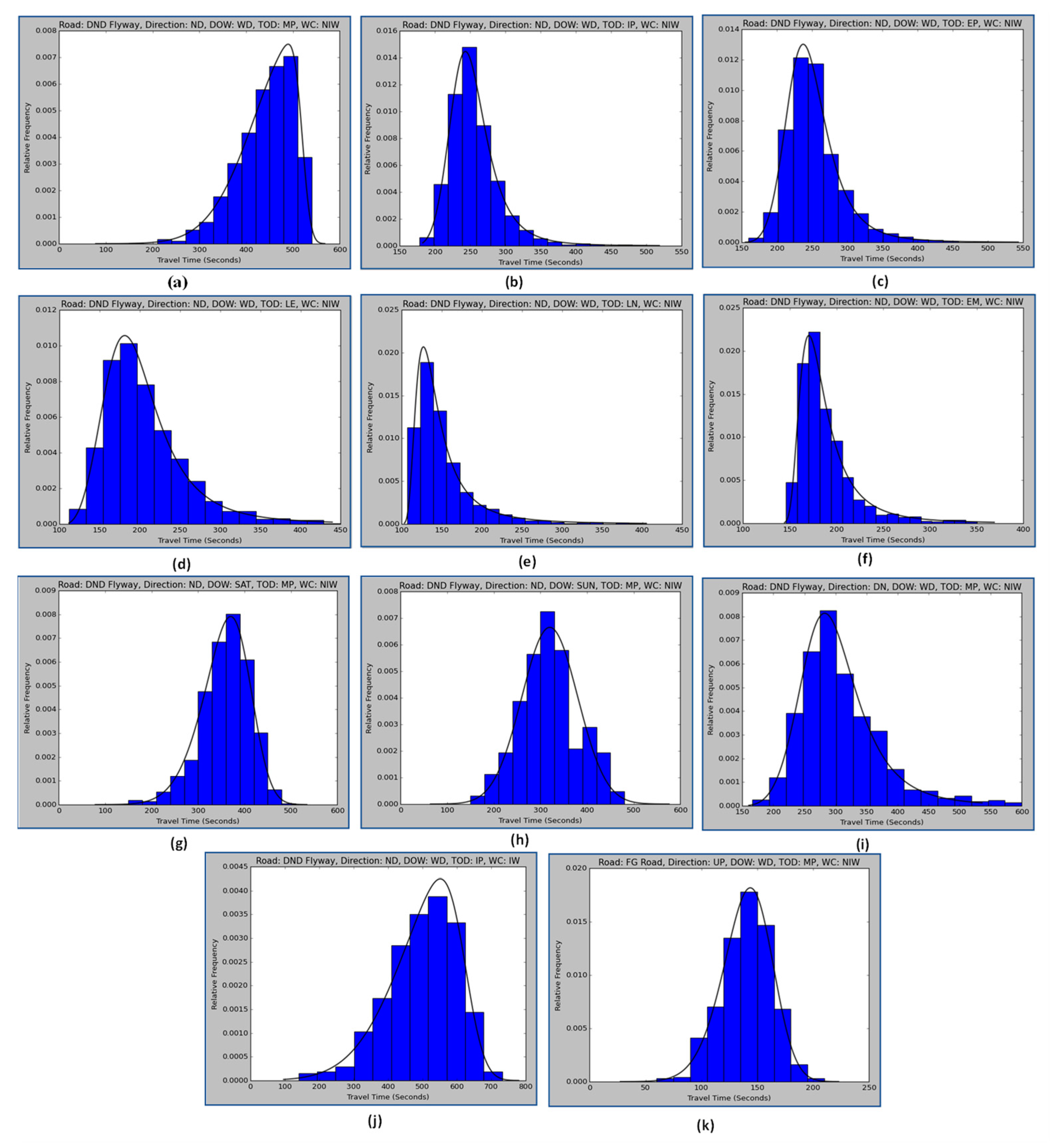
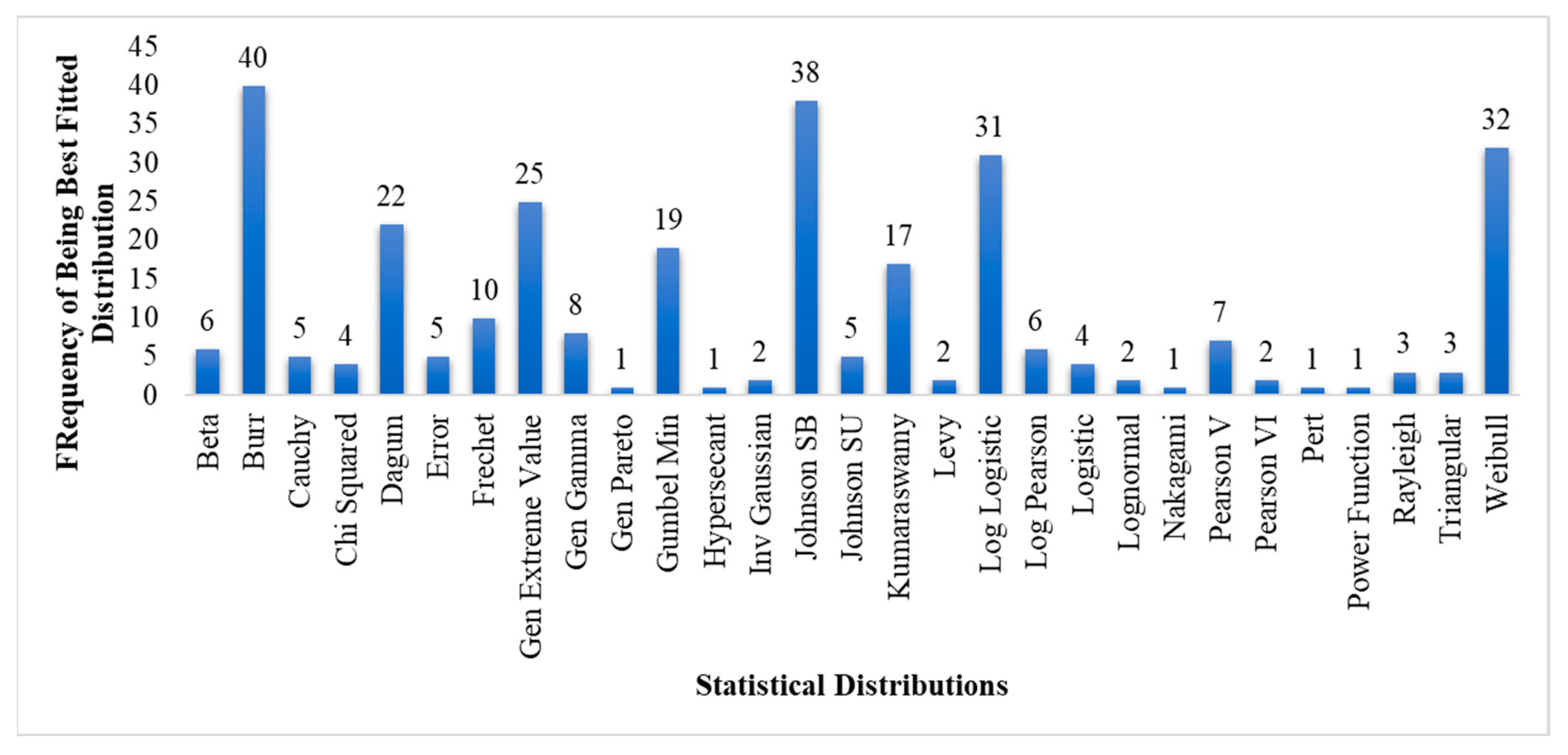
3.2. Distribution Fitting

Statistical distributions are fitted to each category’s observed travel time data in this step. In the present study, a comprehensive set of around 60 statistical distributions, including the most widely used distributions in the literature, such as Burr distribution, Gamma distribution, and lognormal distribution, is used to find which distribution can match the travel time data desirably. The current study also estimates the parameters of each distribution in each category. For the distribution fitting and their parameter estimation, the EasyFit software by math wave is used. EasyFit covers a wide range of continuous distributions, which are classified into the following four types (distribution types):

• Bounded Distributions: Distributions that fall into this category include Uniform distributions, Triangular, Reciprocal, Power Functions, PERT, Beta, and Johnson-Simons-Brown (JSB). These distributions are bounded between a range of [a,b].
• Unbounded Distributions: Normal, Logistic, Cauchy, Error, Error Function, Johnson SU, Hyperbolic Secant, Student’s t distribution, and Laplace (Double Exponential) are among the unbounded distributions. These distributions are unbounded and have a range of (−∞, +∞).
• Non-Negative Distributions: The majority of these distributions are defined for the range x > γ, which is equivalent to x − γ ≥ 0, where γ is a continuous location parameter. Log-logistic, Inverse Gaussian, Weibull, Levy’s Log-Gamma, Rayleigh’s Rice, Nakagami’s Lognormal, Pearson V, Pearson VI, Pareto (first kind), and Pareto (second kind) are among the non-negative distributions supported by the EasyFit software. Most of the non-negative distributions supported by EasyFit are available in two versions or forms: a simplified version and a complete version.
• Advanced Distributions: EasyFit’s classification of continuous distributions is based on various definitions. As a result, some of the continuous distributions do not fall into any of the categories listed above. Simultaneously, they frequently represent more valid models than a large number of other distributions. EasyFit supports advanced distributions such as generalized Pareto, generalized extreme value (GEV), Log-Pearson III, Wakeby, generalized logistic, Phased Bi-Exponential, and Phased Bi-Weibull. These distributions are generated by combining two or more basic distributions. For instance, the GEV distribution is generated by combining Weibull, Gumbel, and Frechet distributions.

For checking the goodness-of-fit, the three most widely used non-parametric tests, namely the Kolmogorov–Smirnov, Anderson–Darling, and chi-squared tests, are used.

3.2.1. Kolmogorov–Smirnov Test

Suppose the travel time dataset from particular traffic conditions consists of T₁, T₂… T_n as data points from some distribution with cumulative distribution function (CDF) F(x). Then, empirical CDF is defined as follows:

$$F_n\left(T\right)=\frac{1}{n}\times \left[Number of Observations \le T\right]$$

(1)

The following equation defines the Kolmogorov–Smirnov test statistic (D):

$$D=\underset{0\le i\le n}{\max } \left(F\left(T_i\right)-\frac{i-1}{n}, \frac{i}{n}-F\left(T_i\right)\right)$$

(2)

3.2.2. Anderson–Darling Test

In this test, tails are given more weight as compared to the Kolmogorov–Smirnov test. The following equation defines the Anderson–Darling (A-D) test statistics (A²):

$$A^2=-n-\frac{1}{n}\times {\displaystyle \sum }_{i=1}^n\left(2i-1\right).\left[lnF\left(T_i\right)+ln\left(1-F\left(T_{n-i+1}\right)\right)\right]$$

(3)

A-D test critical values typically depend on the particular distribution being evaluated. However, it is difficult to find tables of critical values for several distributions. EasyFit uses an approximation formula, which gives the same critical values for all distributions based on the sample size only. A-D test based on these same critical values for all distributions is less likely to reject a good fit than the original A-D test and can be used to compare several fitted distributions.

3.2.3. Chi-Squared Test

This test is used for continuous data only, and the test statistic’s value depends upon the data’s binning. Various formulas can be used to determine bin size based on the sample size (N). EasyFit software uses the following empirical formula to calculate the number of bins (k) and can group the data into intervals of equal width or probability.

$$k=1+{\log }_{2}N$$

(4)

The chi-squared test statistic (χ²) is defined as follows:

$${\chi }^2={\displaystyle \sum }_{I=1}^N\frac{{\left(O_i-E_i\right)}^2}{E_I}$$

(5)

Although, as per the original test, DOF (degree of freedom) is calculated as k-c-1, EasyFit calculates DOF as k − 1 since this definition reduces the chances of rejecting the fit in error. Hence, the critical value for the chi-squared test in EasyFit is defined as ${\chi }_{1-\alpha ,k-1}^2$.

Next, the fitted distributions are ranked based on the test statistics, and the best-fitted distributions are identified based on the test statistics values of the three tests as mentioned above for each of the 144 categories considered in the study.

3.3. Determination of Distribution Suitable for Travel Time Data

In order to determine the most appropriate statistical distribution for travel time under different traffic conditions, first, the data consisting of the best-fitted distribution with the corresponding test, type of the road, the direction of the travel, DOW, TOD, and weather conditions were split into the training (70%) and test (30%) dataset. Then, the five most popular distributions among the best-fitted distributions determined in the previous step were identified. Finally, the RUS Boosted ensemble classifier was trained on the training dataset using MATLAB to determine the travel time distribution for the instances in the test dataset. In the earlier studies, the distribution which has the highest acceptance rate is assumed to fit the travel time data in all scenarios. As the distribution with the highest acceptance rate need not be the best-fitted distribution, the authors think that the assumption of the highest acceptance rate distribution fitting to all scenarios made in earlier studies is unreasonable, especially in heterogeneous disordered traffic conditions.

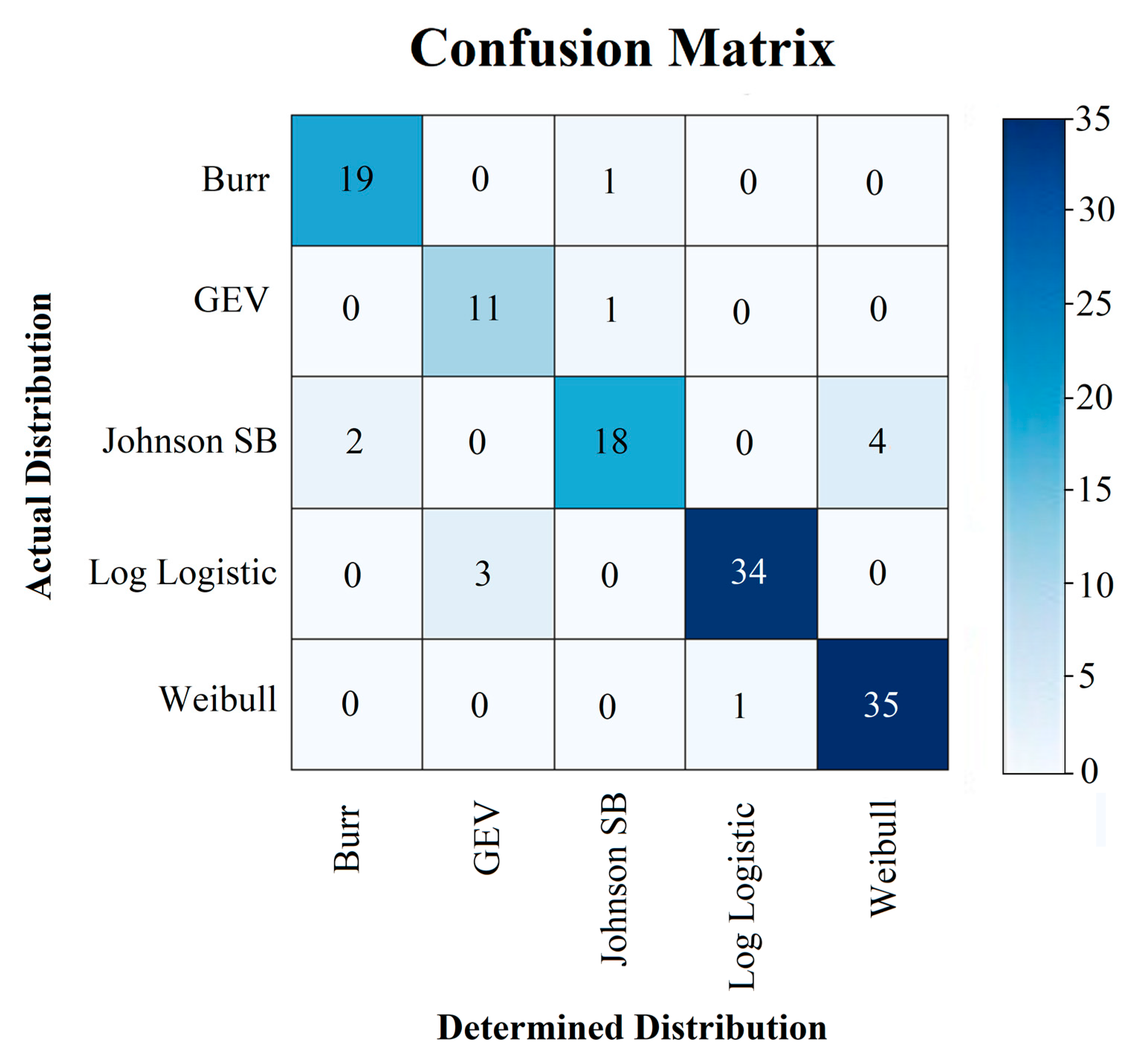
4. Results and Discussion

The authors observed that during the different traffic conditions, not only the average travel time but also the shape of the travel time distribution are different. Figure 4 shows the travel time histogram for different traffic conditions.

From Figure 4a it can be observed that the travel time distribution curve is left-skewed during rush hours. The left-skewed shape possibly represents that the drivers are forced to move slowly. On the contrary, the travel time distribution curve under the free flow condition shown in Figure 4e is right-skewed, which possibly indicates that drivers are free to drive at any speed they desire, and most of the drivers prefer to drive fast. The same statistical distribution cannot model these different shapes of the travel time distribution curve. From this observation, the authors infer that the studies available in the literature may also have considered different traffic situations, resulting in different distributions. Hence, there is disagreement on the best distribution option for fitting travel time data in the literature.

This study used a comprehensive set of around 60 statistical distributions to find the best-fitted distribution based on the test statics value of three commonly used tests (KS, AD, CS). Figure 5 shows the plot of the various statistical distributions fitted to the travel time data and the frequencies of their being the best-fitted distributions over the training dataset.

Figure 5 shows that the Burr, Johnson SB, Log Logistic, Weibull, and general extreme value (GEV) are the five most popular distributions among the best-fitted distributions over the training dataset. Analysis of the best-fitted distributions over the test dataset showed that these distributions are also the five most popular distributions over the test dataset. These distributions are also among the best-fitted distributions reported for the travel time data in the literature.

In the next step, the best-fitted distribution among the five most popular distributions (Burr, GEV, Johnson SB, Log Logistic, and Weibull) was determined for each of the 144 traffic situations generated based on the test statics values of tests mentioned earlier.

Finally, the RUS Boosted ensemble classifier was trained on the training dataset having the best-fitted distribution data with the corresponding road type, the direction of the travel, DOW, TOD, and weather conditions.

It was observed that data points of different distributions differ significantly, as expected. Hence, travel time distribution determination using a classifier has an issue of class imbalance. Therefore, the classifier employed for the travel time distribution determination needs to use data sampling/boosting techniques to alleviate the issue of class imbalance. Data sampling strategies modify the training dataset’s class distribution in an effort to address the issue of class imbalance. Random Under Sampling (RUS) used in the present study removes instances from the dominant class randomly until the required class distribution is reached.

In the present study, the RUS Boosted ensemble classifier is used. Ensemble classifiers aggregate the classifying capability of the individual classifiers. Decision tree ensembles are the most effective classifiers and can solve the instability issue of the decision tree. In ensemble classifiers, weak learners are run repeatedly on the training data and combined to give superior performance. These models generally have the problem of overfitting. So, five-fold cross-validation is used to protect the model against overfitting. Additionally, cross-validation is also utilized for tuning the model’s hyperparameter.

The model developed in the present study has a validation and test accuracy of 92.4% and 90.7%, respectively. The model has a training time of 3.8 s.

Table 5. Comparison of the present study with recent similar studies.

S. No.	Study	No. of Distributions Considered	Number of Traffic Scenarios Considered	Acceptance Rate
1	Present study	60	144	98.4%
2	[25]	7	6	91.6%
3	[16]	4	16	87.5%
4	[22]	4	24	79.2%

shows the comparison of the present study with similar recent studies available in the literature in terms of performance and robustness.

The present study determined the best-fitted travel time distribution with 90.7% accuracy, i.e., in 90.7% of the instances, the distribution determined by the model developed in the present study is the same as the best-fitted distribution. In the rest of the cases, it is the second or third best-fitted distribution. Here, it should be noted that the model proposed in the study gave the rejected distribution in only two instances.

Therefore, the acceptance rate for the distribution determined by the model developed in the present study is 98.4%. The model developed in the present study has an acceptance rate of 98.4%. Among the studies available in the literature, the study by Adnan et al. [25] determined the distribution with the highest acceptance rate (91.6%). So, in terms of acceptance of the TTD distribution recommended by the studies, the present study is better than the highest-performing study available in the literature.

Additionally, the present study is most robust in terms of the number of traffic scenarios and statistical distribution considered. Hence, the framework proposed in the current study can be utilized for widely varying traffic situations.

To further analyze the class-wise performance of the model, a confusion matrix was produced. Figure 6 shows the confusion matrix for travel time distribution (TTD) determined by the proposed framework over the test dataset.

In the classification tasks, classification can fall under any of the four categories, namely true positive (TP), true negative (TN), false positive (FP), and false negative (FN), as per the conditions defined below:

• Classification x_i is a true positive for class c if both the actual and the predicted classes of x_i are the same as c.
• Classification x_i is a true negative for class c if neither of the actual or predicted classes of x_i matches with c.
• Classification x_i is a false positive for class c if the predicted class of x_i matches c but the actual class does not.
• Classification x_i is a false negative for class c if the actual class of x_i matches c but the predicted class does not.

As the data points in all classes are not equal, to further evaluate the performance of the model developed in the present study, standard measures for evaluation of the class-wise performance of the classifiers, such as precision, sensitivity, and F1-score, are used. The formulae to calculate these measures are shown in the following equations.

Table 6. Class-wise performance of the framework proposed in the study.

S. No.	Class	Precision	Sensitivity	F1-Score	Specificity	FPR
1	Burr	90.48	95.00	92.68	98.17	1.83
2	GEV	78.57	91.67	84.62	97.44	2.56
3	Johnson SB	90.00	75.00	81.82	98.10	1.90
4	Log Logistic	97.14	91.89	94.44	98.91	1.09
5	Weibull	89.74	97.22	93.33	95.70	4.30

shows the class-wise performance of the framework proposed in the present study using these measures.

$$Precision=\frac{TP}{TP+FP}$$

(6)

$$Sensitivity=\frac{TP}{TP+FN}$$

(7)

$$\mathrm{F}1-\mathrm{score}=\frac{2\ast TP}{2\ast TP+FP+FN}$$

(8)

$$Specificity=\frac{TN}{TN+FP}$$

(9)

$$FPR=\frac{FP}{TN+FP}$$

(10)

The above table shows that the Log Logistic class has maximum precision while the Weibull class has the highest sensitivity. As in the present study, both false positive and false negative classifications are equally critical and have similar costs. Hence, the F1-score is better for comparing the model’s performance over different classes. Burr, Log Logistic, and Weibull classes have good F1-scores and hence minimum total error (Type-I and Type-II error). GEV and Johnson SB classes have the comparatively lesser values of F1-scores, possibly due to their fewer data points in the training dataset. If the training data size of these distributions is increased, the overall accuracy is expected to increase further.

5. Conclusions

This study aims to analyze the travel time variability by fitting suitable statistical distribution to travel time data collected from the disordered heterogeneous traffic streams common in developing nations such as India, Sri Lanka, Bangladesh, Pakistan, Bhutan, Nepal, and others. In this study, travel time data are derived from the GPS trajectories of approximately 2000 probe vehicles equipped with GPS tracking devices and operating in the study area (Delhi–Noida Direct Flyway) in the capital region of India. The concept of tracking a representative sample of almost all vehicle types present in the traffic stream of a developing nation for one year to obtain a large travel time dataset used in the current study is unique and novel.

First, the travel time data extracted are classified into 144 categories according to the type of road, the direction of the travel, the day of the week, the time of the day, and weather conditions. This classification is based on the assumption that travel time distribution would differ in various spatial, temporal, and weather contexts. Next, a comprehensive set of approximately 60 statistical distributions is examined for their ability to fit the travel time data for identified categories by using three widely used non-parametric goodness-of-fit tests (namely, Kolmogorov–Smirnov, Anderson–Darling, and chi-squared tests). Finally, an RUS Boosted decision tree classifier is used to determine the best-fitted distributions in different traffic scenarios. The following inferences can be drawn from the results obtained from this study:

A single statical distribution cannot represent the travel time variability in different traffic situations, especially in developing nations with heterogeneous disordered traffic conditions.

• Disagreement on the best distribution option for fitting to travel time data among the studies available in the literature is possibly due to differences in the traffic situations prevailing in their study area.
• An RUS Boosted decision-tree-classifier-based novel framework proposed in the study can determine the best-fitted distribution for the travel time data with 91% accuracy.
• Travel time distributions determined by the novel framework proposed in the current study have an acceptance rate of 98.4%, even in heterogeneous disordered traffic conditions. This acceptance rate is expected to increase if the framework is applied to travel time data in developed countries with lane-disciplined homogeneous traffic.

The novel framework proposed in the current study can be utilized for travel-time-distribution-related work in the real world. However, the proposed framework has limitations associated with the data collection through GPS devices, such as the loss of signals on roads surrounded by high-rise buildings and passing through underground tunnels, temporal and spatial resolutions of the data obtained, and the RUS Boosted ensemble classifier employed in the framework. In the future, network-level travel time distribution analysis and testing for truncated and multimode distribution can be conducted. The results of distribution fitting can also be utilized for forecasting travel times.

References

1. Abdel-Aty, M.; Kitamura, R.; Jovanis, P.P. Exploring Route Choice Behavior Using Geographic Information System-Based Alternative Routes and Hypothetical Travel Time Information Input. Transp. Res. Rec. 1995, 1493, 74–80. [Google Scholar]
2. Koster, P.; Verhoef, E.T. A Rank-Dependent Scheduling Model. J. Transp. Econ. Policy 2012, 46, 123–1338. [Google Scholar] [CrossRef] [Green Version]
3. Li, H.; Tu, H.; Hensher, D.A. Integrating the Mean–Variance and Scheduling Approaches to Allow for Schedule Delay and Trip Time Variability under Uncertainty. Transp. Res. Part A Policy Pract. 2016, 89, 151–163. [Google Scholar] [CrossRef]
4. Chen, A.; Ji, Z.; Recker, W. Travel Time Reliability with Risk-Sensitive Travelers. Transp. Res. Rec. 2002, 1783, 27–33. [Google Scholar] [CrossRef]
5. Han, J.; Lee, C.; Park, S. A Robust Scenario Approach for the Vehicle Routing Problem with Uncertain Travel Times. Transp. Sci. 2013, 48, 373–390. [Google Scholar] [CrossRef] [Green Version]
6. Bhat, C.R.; Sardesai, R. The Impact of Stop-Making and Travel Time Reliability on Commute Mode Choice. Transp. Res. Part B Methodol. 2006, 40, 709–730. [Google Scholar] [CrossRef] [Green Version]
7. Van Loon, R.; Rietveld, P.; Brons, M. Travel-Time Reliability Impacts on Railway Passenger Demand: A Revealed Preference Analysis. J. Transp. Geogr. 2011, 19, 917–925. [Google Scholar] [CrossRef]
8. Bates, J.; Polak, J.; Jones, P.; Cook, A. The Valuation of Reliability for Personal Travel. Transp. Res. Part E Logist. Transp. Rev. 2001, 37, 191–229. [Google Scholar] [CrossRef]
9. Polus, A. A Study of Travel Time and Reliability on Arterial Routes. Transportation 1979, 8, 141–151. [Google Scholar] [CrossRef]
10. Mazloumi, E.; Currie, G.; Rose, G. Using GPS Data to Gain Insight into Public Transport Travel Time Variability. J. Transp. Eng. 2009, 136, 623–631. [Google Scholar] [CrossRef]
11. Uno, N.; Kurauchi, F.; Tamura, H.; Iida, Y. Using Bus Probe Data for Analysis of Travel Time Variability. J. Intell. Transp. Syst. 2009, 13, 2–15. [Google Scholar] [CrossRef] [Green Version]
12. Susilawati, S.; Taylor, M.A.P.; Somenahalli, S.V.C. Distributions of Travel Time Variability on Urban Roads. J. Adv. Transp. 2013, 47, 720–736. [Google Scholar] [CrossRef]
13. Lei, F.; Wang, Y.; Lu, G.; Sun, J. A Travel Time Reliability Model of Urban Expressways with Varying Levels of Service. Transp. Res. Part C Emerg. Technol. 2014, 48, 453–467. [Google Scholar] [CrossRef]
14. Kieu, L.M.; Bhaskar, A.; Chung, E. Public Transport Travel-Time Variability Definitions and Monitoring. J. Transp. Eng. 2015, 141, 04014068. [Google Scholar] [CrossRef] [Green Version]
15. Ma, Z.; Ferreira, L.; Mesbah, M.; Zhu, S. Modeling Distributions of Travel Time Variability for Bus Operations. J. Adv. Transp. 2016, 50, 6–24. [Google Scholar] [CrossRef]
16. Chen, P.; Tong, R.; Lu, G.; Wang, Y. Exploring Travel Time Distribution and Variability Patterns Using Probe Vehicle Data: Case Study in Beijing. J. Adv. Transp. 2018, 2018, 3747632. [Google Scholar] [CrossRef] [Green Version]
17. Chepuri, A.; Borakanavar, M.; Amrutsamanvar, R.; Arkatkar, S.; Joshi, G. Examining Travel Time Reliability under Mixed Traffic Conditions: A Case Study of Urban Arterial Roads in Indian Cities. Asian Transp. Stud. 2018, 5, 30–46. [Google Scholar] [CrossRef]
18. Jairam, R.; Kumar, B.A.; Arkatkar, S.S.; Vanajakshi, L. Performance Comparison of Bus Travel Time Prediction Models across Indian Cities. Transp. Res. Rec. 2018, 2672, 87–98. [Google Scholar] [CrossRef]
19. Rahman, M.M.; Wirasinghe, S.C.; Kattan, L. Analysis of Bus Travel Time Distributions for Varying Horizons and Real-Time Applications. Transp. Res. Part C Emerg. Technol. 2018, 86, 453–466. [Google Scholar] [CrossRef]
20. Guo, J.H.; Li, C.G.; Qin, X.; Huang, W.; Wei, Y.; Cao, J. De Analyzing Distributions for Travel Time Data Collected Using Radio Frequency Identification Technique in Urban Road Networks. Sci. China Technol. Sci. 2018, 62, 106–120. [Google Scholar] [CrossRef]
21. Amrutsamanvar, R.; Joshi, G.; Arkatkar, S.S.; Chalumuri, R.S. Empirical Travel Time Reliability Assessment of Indian Urban Roads. Lect. Notes Civ. Eng. 2020, 69, 165–182. [Google Scholar] [CrossRef]
22. Chen, Z.; Fan, W.D. Analyzing Travel Time Distribution Based on Different Travel Time Reliability Patterns Using Probe Vehicle Data. Int. J. Transp. Sci. Technol. 2020, 9, 64–75. [Google Scholar] [CrossRef]
23. Chepuri, A.; Joshi, S.; Arkatkar, S.; Joshi, G.; Bhaskar, A. Development of New Reliability Measure for Bus Routes Using Trajectory Data. Transp. Lett. 2019, 12, 363–374. [Google Scholar] [CrossRef]
24. Xu, Z.; Jabari, S.E.; Prassas, E. Applying Finite Mixture Models to New York City Travel Times. J. Transp. Eng. Part A Syst. 2020, 146, 05020001. [Google Scholar] [CrossRef]
25. Adnan, M.; Gazder, U.; Yasar, A.U.H.; Bellemans, T.; Kureshi, I. Estimation of Travel Time Distributions for Urban Roads Using GPS Trajectories of Vehicles: A Case of Athens, Greece. Pers. Ubiquitous Comput. 2021, 25, 237–246. [Google Scholar] [CrossRef]
26. Harsha, M.M.; Mulangi, R.H. Probability Distributions Analysis of Travel Time Variability for the Public Transit System. Int. J. Transp. Sci. Technol. 2021, 11, 790–803. [Google Scholar] [CrossRef]
27. Ghavidel, M.; Khademi, N.; Bahrami Samani, E.; Kieu, L.-M. A Random Effects Model for Travel-Time Variability Analysis Using Wi-Fi and Bluetooth Data. J. Transp. Eng. Part A Syst. 2022, 148, 05021012. [Google Scholar] [CrossRef]
28. Sihag, G.; Parida, M.; Kumar, P. Travel Time Prediction for Traveler Information System in Heterogeneous Disordered Traffic Conditions Using GPS Trajectories. Sustainability 2022, 14, 10070. [Google Scholar] [CrossRef]
29. Kathuria, A.; Parida, M.; Chalumuri, R.S. Travel-Time Variability Analysis of Bus Rapid Transit System Using GPS Data. J. Transp. Eng. Part A Syst. 2020, 146, 05020003. [Google Scholar] [CrossRef]
30. Kieu, L.M.; Bhaskar, A.; Chung, E. Benefits and Issues of Bus Travel Time Estimation and Prediction. In Proceedings of the Australasian Transport Research Forum, ATRF 2012, Perth, Australia, 26–28 September 2012; pp. 1–16. [Google Scholar]
Figure 1. Location map of the study segments.
Data 08 00060 g001
Figure 2. Flow chart of the steps involved in the development of the framework.
Data 08 00060 g002
Figure 3. Sample of the travel time variations on the study segments. (a) Travel time variation with time of the day for direction Noida to Delhi. (b) Travel time variation for direction Delhi to Noida. (c) Travel time variation with days of the week. (d) Comparison of travel time variation for non-interfering and interfering weather conditions. (e) Comparison of travel time variation for DND flyway and FG road.
Data 08 00060 g003
Figure 4. Histograms for the travel time variation in different traffic conditions. (a) For Direction Noida to Delhi on weekdays in non-interfering weather conditions during morning peak, (b) interpeak, (c) evening peak, (d) late evening, (e) late night, (f) early morning. (g) For direction Noida to Delhi in non-interfering weather conditions during morning peak on Saturdays, (h) Sundays. (i) For direction Delhi to Noida on weekdays in non-interfering weather conditions during morning peak. (j) For interfering weather conditions on weekdays during interpeak in direction Noida to Delhi (k) For FG road on weekdays during morning peak in non-interfering weather conditions.
Data 08 00060 g004
Figure 5. Travel time distributions and frequencies of the best fits.
Data 08 00060 g005
Figure 6. Confusion matrix for the TTD determined by the proposed framework over the test dataset.
Data 08 00060 g006