Learned Sorted Table Search and Static Indexes in Small-Space Data Models ^†

Abstract

Machine-learning techniques, properly combined with data structures, have resulted in Learned Static Indexes, innovative and powerful tools that speed up Binary Searches with the use of additional space with respect to the table being searched into. Such space is devoted to the machine-learning models. Although in their infancy, these are methodologically and practically important, due to the pervasiveness of Sorted Table Search procedures. In modern applications, model space is a key factor, and a major open question concerning this area is to assess to what extent one can enjoy the speeding up of Binary Searches achieved by Learned Indexes while using constant or nearly constant-space models. In this paper, we investigate the mentioned question by (a) introducing two new models, i.e., the Learned k-ary Search Model and the Synoptic Recursive Model Index; and (b) systematically exploring the time–space trade-offs of a hierarchy of existing models, i.e., the ones in the reference software platform Searching on Sorted Data, together with the new ones proposed here. We document a novel and rather complex time–space trade-off picture, which is informative for users as well as designers of Learned Indexing data structures. By adhering to and extending the current benchmarking methodology, we experimentally show that the Learned k-ary Search Model is competitive in time with respect to Binary Search in constant additional space. Our second model, together with the bi-criteria Piece-wise Geometric Model Index, can achieve speeding up of Binary Search with a model space of $0.05\%$ more than the one taken by the table, thereby, being competitive in terms of the time–space trade-off with existing proposals. The Synoptic Recursive Model Index and the bi-criteria Piece-wise Geometric Model complement each other quite well across the various levels of the internal memory hierarchy. Finally, our findings stimulate research in this area since they highlight the need for further studies regarding the time–space relation in Learned Indexes.

1. Introduction

Fundamental data structures, such as Hash Tables and Balanced Search Trees, are not only very useful in a broad range of application domains but are also so fundamental for computer science to be part of widely adopted textbooks in the discipline, e.g.,  [1]. With the aim of obtaining time and space performance improvements, an emerging trend is to combine machine-learning techniques with data-structure techniques. This new research area goes under the name of Learned Data Structures, and it was initiated in 2018 by Kraska et al. [2]. In particular, in this paper, Learned Data Structures were used mainly for the case of searching in sorted sets. This particular problem can be solved in classic algorithmics by using a well-known and optimal routine, i.e., Binary Search [3,4], or more sophisticated data structures, e.g., classic indexes, such as B-Trees [5]. Usually, the classic approaches consider all of the element positions in a sorted list as possible candidates to be answers to a search query.

Such an initial list is then refined in at most $O(logn)$ iterations, where n is the size of the sorted set. The main novelty in the Learned Data Structures paradigm is the use of a machine-learning model trained over the elements of a sorted set that can learn the dataset distribution. This model uses such knowledge to make a prediction of the position of the query element in the sorted set. The prediction may be inaccurate, and thus the model returns an interval to search that accounts for prediction errors.

As a consequence, the output of the model is an interval of positions to search. The better the model, the smaller the interval. The final search stage on the reduced table positions interval is performed via Binary Search. This particular kind of Learned Data Structure is referred to as Learned Index and is the main object of this research. In what follows, in order to place our contributions in the proper context, we provide a brief literature review, followed by a presentation of our contributions to this novel area, together with a road-map of the paper in which we also highlight where it has been expanded with respect to [6].

1.1. Literature Review

Although the Learned Data Structures research field is a very novel one, it has already been extensively studied in the literature [7,8,9]. In what follows, we mention the main methods that can be useful for a better comprehension of the contributions provided in this paper. To this end, the most significant Learned Indexes are presented, with specific reference to their training procedures and relative benchmarking studies. Moreover, examples of real-world applications of Learned Indexes are provided, the important aspect of time/space correlation is highlighted, and, for completeness, examples of other Learned Data Structures different from Learned Indexes are given. However, the presentation is intended to be synoptic, since the interested reader can find details in the papers that are mentioned, including a recent review on the subject [7].

1.1.1. Core Methods and Benchmarking Platform

The Recursive Model Index [2] (RMI) is the first Learned Index proposal. It is a hierarchical model that estimates the distribution of the data via a top-down approach. It can be considered as a tree-like structure, where the nodes are generic models, ranging from neural-network models [10] to simple linear or polynomial-regression models [2]. Given a query element, the internal nodes at each level identify the index of the next model (node) to use in the hierarchy. Finally, these provide a reduced interval to search into.

The tree structure of the RMI is characterized by the number of levels, the number of nodes for each level and the kind of models adopted at each node. As a consequence, the RMI depends on a consistent number of hyper-parameters, whose estimation can be a serious issue in real-world contexts as highlighted by Maltry et al. [11]. To overcome these difficulties, Marcus et al. provided a platform, referred to as CDFShop [12], that can be used to generate the code of a specific RMI, given an input dataset and specific values of its hyper-parameters. In addition, given an input dataset, the platform can provide up to ten RMIs.

Following the seminal proposal of the RMI, various new versions of Learned Indexes were designed. This is the case of the Piece-wise Geometric Model Index [13] (PGM) that estimates the data distribution in a bottom-up fashion by a piece-wise linear approximation algorithm [14]. Differently from the RMI, it is based on only one hyper-parameter $ϵ$, which represents the maximum error admitted for the index prediction. Note that, despite the value of $ϵ$ guaranteeing an upper bound on the search time, it does not provide any bound suggestion on the additional space used by any Learned Index with respect to the size of the input data.

The FITing-Tree model by Kraska et al. [15] was designed to overcome the mentioned space issue. It is an extension of the PGM using the maximum number of approximation segments as an additional parameter so that it is possible to compute the maximum additional space used by this model. Although characterized by this new space-bound property, it is not considered in this study because of its poor performance in terms of the query time with respect to other Learned Indexes, as remarked upon in the literature [16].

The Radix Spline index [17] (RS) is another example of a bottom-up approach to Learned Indexing that, in a different manner to the PGM, estimates the distribution through a spline curve [18]. As for the FITing-Tree model, search time and space can be controlled through two hyper-parameters, i.e., the maximum error $ϵ$ and the number of bits needed to index the spline points. However, we anticipate that such control of space is rather poor as documented by our experiments.

Except for the PGM, all the Learned Indexes mentioned so far are static and need to be rebuilt in the case the input dataset changes. Such a reconstruction could affect seriously the Learned Index performances, and thus a new class of indexes referred to as dynamic, was proposed. This is the case of the Adaptive Learned Index [19] (ALEX), which provides a Dynamic Learned Index via an extension of the RMI.

Due to the high number of Learned Index proposals, it is evident that it is necessary to determine the strengths and weaknesses of each method. To this end, Marcus et al. [9] provided an exhaustive benchmarking study of the main Learned Indexes on real datasets, supported by the development of a software platform referred to as Searching on Sorted Data [16] (SOSD). The mentioned study approaches the question by considering only Binary Search as the final level of Learned Indexing.

Additional pros/cons studies are available at [6,20] also considering different types of search procedures, such as Uniform Binary Search and k-ary Search. However, it is evident that no clear winner emerges, across the many datasets and search routines used for experimentation. It is also evident that, as also summarized in a web platform [21], in most cases, the best-performing indexes are the RMI, PGM and RS. As a consequence, these three Learned Indexes are the ones considered in this paper as a baseline to compare against.

1.1.2. Applications

Classic Indexes are widely used in a variety of real-world contexts, such as databases [22] and search engines [23]. As a consequence, Learned Indexes can also make improvements in various related applications. In particular, they are widely used for databases, providing new challenges and opportunities [24], such as the development of the so-called Learned Databases [25]. They have also been applied in specific kinds of databases, such as spatial [26,27] and biological [28]. Finally, another very recent application is the development of frameworks for optimizing database queries [29,30,31,32].

Once we have outlined, at a high level, the range of applications for Learned Indexes, it is appropriate to present a well-documented topic regarding the time/space trade-off of Binary Search: Static In-Memory Databases  [22]. The purpose is to illustrate the importance and peculiarity of the time/space trade-off when dealing with Sorted Table Search Procedures since Static Learned Indexes speed up those routines using more space. As well-presented by Rao and Ross [22], the deployment of large databases in main memory is now possible and highly recommended since the query time greatly benefits from the data being in main memory.

Given that Binary Search has a logarithmic time performance and requires no additional space with respect to the Sorted Table, i.e., the database in main memory, Rao and Ross investigated the use of additional space in order to obtain indexing data structures that can provide faster query times with respect to Binary Search. They proposed the CSS Tree. Learned Indexes improved the query time of this data structure using less space with respect to it  [13].

Analogous results hold for many other static indexing data structures. Therefore, the proper formulation of a time/space trade-off in this context is to take constant additional space with respect to the table as the space baseline and the query time of Binary Search as the time baseline. Then, as investigated by Rao and Ross, it is natural to ask if, by using more space, we can design indexes that have a query time faster than Binary Search. Learned Indexes are the most recent and effective answer to this question.

1.1.3. The Emergence of a New Role of Machine Learning for Data Processing and Analysis

Analogously to Learned Indexes, many methods can benefit from the combined approach of machine learning and classic data structures. An example that has been extensively discussed in the literature is the case of Bloom Filters [33], whose learned version was introduced by Kraska et al. [2], extended with several variants in [34,35,36] and analyzed in more depth by Fumagalli et al. [37]. Other examples are the learned versions of Hash Functions  [2,38], Binary Trees  [39], Rank/Select Dictionaries [40], Suffix Arrays [41] and String Dictionaries [42]. However, the importance of using a learning phase to improve the performance of a classic algorithm has not been limited only to those concerned with searching in sorted sets but has also, recently, been used for caching, scheduling and counting with data streams [8] and in the specific case of sorting operations [43].

Due to the line of research outlined thus far, a new role has emerged for machine learning in data processing and management. Indeed, it is well-established that machine-learning techniques have a broad spectrum of applications in data-driven domains as well exemplified in  [44,45]. However, how to leverage those techniques to obtain improvements in the time and/or space performance of data-processing procedures that can be seen as belonging to the area of data structures and databases has been overlooked. Learned Data Structures and algorithms open the way to the exploration of machine-learning techniques to design pre-processors to boost the performance of data structures and algorithms. The implications for applications are natural and real as discussed in [46], including a better use of time and space and the ability to process larger amounts of data with fewer resources. Database systems, which are essential to any kind of large data-analysis task, can benefit the most from this new role of machine learning [47].

1.2. Our Contributions to Learned Indexing

As we mentioned, all Learned Index proposals offer some kind of time/space trade-off with respect to Binary Search. In turn, the abundance of those new data structures gives rise to many options regarding the use of space and time and which one to pick is specific to the application that one has in mind and the resources one has available. Unfortunately, this aspect regarding the time/space trade-off of Learned Data Structures has not been investigated in depth and rigorously following the methodology coming from classic data structures [3]. In particular, given that the intent is to speed up Binary Search with the use of additional space with respect to the input Sorted Table, we are missing an assessment of how effective constant-space models would be at speeding up Sorted Table Search procedures. In summary, two related fundamental questions have been overlooked and are stated here:

• How space-demanding should a predictive model be in order to speed up Sorted Table Search procedures.
• To what extent can one enjoy the speeding up of the search procedures provided by Learned Indexes with respect to the additional space one needs to use.

It is relevant to state that, given the previous work that we mentioned motivating the use of more space with respect to Binary Search in order to obtain better query times, the two related questions above are methodologically important since a systematic and coherent study of whether we can obtain Learned Indexes with small-space occupancy, i.e, close to constant, such as a classic Binary Search, with the characteristic of being able to speed up Sorted Table Search procedures, are not available. Moreover, such a characterization has important practical implications as discussed in [13,22].

1.3. Road Map of the Paper

This paper considerably expands the presentation and the results contained in [6]. In particular, we describe our research in full and provide details with an in-depth analysis. We also include material in an appendix. We provide a road map of the paper and our contributions with respect to the state of the art. Moreover, noting that the Introduction was considerably expanded with respect to the conference version [6], we also highlight the additions that we provide in the remaining sections with regard to the conference paper [6].

Section 2 is dedicated to a formal definition of the search on sorted data problem with an outline of the classic algorithmic solution via Binary Search. Then, we provide and discuss a very simple approach to learning from data to speed up searching in sorted tables. Moreover, we propose a classification of Learned Indexes that includes two new ones as well as some that are leaders in the literature, i.e., RMI, RS and PGM. In particular, the first new model, referred to as Learned k-ary Search (KO-US), uses constant space, while the other new model, referred to as Synoptic RMI (SY-RMI), uses a user-defined amount of space.

The two models were introduced for the first time in [6], where they also presented an outline of their evaluation. As stated, this paper is an extended version of a conference paper [6] and provides the full spectrum of our experiments and evaluations. In regard to the conference paper [6], Section 2 here accounts for Section 2, Section 3.1 and Section 3.2 in that paper, with very few additions in detail.

Section 3 provides our experimental methodology, which extends the one recommended in the benchmarking study by Marcus et al. [9]. In particular, in order to provide an evaluation of how Learned Indexes perform when the input table fits the different levels of the internal memory hierarchy, we extended the datasets used in the benchmarking study. This is another methodologically important contribution of this scientific research. In regard to the mentioned conference paper [6], Section 3 accounts for Section 3.4 of that paper, which is now considerably extended in terms of experimental details, and we also include material presented in Appendix A.2 and Appendix A.4.

Section 4 describes and analyses the training phases of the two novel models. In particular, we focus on how the Synoptic RMI is able to learn, in small space, key features of a variety of real datasets for the purpose of prediction. Moreover, we report useful indications, overlooked so far in the literature, for Learned Index designers and practitioners about model training across different memory levels, shedding additional light on the training phase of the RS and the PGM. It is useful to recall that the RS was shown to be faster to train than the PGM only on large datasets [17]. Here, we show that, on small datasets, this is no longer the case. In regard to the conference paper [6], this section accounts for Section 4 in that paper, which is now considerably extended in terms of the description of the training phase experiments with a full discussion of the obtained results.

Section 5 describes and analyzes the Learned Indexes query phase, providing the main contributions of this paper. In particular, concerning the additional space, we analyze two possible cases: constant or nearly constant and parametric.

For the case of constant space, our main contribution is the study of the performance of the Learned k-ary Search Model in comparison with a Cubic Regression Model and Binary Search alone. Indeed, we anticipated that the Learned k-ary Search Model would perform better than the Binary Search alone and the Cubic Model, except in the case when the dataset distribution was very complex to approximate. This issue represents the main weakness of constant-space models. In addition, the Learned k-ary Search Model was compared with a top performing Binary-Search routine that uses a layout other than sorted, i.e., the Eytzinger Layout [23]. Our findings provide evidence that the Eytzinger Layout, when possible to use, is always competitive with respect to all the models with constant or nearly constant space—even the Learned k-ary Search. Unfortunately, as indicated in what follows, such a layout cannot be used within the current Learned-Indexing paradigm.

For the case of parametric space, we provide a confirmation and an extension of the findings provided in the benchmarking study by Marcus et al. [9]. Indeed, the new models introduced in the study, i.e., the Synoptic RMI and the bi-criteria PGM, perform better than the Binary Search alone, across all the datasets and memory levels, using very small additional space with respect to the input table. Moreover, even the most complex models, excluding the RS on the lower memory levels, achieve very good performance considering a bound of at most 10% of additional space.

We also investigate the time and space relationships of parametric models, showing that, while their query times can differ by constant factors, the corresponding spaces can disagree by several orders of magnitude. The main finding is that space seems to be the real key to the efficiency of a model. This provides additional insight into the time/space relationship of Learned Indexes, with respect to what is known in the literature. Our analysis also provides useful guidelines to practitioners interested in using Learned Indexes. The software and datasets used for this research are available at [48].

In regard to the conference paper [6], Section 5 accounts for Section 5 and Section 6 of the mentioned paper, which now presents the full set of experiments on all datasets together with an in-depth analysis of the results. Some of the material relevant to this section is in Appendix A.5.

2. Learning from a Static Sorted Set to Speed Up Searching

Consider a sorted table A of n keys, taken from a universe U. It is well-known that Sorted Table Search can be phrased as the Predecessor Search Problem: for a given query element x, return the $A\left[j\right]$ such that $A\left[j\right]\le x<A[j+1]$. With reference to such a problem, in the following, we describe the classic solutions in the literature and how to transform them into learning-prediction ones.

2.1. Solution with a Sorted Search Routine

It is well-known in algorithmics [1,3,4,49] that the Predecessor Search Problem can be solved with Sorted Table Search routines, such as Binary and Interpolation Search. For the aim of this paper and according to the benchmarking study, we use the C++ lower_bound routine, denoted as BS and informally referred to as Standard. In addition to this method, we use the best routines that came out of the study by Khuong and Morin [23], i.e., Uniform Binary Search [3], denoted as US, and Eytzinger Layout Search, denoted as EB.

For the convenience of the reader, details about all the above-mentioned search procedures are given in Appendix A.1. We anticipate that other routines could be considered in this study, such as Interpolation Search or its variant TIP [50]; however, the extensive experiments conducted in [51] show that they are not competitive in the Learned Indexing scenario. Therefore, in order to keep this paper focused on relevant contributions, they are omitted here.

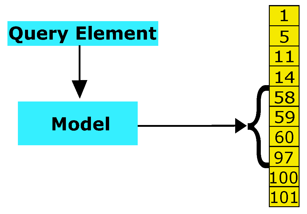
2.2. Learning from Data to Speed Up Sorted Table Search: A Simple View with an Example

Kraska et al. [2] proposed an approach that transforms the Predecessor Search problem into a learning-prediction one. With reference to Figure 1, the model learned from the data is used as a predictor of where a query element may be in the table. To fix ideas, Binary Search is then performed only on the interval returned by the model.

We now outline the simplest technique that can be used to build a model for A and provide an example. It relies on Linear Regression, with Mean Square Error Minimization [52]. We start with the example. Consider Figure 2 and the table A in the caption.

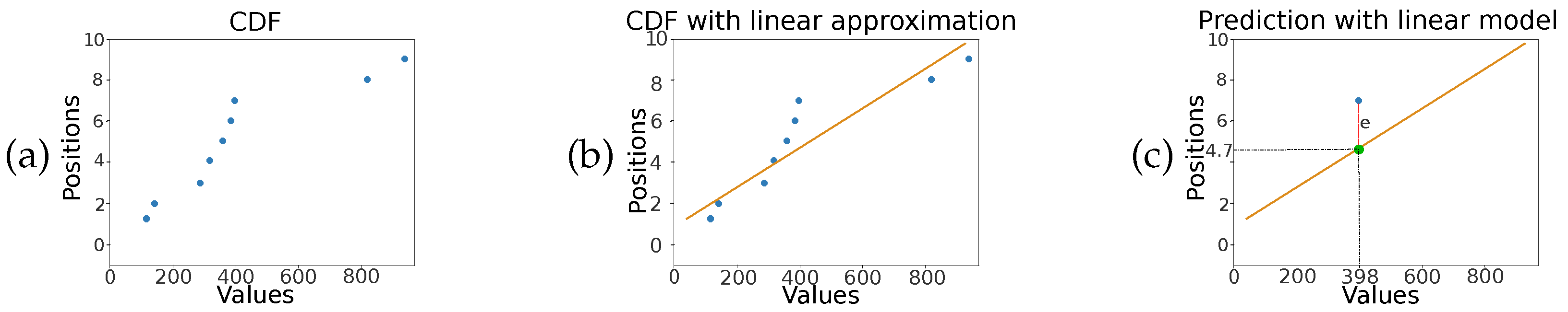
• Ingredient One of Learned Indexing: The Cumulative Distribution Function of a Sorted Table. With reference to Figure 2a, we can plot the elements of A in a graph, where the abscissa reports the value of the elements in the table and the ordinates are their corresponding ranks. The result of the plot is reminiscent of a discrete Cumulative Distribution Function that underlines the table. The specific construction exemplified here can be generalized to any sorted table as discussed in Marcus et al. [9]. In the literature, for a given table, such a discrete curve is referenced as CDF.
• Ingredient Two of Learned Indexing: A Model for theCDF. Now, it is essential to transform the discrete CDF into a continuous curve. The simplest way to do this is to fit a straight line of equation $F\left(x\right)=ax+b$ to the CDF (this process is shown in Figure 2b). In this example, we use Linear Regression with Mean Square Error Minimization in order to obtain a and b. They are 0.01 and 0.85, respectively.
• Ingredient Three of Learned Indexing: The Model Error Correction. Since F is an approximation of the ranks of the elements in the table, in applying it to an element in order to predict its rank, we may produce an error e. With reference to Figure 2c, applying the model to the element 398, we obtain a predicted rank of $4.68$, instead of 7, which is the real rank. Thus, the error made by the model $F\left(x\right)=0.01\times x+0.85$ on this element is $e=7-\lceil 4.68\rceil =2$. Therefore, in order to use the equation F to predict where an element x is in the table, we must correct for this error. Indeed, we consider the maximum error $ϵ$ computed as the maximum distance between the real rank of the elements in the table and the corresponding rank predicted by the model. The maximum error $ϵ$ is used to set the search interval of an element x to be $\left[F\right(x)-ϵ,F(x)+ϵ]$. In the example we are discussing, $ϵ$ is 3.

More in general, in order to perform a query, the model is consulted, and an interval in which to search is returned. Then, Binary Search is performed on that interval. Different models may use different schemes to determine the required range as outlined in Section 2.3. The reader interested in a rigorous presentation of those ideas can consult Marcus et al. [12]. In this paper, we characterize the accuracy in the prediction of a model via the reduction factor: the percentage of the table that is no longer considered for searching after the prediction of a rank.

Regarding the diversity across models to determine the search interval and in order to place all models on par, we empirically estimate the reduction factor of a model. With the use of the model and over a batch of queries, we determine the length of the interval to search into for each query. Based on this, we can immediately compute the reduction factor for that query. Then, we take the average of those reduction factors over the entire set of queries as the reduction factor of the model for the given table.

2.3. A Classification of Learned Indexing Models

With the exception of the Eytzinger Binary Search, all procedures mentioned in Section 2.1 have a natural learned version. Indeed, all models currently known in the literature naturally fit sorted table layouts for the final search stage; however, for that purpose, array layouts other than sorted or more complex data structures cannot be used. Given a learned version of the two mentioned procedures, the time and space performances depend critically on the model used to predict the interval to search into. Here, we propose a classification of models that comprises four classes.

The first two classes, shown in Figure 3, consist of models that use constant space, while the other two, shown in Figure 4, consist of models that use space as a function of some model parameters. For each of them, the reduction factor is determined as described in Section 2. Moreover, as already indicated, the Learned k-ary Search and the Synoptic RMI models are new and fit quite naturally in the classification that we present.

2.3.1. Atomic Models: One Level and No Branching Factor

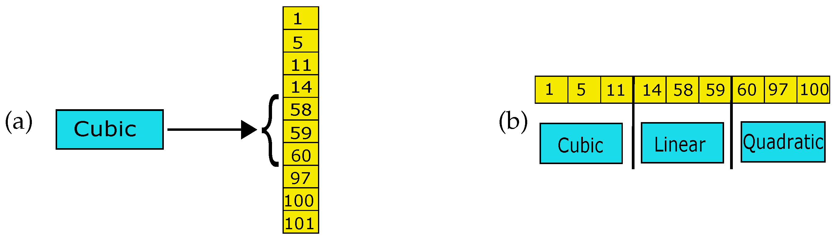
• Simple Regression [52]. We use linear, quadratic and cubic regression models. Each can be thought of as an Atomic Model in the sense that it cannot be divided into “sub-models”. Figure 3a provides an example. We report that the most appropriate regression model in terms of the query times and a reduction factor is the cubic one. We omit those results for brevity and to keep our contribution focused on the important findings. However, they can be found in [51]. For this reason, the cubic model, indicated in the rest of the manuscript by C, is the only one that is included in what follows.

2.3.2. A Two-Level Hybrid Model with a Constant Branching Factor

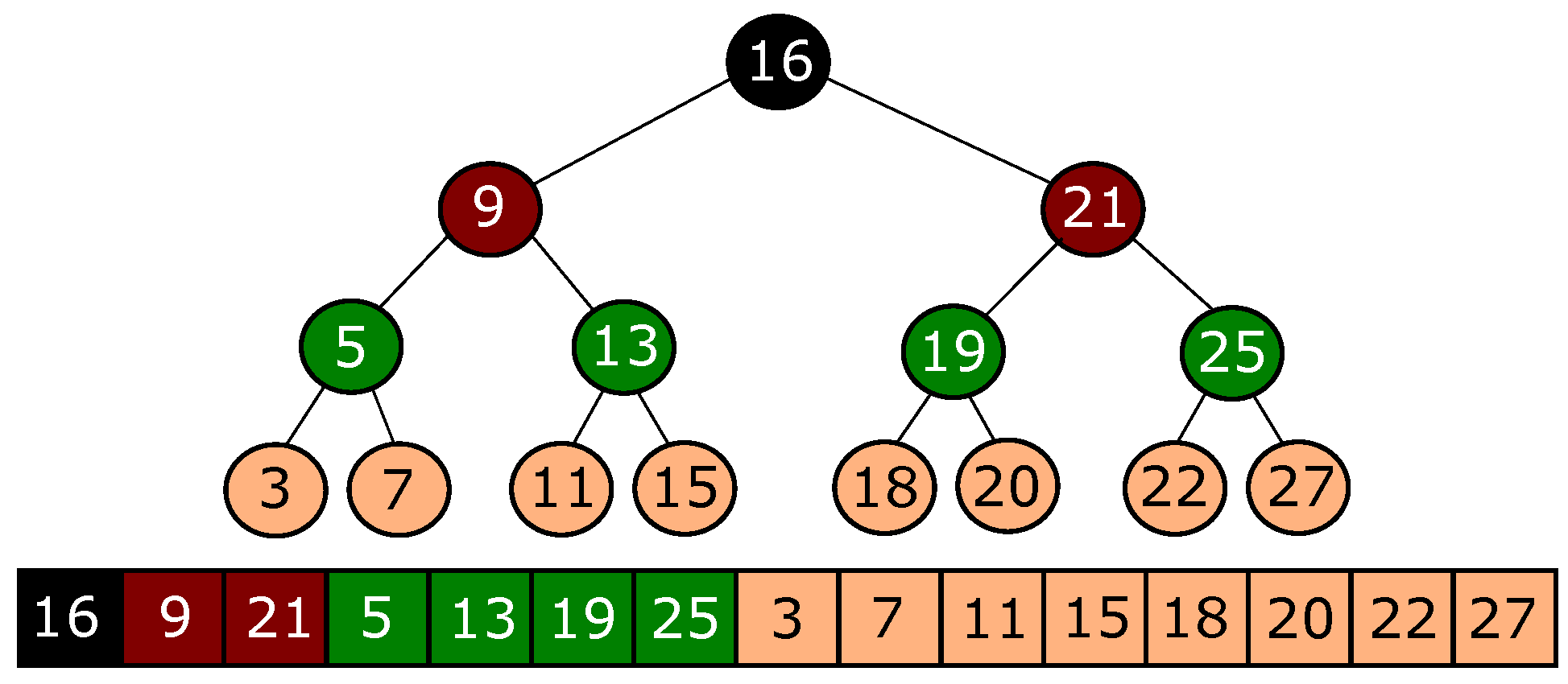
• KO-US: Learned k-ary Search. This model partitions the table into a fixed number of segments, bounded by a small constant, i.e., at most 20 in this study, in analogy with a single iteration of the k-ary Search routine [53,54]. An example is provided in Figure 3b. For each segment, Atomic Models are computed to approximate the CDF of the table elements in that segment. Finally, the model that guarantees the best reduction factor is assigned to each segment. As for the prediction, a sequential search is performed for the second level segment to pick and the corresponding model is used for the prediction, followed by Uniform Binary Search, since it is superior to the Standard one (data not reported and available upon request). We anticipate that, for the experiments conducted in this study, k is chosen in the interval $[3,20]$. For conciseness, only results for the model with $k=15$ are reported, since it is the value with the best performance in terms of query time (data not reported and available upon request). Accordingly, from now on, KO-US indicates the model with $k=15$.

2.3.3. Two-Level RMIs with Parametric Branching Factor

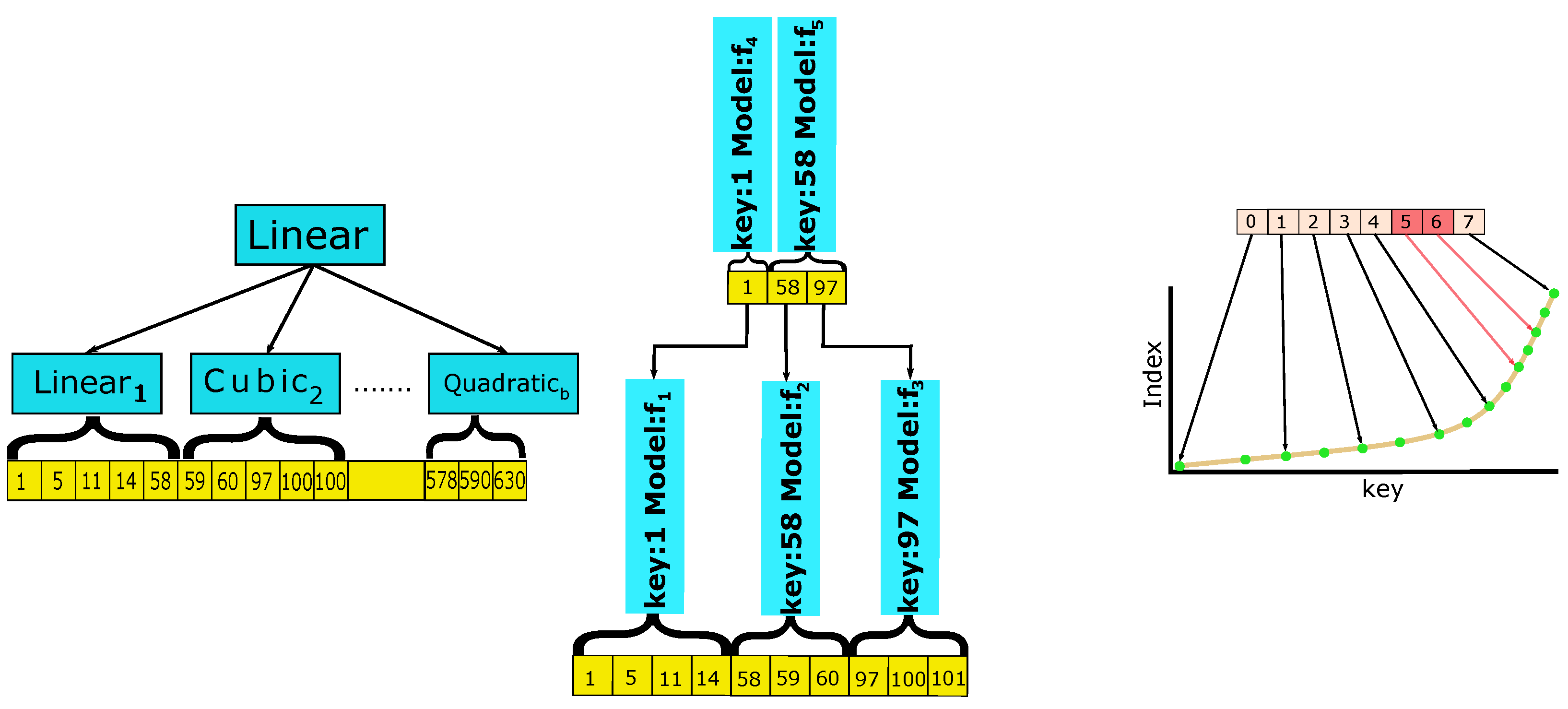
• Heuristically Optimized RMIs. Informally, an RMI is a multi-level, directed graph, with Atomic Models at its nodes. When searching for a given key and starting with the first level, a prediction at each level identifies the model of the next level to use for the next prediction. This process continues until a final level model is reached. This latter is used to predict the table interval to search into. As indicated in the benchmarking study, in most applications, a generic RMI with two layers, a tree-like structure and a branching factor b suffices. An example is provided in Figure 4 on the left. It is to be noted that the Atomic Models are RMIs. Moreover, the difference between Learned k-ary Search and RMIs is that the first level in the former partitions the table, while that same level in the latter partitions the universe of the elements.
  Following the benchmarking study and for a given table, we use two-layer RMIs that we obtain using the optimization software provided in CDFShop, which returns up to ten versions of the generic RMI for a given input table. For each model, the optimization software picks an appropriate branching factor and the type of regression to use within each part of the model—the latter quantities being the parameters that control the precision of its prediction as well as its space occupancy. It is also to be remarked, as indicated in [12], that the optimization process provides only approximations to the real optimum and is heuristic in nature with no theoretic approximation performance guarantees. The problem of finding an optimal model in polynomial time is open.
• SY-RMI: A Synoptic RMI. For a given set of tables of approximately the same size, we use CDFShop as above to obtain a set of models (at most 10 for each table). For the entire set of models thus obtained and each model in it, we compute the ratio (branching factor)/(model space), and we take the median of those ratios as a measure of the branching factor per unit of model space, denoted as $UB$. Among the RMIs returned by CDFShop, we pick the relative majority winner, i.e., the one that provides the best query time, averaged over a set of simulations. When one uses such a model on tables of approximately the same size as the ones used as input to CDFShop, we set the branching factor to be a multiple of $UB$, which depends on how much space the model is expected to use relative to the input table size. This model can be intuitively considered as the one that best summarizes the output of CDFShop in terms of the query time for the given set of tables. The final model is informally referred to as Synoptic.

2.3.4. CDF Approximation-Controlled Models

• PGM [13]. This is also a multi-stage model, built bottom-up and queried top-down. It uses a user-defined approximation parameter $ϵ$, which controls the prediction error at each stage. With reference to Figure 4 in the center, the table is subdivided into three pieces. A prediction in each piece can be provided via a linear model guaranteeing an error of $ϵ$. A new table is formed by selecting the minimum values in each of the three pieces. This new table is possibly again partitioned into pieces, in which a linear model can make a prediction within the given error.
  The process is iterated until only one linear model suffices, as in the case in the figure. A query is processed via a series of predictions, starting at the root of the tree. Furthermore, in this case, for a given table, at most ten models were built as prescribed in the benchmarking study with the use of the parameters, software and methods provided there, i.e, SOSD. It is to be noted that the PGM index, in its bi-criteria version, is able to return the best query time index, within the given amount of space that the model is supposed to use. Experiments are also performed with this version of the PGM, denoted for brevity as B-PGM. The interested reader can find a discussion regarding more variants of this PGM version in [51].
• RS [17]. This is a two-stage model. It also uses a user-defined approximation parameter $ϵ$. With reference to Figure 4 on the right, a spline curve approximating the CDF of the data is built. Then, the radix table is used to identify spline points to use to refine the search interval. Furthermore, in this case, we performed the training as described in the benchmarking study.

In what follows, for ease of reference, models in the first two classes are referred to as constant-space models, while the ones in the remaining classes are parametric-space models.

3. Experimental Methodology

Our experimental setup closely follows the one outlined in the already mentioned benchmarking study by Marcus et al. [9]. Since an intent of this study is to gain deeper insights regarding the circumstances in which learned versions of Sorted Table Search procedure and indexes are profitable in small additional space with respect to the one taken by the input table, across the main memory hierarchy, we derive our own benchmark datasets from the ones in the study by Marcus et al. [9].

3.1. Hardware

All the experiments were performed on a workstation equipped with an Intel Core i7-8700 3.2GHz CPU with three levels of cache memory: (a) 64 kb of L1 cache; (b) 256 kb of L2 cache; and (c) 12 Mb of shared L3 cache. The total amount of system memory is 32 Gbytes of DDR4. The operating system is Ubuntu LTS 20.04.

3.2. Datasets

The same real datasets of the benchmarking study are used. In particular, attention is restricted to integers only, each represented with 64 bits unless otherwise specified. For the convenience of the reader, a list of those datasets, with an outline of their content, is provided next.

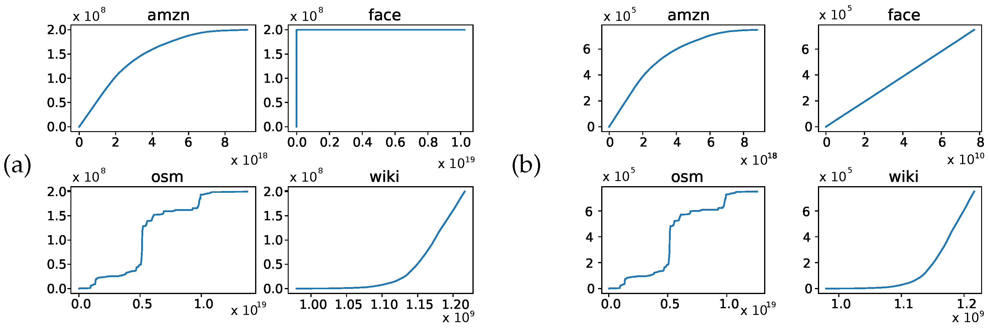
• amzn: book popularity data from Amazon. Each key represents the popularity of a particular book. Although two versions of this dataset, i.e., 32-bit and 64-bit, are used in the benchmarking, no particular differences were observed in the results of our experiments, and, for this reason, we report only those for the 64-bit dataset. The interested reader can find the results for the 32-bit version in [51].
• face: randomly sampled Facebook user IDs. Each key uniquely identifies a user.
• osm: cell IDs from Open Street Map. Each key represents an embedded location.
• wiki: timestamps of edits from Wikipedia. Each key represents the time an edit was committed.

Moreover, for the purpose of this research, as already mentioned above, additional datasets were extracted from the ones just mentioned. For each of those datasets, three new ones were obtained in order to fit each lower level of the internal memory hierarchy. In particular, each new dataset was obtained by sampling the original one so that the CDF was similar to the original one. The interested reader can find more details of this extraction procedure in Appendix A.2. Letting n be the number of elements in a table, for the computer architecture that was used, the details of the generated tables are the following.

• Fitting in L1 cache: cache size 64 Kb. Therefore, $n=3.7K$ was chosen.
• Fitting in L2 cache: cache size 256 Kb. Therefore, $n=31.5K$ was chosen.
• Fitting in L3 cache: cache size 8 Mb. Therefore, $n=750K$ was chosen.
• Fitting in PC main memory (L4): memory size 32 Gb. Therefore, $n=200M$ was chosen, i.e., the entire dataset.

The rationale for the choice of those datasets, in particular the ones coming from the benchmarking study, is that they provide different Empirical CDFs, as shown in Figure 5a, and this allows us to measure the performance of Learned Indexes considering different possible characteristics of real-world data. It is to be noted that the face dataset is somewhat special. Indeed, the shape of its CDF (see Figure 5a) is determined by 21 outliers at the end of the table: all the elements of that dataset, up to the first outlier, have essentially the same distance between consecutive elements—that is, they are all in a straight line.

This regularity breaks with the first outlier that, together with the other ones, does not follow such a nice pattern. For lower memory levels, the CDF of the corresponding face datasets becomes a straight line, as exemplified in Figure 5b for the L3 memory level. As for the remaining datasets, their smaller versions closely follow the CDF of the largest datasets as again exemplified in Figure 5b for the L3 memory level.

As for query dataset generation, for each of the tables built as described above, we extract uniformly and at random (with replacement) from the universe U, a total of two million elements, 50% of which are present and 50% absent, in each table. For coherence, all of the query experiments were performed within SOSD, suitably modified to accommodate all Learned Indexes used in this research. The query time that we report is an average taken on a batch of two million queries executed by a search routine or a Learned Index.

This is essential for Learned Indexes: a measure of a single query performance would be unreliable [55], and in fact SOSD does not allow it, while the method we chose is compliant with the literature [9]. Such a limitation makes it unreliable to measure certain relevant performance parameters of a Learned Index, such as, for each query, the amount of time spent for prediction and the amount of time spent for searching.

In fact, to the best of our knowledge, none of the papers reporting on Learned Indexing provided such a breakdown. Rather they concentrated on the accuracy of the predictions. For completeness, we mention that the query time estimates adopted in the current state of the art and followed here, are accurate—that is, the processing time of a batch of queries is subject to very little standard deviation when averaged over independent executions. Although not perceived as essential in previous work, we provide a highlight of such an assessment using the new and the RMI, PGM and RS models on the amzn datasets. The results are reported in

Table A8. Batch-query time processing over independent executions. The first row indicates the model, while the memory level is indicated by the first column. Each entry in the table indicates the average time (in seconds) to execute 10 times the same batch of queries together with the corresponding standard deviation.

	RMI	PGM	RS	SY-RMI 0.05	KO-US
L1	$2.35\times {10}^{-2}\pm 5.56\times {10}^{-4}$	$3.27\times {10}^{-2}\pm 1.49\times {10}^{-3}$	$2.61\times {10}^{-2}\pm 3.69\times {10}^{-4}$	$2.34\times {10}^{-2}\pm 3.69\times {10}^{-4}$	$2.90\times {10}^{-1}\pm 1.1\times {10}^{-2}$
L2	$3.02\times {10}^{-2}\pm 4.20\times {10}^{-4}$	$3.88\times {10}^{-2}\pm 9.93\times {10}^{-4}$	$3.44\times {10}^{-2}\pm 2.89\times {10}^{-4}$	$3.02\times {10}^{-2}\pm 4.20\times {10}^{-4}$	$2.99\times {10}^{-1}\pm 8.04\times {10}^{-3}$
L3	$6.78\times {10}^{-2}\pm 1.02\times {10}^{-3}$	$7.16\times {10}^{-2}\pm 1.31\times {10}^{-3}$	$8.33\times {10}^{-2}\pm 1.40\times {10}^{-3}$	$6.78\times {10}^{-2}\pm 1.02\times {10}^{-3}$	$3.81\times {10}^{-1}\pm 1.09\times {10}^{-2}$
L4	$1.66\times {10}^{-1}\pm 3.93\times {10}^{-3}$	$1.67\times {10}^{-1}\pm 1.90\times {10}^{-3}$	$1.62\times {10}^{-1}\pm 1.53\times {10}^{-3}$	$1.66\times {10}^{-1}\pm 3.94\times {10}^{-3}$	$7.37\times {10}^{-1}\pm 5.40\times {10}^{-3}$

of Appendix A.4. Finally, in terms of theoretic worst-case analysis, the prediction for the RMIs used here takes $O\left(1\right)$ time and $O\left(logn\right)$ time for the PGM and the RS.

4. Training of the Novel Models: Analysis and Insights into Model Training

We now focus on the training phase of the novel models, and we compare their performance with the literature standards included in this research. In order to assess how well a Learned Index model can be trained, three indicators are important: the time required for learning, the reduction factor that one obtains and the time needed to perform the prediction. A quantification of the first parameter is provided and discussed here. The other two indicators are strongly dependent on each other, with the reduction factor being related to space. In turn, those two indicators affect the query time. Therefore, they are best discussed in Section 5. We anticipate that our analysis of the training time performed here provides useful and novel insights into model training for Learned Indexing. All the training experiments were performed on the datasets mentioned in Section 3.2 across all internal memory levels.

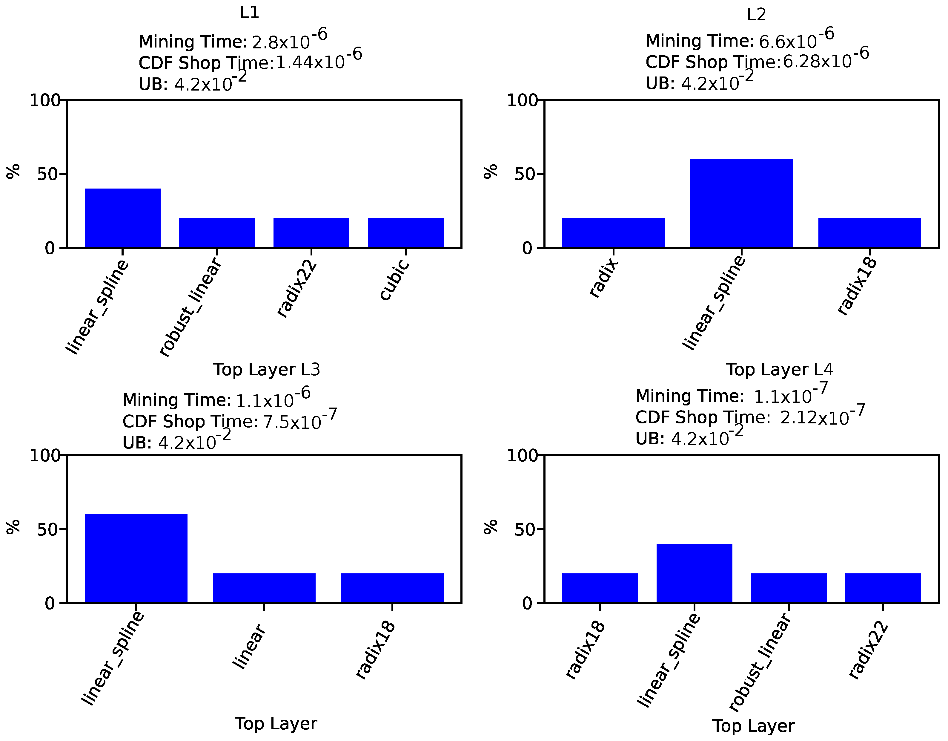
4.1. Mining SOSD Output for the Synoptic RMI

As anticipated in Section 2.3, in order to set the levels and $UB$ of the Synoptic RMI, it is necessary to process the output of SOSD for each dataset and memory level. Indeed, as described in Section 2.3, once we set a space budget for the model, the corresponding branching factor was computed by multiplying it by $UB$. In particular, we computed three versions of a Synoptic RMI using a percentage of space of 0.05%, 0.7% and 2% with respect to the input table size.

With regard to the layers choice, the simulation to identify the relative majority RMIs was performed on query datasets extracted as described in the previous Section but using only $1\%$ of the number of query elements specified there. The statistics regarding the results of such a simulation are summarized in Figure 6. In particular, for each memory level, we report the computed $UB$. Furthermore, limited to the top layer of an RMI, we also report the models associated with the best ones. The time it took to identify the proper Synoptic RMI (average time per element, over all the RMIs returned by CDFShop, denoted as the mining time) is also reported, together with the same time required to obtain the output of CDFShop.

As is evident, the mining time is comparable with the performance of CDFShop. It is also evident from that figure that the variety of best-performing models represents various challenges for the learning of the CDF of real datasets. Therefore, given such a variety, it is far from obvious that the median $UB$ is the same for each memory level. Moreover, the relative majority model is also the same across memory levels, i.e., linear spline, with linear models for each segment of the second layer.

4.2. Training Time Comparison between Novel Models and the State of the Art

In what follows, we divide the training-time comparison into two groups: constant- and parametric-space models. For the first group, we consider the new model and only the Cubic Atomic Model, excluding the linear and quadratic ones for the reasons mentioned earlier in this paper. For the Cubic Model, the training time on a given dataset is due to the computation of its parameters via polynomial regression. As for the Learned k-ary Search Model, its training consists of partitioning the table into k segments. Then, for each segment, Atomic Models are used to approximate the local CDF of the elements belonging to that segment, and, among them, the model with the best reduction factor is chosen.

For each dataset and each memory level, the resulting training times are reported in

Table 1. Constant-space model training time for the L4 tables. The first column indicates the datasets. The remaining columns indicate the model used for the learning phase. Each entry reports the training time in seconds and per element.

	KO-US	C
amzn	$3.7\times {10}^{-8}$	$1.4\times {10}^{-8}$
face	$3.6\times {10}^{-8}$	$1.4\times {10}^{-8}$
osm	$3.6\times {10}^{-8}$	$1.4\times {10}^{-8}$
wiki	$3.6\times {10}^{-8}$	$1.4\times {10}^{-8}$

and

Table A2. Constant-space model training time for L1 Tables. The first column indicates the datasets. The remaining columns indicate the models used for the learning phase. Each entry reports the training time in seconds and per element.

	KO-US	C
amzn	$5.3\times {10}^{-7}$	$1.0\times {10}^{-7}$
face	$5.5\times {10}^{-7}$	$8.5\times {10}^{-8}$
osm	$4.6\times {10}^{-7}$	$9.9\times {10}^{-8}$
wiki	$9.0\times {10}^{-7}$	$7.9\times {10}^{-8}$

,

Table A3. Constant-space model training time for L2 Tables. The table legend is as in Table A2.

	KO-BFS	C
amzn	$1.8\times {10}^{-7}$	$3.1\times {10}^{-7}$
face	$1.0\times {10}^{-7}$	$2.8\times {10}^{-7}$
osm	$1.2\times {10}^{-7}$	$2.9\times {10}^{-7}$
wiki	$1.0\times {10}^{-7}$	$2.7\times {10}^{-7}$

and

Table A4. Constant-space model training time for L3 Tables. The table legend is as in Table A2.

	KO-US	C
amzn	$6.3\times {10}^{-8}$	$1.9\times {10}^{-8}$
face	$3.9\times {10}^{-8}$	$1.9\times {10}^{-8}$
osm	$4.4\times {10}^{-8}$	$2.0\times {10}^{-8}$
wiki	$4.1\times {10}^{-8}$	$1.9\times {10}^{-8}$

of Appendix A.3. As expected, the Learned k-ary Search Model is slower than the Cubic Atomic Model; however, the important fact is that the slowdown is due to constant multiplicative factors rather than being of an order of magnitude—that is, the slow-down is tolerable. Another additional and counter-intuitive finding is that the training time of both models, on average, is better for the cases of large datasets with respect to smaller ones. We analyzed the training code in order to obtain insight into such a fact. We found that the cost of the matrix products involved in the training computation of both models depends on the size of the involved operands. As the size of the dataset grows, such a cost is amortized on a larger and larger number of elements.

Regarding the second group, we consider the new model and the ones described in Section 2.3, i.e., RMI, PGM and RS. The training time was computed using two different platforms: CDFShop in the case of the Synoptic RMI and RMI as well as SOSD for PGM and RS. It is useful to recall that, in the case of the state-of-the-art models, the result of a single execution of those two platforms returns a batch of up to ten models, and thus the reported times refer to the execution of the entire learning suite—that is, the training of those models consists of a batch of model instances from which a user can choose.

On the other hand, for the Synoptic RMI, this refers to the training of a single RMI with a given branching factor and layer composition. For each dataset and each memory level, the results are reported in

Table 2. Parametric-model training time for the L4 tables. The first column indicates the datasets. The remaining columns indicate the model used for the learning phase. In particular, each entry reports the time to train the Synoptic RMI and an entire batch of models via the CDFShop and the SOSD libraries as specified in the main text. The time is in seconds and per element.

	CDFShop SY-RMI 2%	CDFShop RMI	SOSD RS	SOSD PGM
amzn	$1.1\times {10}^{-6}$	$2.2\times {10}^{-6}$	$2.1\times {10}^{-7}$	$5.0\times {10}^{-7}$
face	$1.3\times {10}^{-6}$	$2.5\times {10}^{-6}$	$2.1\times {10}^{-7}$	$6.5\times {10}^{-7}$
osm	$1.2\times {10}^{-6}$	$2.5\times {10}^{-6}$	$2.2\times {10}^{-7}$	$7.4\times {10}^{-6}$
wiki	$1.1\times {10}^{-6}$	$2.2\times {10}^{-6}$	$1.9\times {10}^{-7}$	$4.1\times {10}^{-7}$

and

Table A5. Parametric-space model training time for L1 Tables. The first column indicates the datasets. The remaining columns indicate the models used for the learning phase. In particular, each entry reports the time used by the CDFShop and SOSD libraries to train the entire batch of parametric models in seconds and per element.

	CDFShop SY-RMI 2%	CDFShop RMI	SOSD RS	SOSD PGM
amzn	$5.2\times {10}^{-6}$	$5.6\times {10}^{-6}$	$3.5\times {10}^{-6}$	$5.0\times {10}^{-7}$
face	$4.1\times {10}^{-6}$	$4.6\times {10}^{-6}$	$1.1\times {10}^{-6}$	$3.9\times {10}^{-7}$
osm	$2.8\times {10}^{-4}$	$2.9\times {10}^{-4}$	$6.9\times {10}^{-6}$	$4.0\times {10}^{-7}$
wiki	$7.8\times {10}^{-6}$	$9.3\times {10}^{-6}$	$1.0\times {10}^{-5}$	$3.7\times {10}^{-7}$

,

Table A6. Parametric-space model training time for L2 Tables. The table legend is as in Table A5.

	CDFShop SY-RMI 2%	CDFShop RMI	SOSD RS	SOSD PGM
amzn	$5.2\times {10}^{-6}$	$5.6\times {10}^{-7}$	$3.5\times {10}^{-7}$	$5.0\times {10}^{-8}$
face	$4.1\times {10}^{-6}$	$4.6\times {10}^{-7}$	$1.1\times {10}^{-7}$	$3.9\times {10}^{-8}$
osm	$2.8\times {10}^{-4}$	$2.9\times {10}^{-5}$	$6.9\times {10}^{-7}$	$4.0\times {10}^{-8}$
wiki	$7.8\times {10}^{-6}$	$9.3\times {10}^{-7}$	$1.0\times {10}^{-6}$	$3.7\times {10}^{-8}$

and

Table A7. Parametric-space model training time for L3 Tables. The table legend is as in Table A5.

	CDFShop SY-RMI 2%	CDFShop RMI	SOSD RS	SOSD PGM
amzn	$1.5\times {10}^{-6}$	$1.3\times {10}^{-7}$	$2.4\times {10}^{-8}$	$3.4\times {10}^{-8}$
face	$1.5\times {10}^{-5}$	$1.6\times {10}^{-6}$	$1.4\times {10}^{-8}$	$2.4\times {10}^{-8}$
osm	$1.2\times {10}^{-5}$	$1.3\times {10}^{-6}$	$3.5\times {10}^{-8}$	$3.8\times {10}^{-8}$
wiki	$2.3\times {10}^{-6}$	$2.2\times {10}^{-7}$	$5.1\times {10}^{-8}$	$3.7\times {10}^{-8}$

of Appendix A.3. The time needed to train the Synoptic RMI is comparable to the one needed to train a batch of RMI models. This latter, as already known, is worse than the time to train a batch of RS or PGM models. Such results are not considered problematic for the deployment of the RMI in application contexts, and the training time of the Synoptic RMI is in-line with the mentioned literature standards. For completeness, we mention that the reason for which the time needed to train a unique Synoptic RMI model is very close to the training of a batch on RMI models is due to the library start-up overhead time.

Such a time is mitigated for the case of the training of a batch of models, while it becomes dominant in training a single model. Fortunately, the CDFShop or the SOSD training executions are a “one-time-only” processes, in which the output can then be reused over and over again, suggesting that this overhead time is of little relevance for the case of a production environment.

4.3. Insights into the Training Time of the RS and PGM Models

Another important contribution that this research provides is a more refined assessment of the relation between the RS and PGM indexes, in terms of the training time. In

Table 3. Comparison between the RS and PGM training times. For each dataset and memory level, we report the training times for the RS and PGM models in seconds. Panel (a) refers to memory levels L1 and L2, while Panel (b) refers to L3 and L4.

Panel (a)
	L1		L2
	SOSD RS	SOSD PGM	SOSD RS	SOSD PGM
amzn	$3.5\times {10}^{-6}$	$5.0\times {10}^{-7}$	$3.5\times {10}^{-7}$	$5.0\times {10}^{-8}$
face	$1.1\times {10}^{-6}$	$3.9\times {10}^{-7}$	$1.1\times {10}^{-7}$	$3.9\times {10}^{-8}$
osm	$6.9\times {10}^{-6}$	$4.0\times {10}^{-7}$	$6.9\times {10}^{-7}$	$4.0\times {10}^{-8}$
wiki	$1.0\times {10}^{-5}$	$3.7\times {10}^{-7}$	$1.0\times {10}^{-6}$	$3.7\times {10}^{-8}$
Panel (b)
	L3		L4
	SOSD RS	SOSD PGM	SOSD RS	SOSD PGM
amzn	$2.4\times {10}^{-8}$	$3.4\times {10}^{-8}$	$2.1\times {10}^{-7}$	$5.0\times {10}^{-7}$
face	$1.4\times {10}^{-8}$	$2.4\times {10}^{-8}$	$2.1\times {10}^{-7}$	$6.5\times {10}^{-7}$
osm	$3.5\times {10}^{-8}$	$3.8\times {10}^{-8}$	$2.2\times {10}^{-7}$	$7.4\times {10}^{-7}$
wiki	$5.1\times {10}^{-8}$	$3.7\times {10}^{-8}$	$1.9\times {10}^{-7}$	$4.1\times {10}^{-7}$

, for each dataset and memory level, we report the training times of those two indexes. As discussed in [17], those two Learned Indexes can both be built in one pass over the input with important implications: one being that they can be trained faster than the RMIs—even one order of magnitude sped up. However, in that study as well as in the benchmarking one, the RS was reported as superior to the PGM in terms of the training time.

It is to be noted that the datasets that they used are the largest ones in this study. With reference to Table 3, our experiments confirm such a finding. On the other hand, the PGM is more effective in terms of the training time across the lower memory hierarchy. The reason may be the following. Those two indexes both use streaming procedures in order to approximate the CDF of the input dataset within a parameter $ϵ$ via the use of straight-line segments that partition the universe. The main difference between the two is that the latter finds an optimal partition, determined via a well-known algorithm (see references in [13]), while the former finds a partition that approximates the optimal as described in [18]. Such an approximation algorithm is supposed to be faster than the optimal one; however, apparently, this speed pays off on large datasets.

5. Query Experiments

The query experiments were performed using all the methods described in Section 2.1 and Section 2.3. The query datasets were generated as described in Section 3.2, and the models were trained as described in Section 4. Following that section, we divided the presentation of the query experiments and the relative discussion into two groups. For both groups, for conciseness, we report here only the experiments for the amzn and the osm datasets since they are representative of two different levels of difficulty in learning their CDFs. The results regarding the other datasets are reported in Appendix A.5.

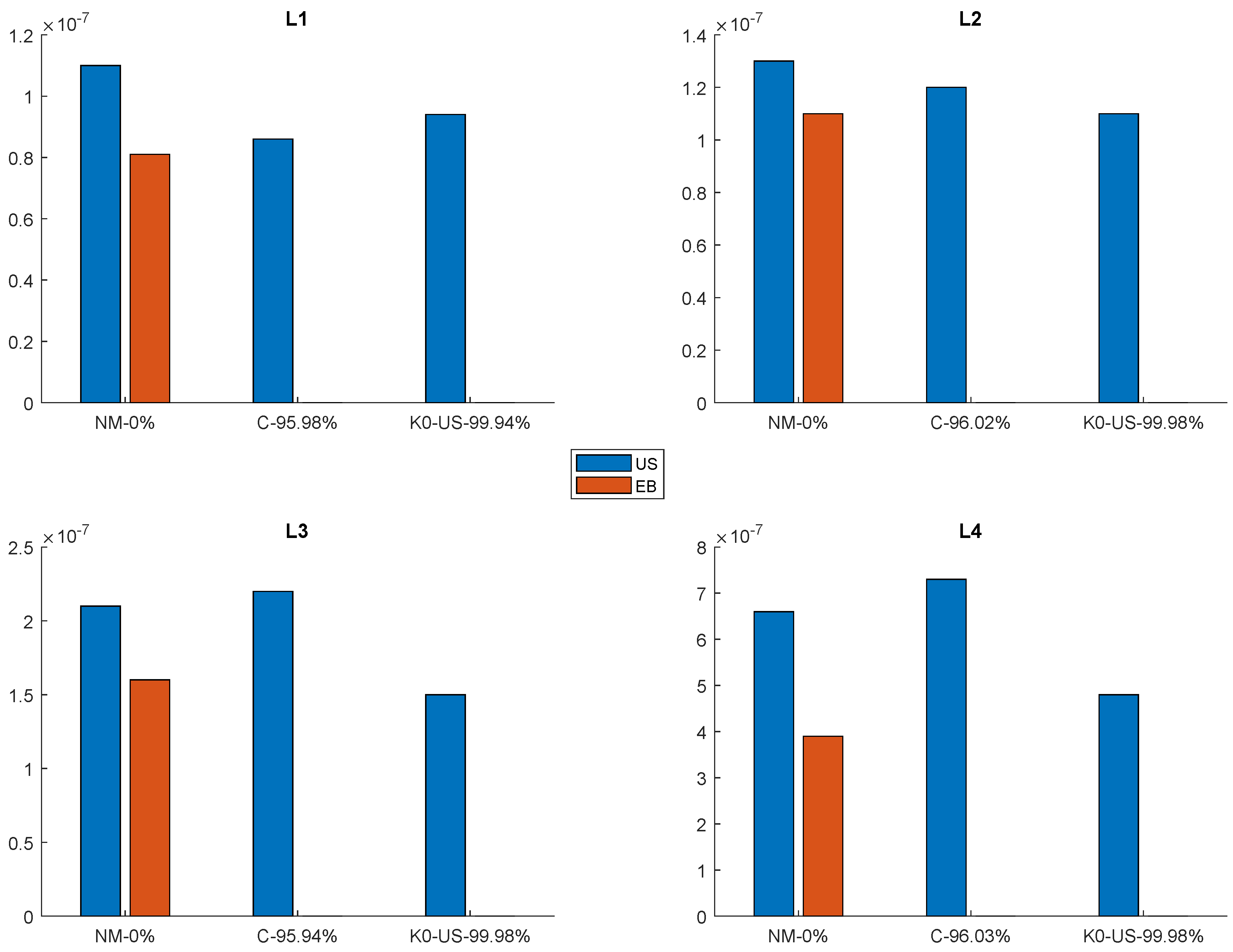
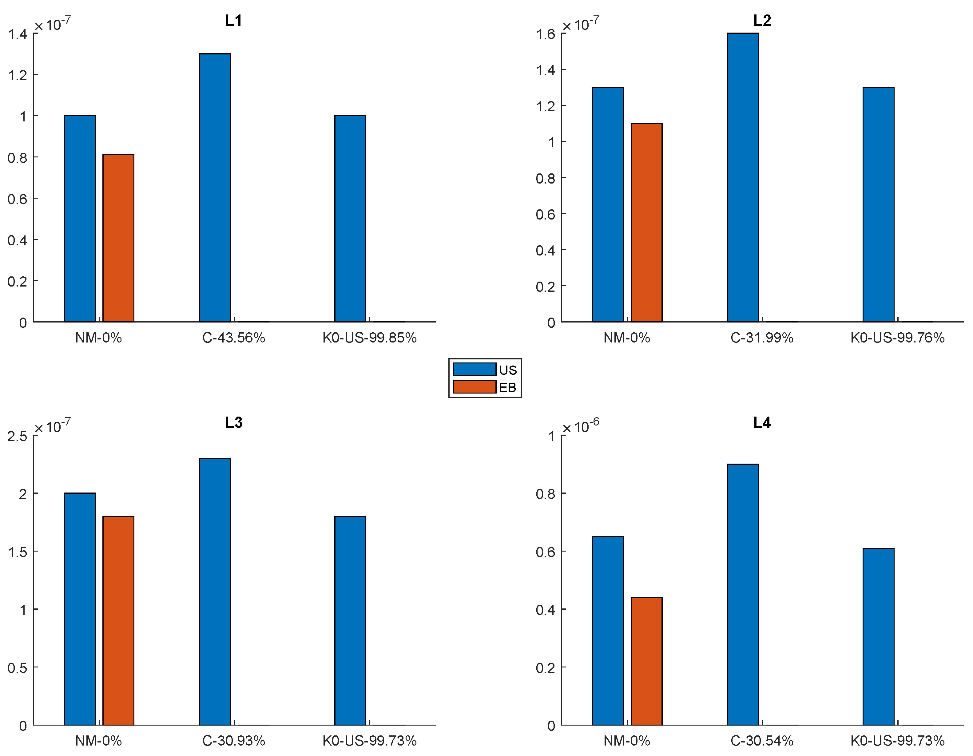
5.1. Constant-Space Models

The results of the experiments for this group of models are reported in Figure 7 and Figure 8 for the amzn and the osm datasets, respectively, and in Figure A2 and Figure A3 of the Appendix A.5, for the remaining ones. In those figures, only the query time for Uniform Binary Search is reported, since the results are analogous to the ones obtained by using the Standard routine. In addition, the query time for the Eytzinger Binary Search is also reported as a useful baseline due to its superiority among the classic routines that take constant additional space with respect to the size of the input table as discussed in [23]. From the mentioned figures, it is evident that the query performance of each model considered here is highly influenced by how difficult to learn the CDF of the input table is as explained next.

• The Cubic Model achieved a high reduction factor, i.e., $\approx 99\%$, on the versions of the face dataset for the first three levels of the internal memory hierarchy, and it was also the best performing, even compared to the Eytzinger Layout routine. This is a quite remarkable achievement; however, the involved datasets had an almost uniform CDF, while a few outliers disrupt this uniformity on the L4 version of that dataset (see Figure 5 and the discussion regarding the face dataset in Section 3.2).
• The Learned k-ary Search Model achieved a high reduction factor on all versions of the amzn and the wiki datasets, i.e., $\approx 99.73$ and was faster than the Uniform Binary Search and the Cubic Model. Those datasets have a regular CDF across all the internal memory levels. It is to be noted that the Eytzinger Layout routine is competitive with the Learned k-ary Search Model.
• No constant space Learned Model won on the difficult-to-learn dataset. The osm dataset has a difficult-to-learn CDF (see Figure 5), and such a characteristic is preserved across the internal memory levels. The Learned k-ary Search Model achieved a respectable reduction factor, i.e., $\approx 98\%$, but no speed increase with respect to Uniform Binary Search. In order to obtain insights into such a counter-intuitive behavior, we performed an additional experiment.
  For each representative dataset and as far as the Learned k-ary Search Model is concerned, we computed two kinds of reduction factors: the first was the global one, achieved considering the size of the entire table, while the second was the local one, computed as the average among the reduction factors of each segment. Those results are reported in

  Table 4. Global and local reduction factors. For the two representative datasets, i.e., amzn and osm, and for each memory level, in each entry, we report the global reduction factor (left) and the local one (right).

  	amzn	osm
  L1	99.94−99.48	98.12−86.70
  L2	99.98−99.56	98.07−86.57
  L3	99.98−99.53	97.98−86.43
  L4	99.98−99.54	98.03−86.57

  . For the osm dataset, it is evident that the local reduction factors are consistently lower than the global ones, highlighting that its CDF is also locally difficult to approximate, which, in turn, implies an ineffective use of the local prediction for the Learned k-ary Search, resulting in poor time performance. Finally, it is to be noted that the Eytzinger Layout routine was the best performing.

In conclusion, in applications where there is a constant space constraint with respect to the input table and where a layout other than sorted can be used, then the Eytzinger Binary Search is still the best choice unless the CDF of the input dataset is particularly easy to approximate. If such a layout cannot be afforded, the best choice is the use of a constant-space model, in particular the Learned k-ary Search Model only for datasets with a CDF that is simple to approximate, otherwise the use of Uniform Binary Search alone is indicated.

Our research extends the results in [23] regarding the Eytzinger Binary Search routine: even compared to Learned Indexes that use constant space, it still results as competitive and many times superior to the others.

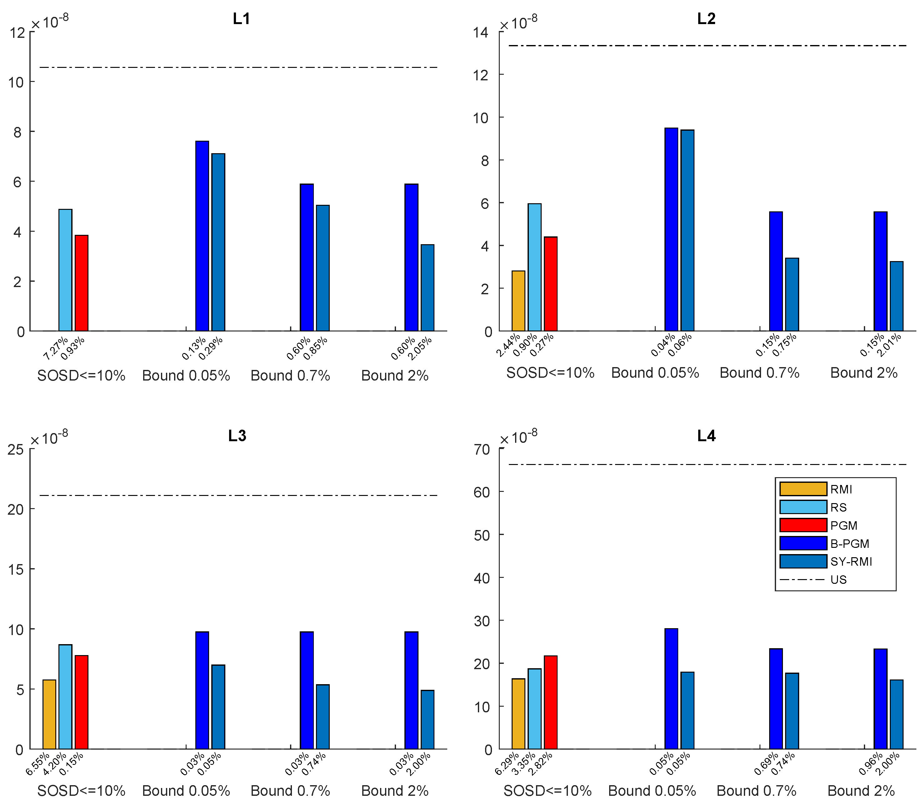
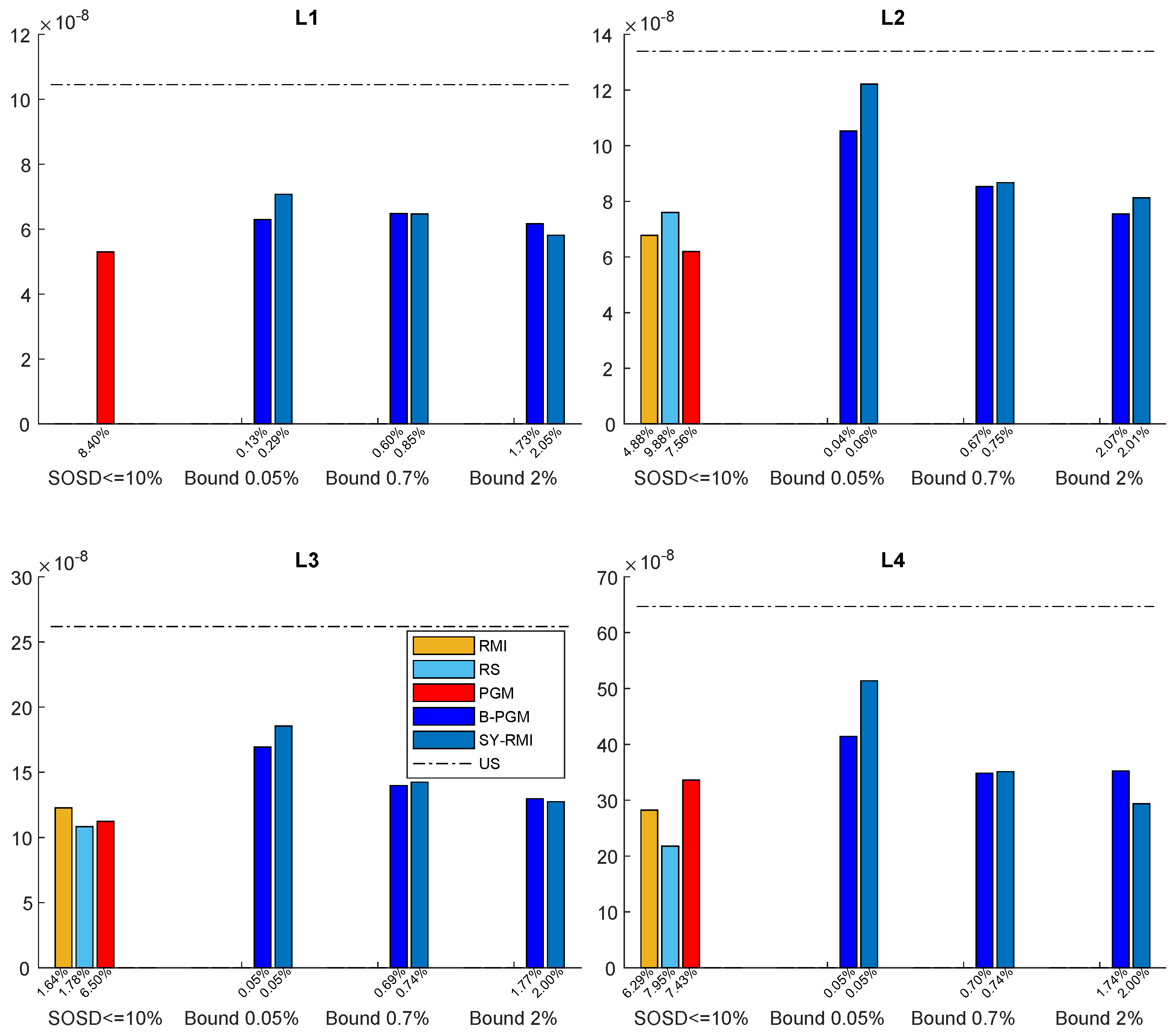
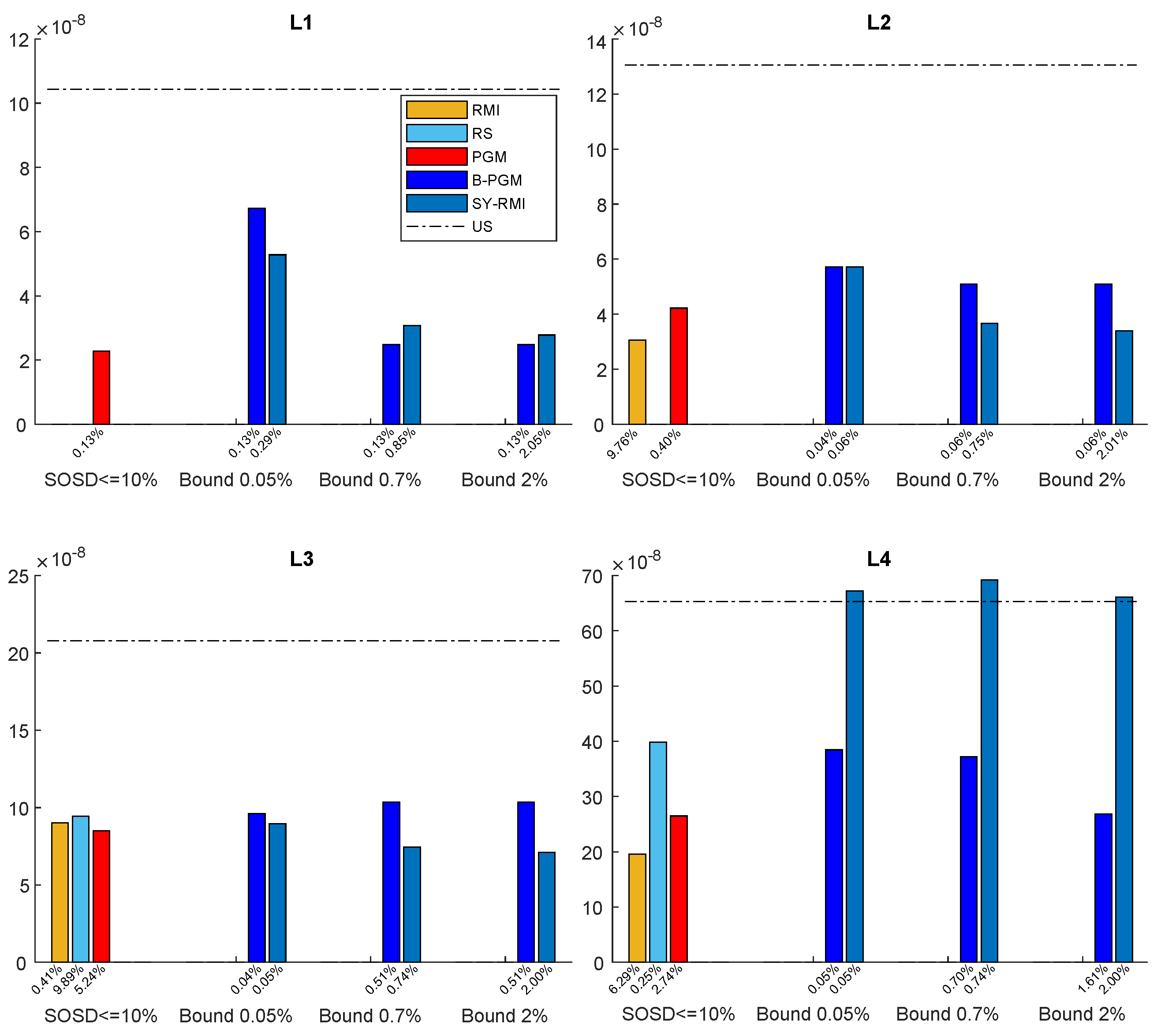
5.2. Parametric-Space Models

For the convenience of the reader, we recall that the model classes involved are: RMI, RS, PGM, the Synoptic RMI and the bi-criteria PGM, which are trained on the input datasets (see Section 3.2) as reported in Section 4. The batch of queries used here was obtained as described in Section 3.2 and, for the query time, we took the average per element as specified in that section. For each of the first three model classes, we considered, among the trained models, the fastest in terms of the query time and those taking less than $10\%$ of space with respect to the the space taken by the input table.

For the other two model classes, we considered three increasing bounds on space, i.e., $0.05\%$, $0.7\%$ and $2\%$, with respect to the space of the table alone. Moreover, as a measure of the Learned Indexes speed up, we also report the query time of the Uniform Binary Search. The results of the corresponding experiments are reported in Figure 9 and Figure 10 for the amzn and osm datasets, respectively, and in Figure A4 and Figure A5 of the Appendix A.5 for the remaining ones.

An interesting finding is that both the Synoptic RMI and the bi-criteria PGM performed better than Uniform Binary Search across datasets and memory levels using very little additional space—that is, one can enjoy the speed of Learned Indexes with a very small space penalty. Moreover, it is important to note that, except for the L1 memory level, the space of those two models is very close to the user-defined bound. Furthermore, in terms of query performances, such two models seem to be complementary. In fact, the bi-criteria PGM performed better on the L1 and L4 memory levels, while the Synoptic RMI performed better on the remaining ones. This complementary and effective control of space makes these two models quite useful in practice.

In addition to those findings, our research provides some more insights into the time–space relation in Learned Indexes, thereby, extending the results of the benchmark study as we now discuss.

• Space Constraints and the Models Provided by SOSD. We fixed a rather small space budget, i.e., at most $10\%$ of additional space in order for a model returned by SOSD to be considered. The RS Index was not competitive with respect to the other Learned Indexes. Those latter consistently use less space and time across datasets and memory levels. As for the RMIs coming out of SOSD, they were not able to operate in a small space at the L1 memory level. On the other memory levels, they were competitive with respect to the bi-criteria PGM and the Synoptic RMI; however, they required more space with respect to them.
• Space, Time and Accuracy of Models. As stated in the benchmarking study, a common view of Learned Indexing Data Structures is as a CDF lossy compressor; see also [2,13]. In this view, the quality of a Learned Index can be judged by the size of the structure and its reduction factor. In that study, it was also argued that this view does not provide an accurate selection criterion for Learned Indexes. Indeed, it may very well be that an index structure with an excellent reduction factor takes a long time to produce a search bound, while an index structure with a worse reduction factor that quickly generates an accurate search bound may be of better use. In the benchmarking study, they also provided evidence that the space–time trade-off is the key factor in determining which model to choose.
  Our contribution is to provide additional results supporting those findings. To this end, we conducted several experiments, whose results are reported in

  Table 5. A synoptic table of space, time and accuracy of the models on the amzn dataset. For each memory level, we report, in the first row, the best performing method for that memory level. The columns named time, space and reduction factor indicate, for this best model, the average query time in seconds, the average additional space used in Kb and the average of the empirical reduction factor. In the second row, we report the versions of the RMI, RS, PGM and Synoptic RMI models that use the least space. In particular, the number next to the models represents, in percentage, the bound on the used space with respect to the input dataset. The columns indicate the ratio of the model/best model of the time, space and reduction factor.

  L1
  	Time	Space	Reduction Factor
  Best RMI	$1.89\times {10}^{-8}$	$3.09$	$99.84$
  B-PGM 0.05	$4.03$	$1.30\times {10}^{-2}$	$2.50\times {10}^{-1}$
  SY-RMI 0.05	$3.77$	$2.85\times {10}^{-2}$	$1.75\times {10}^{-1}$
  RS < 10	$2.58$	$7.06\times {10}^{-1}$	$9.29\times {10}^{-1}$
  Best RMI	$1.00$	$1.00$	$1.00$
  L2
  	Time	Space	Reduction Factor
  Best RMI	$2.51\times {10}^{-8}$	$6.16$	$99.97$
  B-PGM 0.05	$3.78$	$1.62\times {10}^{-2}$	$9.16\times {10}^{-1}$
  SY-RMI 0.05	$3.74$	$2.60\times {10}^{-2}$	$6.44\times {10}^{-1}$
  Best RS < 10	$2.38$	$3.68\times {10}^{-1}$	$9.92\times {10}^{-1}$
  Best RMI	$1.00$	$1.00$	$1.00$
  L3
  	Time	Space	Reduction Factor
  Best RMI	$4.70\times {10}^{-8}$	$6.29\times {10}^3$	$100.00$
  B-PGM 0.05	$2.07$	$3.05\times {10}^{-4}$	$1.00$
  SY-RMI 0.05	$1.49$	$4.79\times {10}^{-4}$	$9.99\times {10}^{-1}$
  RS < 10	$1.59$	$4.00\times {10}^{-2}$	$1.00$
  RMI < 10	$1.03$	$6.25\times {10}^{-2}$	$1.00$
  L4
  	Time	Space	Reduction Factor
  Best RMI	$1.51\times {10}^{-7}$	$2.01\times {10}^5$	$100.00$
  B-PGM 0.05	$1.85$	$3.93\times {10}^{-3}$	$1.00$
  SY-RMI 0.05	$1.18$	$3.97\times {10}^{-3}$	$1.00$
  Best RS	$1.19$	$7.16\times {10}^{-2}$	$1.00$
  RMI < 10	$1.03$	$5.00\times {10}^{-1}$	$1.00$

  and

  Table 6. A synoptic table of space, time and accuracy of the models on the osm dataset. The legend is as in Table 5.

  L1
  	Time	Space	Reduction Factor
  Best RMI	$2.72\times {10}^{-8}$	$1.15\times {10}^3$	$99.87$
  B-PGM 0.05	$2.31$	$3.49\times {10}^{-5}$	$1.74\times {10}^{-1}$
  SY-RMI 0.05	$2.60$	$7.67\times {10}^{-5}$	$2.30\times {10}^{-1}$
  Best RMI	$1.00$	$1.00$	$1.00$
  Best RS	$1.19$	$4.33\times 10$	$9.99\times {10}^{-1}$
  L2
  	Time	Space	Reduction Factor
  Best RMI	$3.93\times {10}^{-8}$	$1.84\times {10}^3$	$99.97$
  B-PGM 0.05	$2.68$	$5.45\times {10}^{-5}$	$7.75\times {10}^{-1}$
  SY-RMI 0.05	$3.11$	$8.72\times {10}^{-5}$	$7.24\times {10}^{-1}$
  RMI < 10	$1.73$	$6.71\times {10}^{-3}$	$9.87\times {10}^{-1}$
  RS < 10	$1.93$	$1.36\times {10}^{-2}$	$9.79\times {10}^{-1}$
  L3
  	Time	Space	Reduction Factor
  Best RS	$7.06\times {10}^{-8}$	$4.63\times {10}^4$	$100.00$
  B-PGM 0.05	$2.40$	$6.22\times {10}^{-5}$	$9.98\times {10}^{-1}$
  SY-RMI 0.05	$2.63$	$6.52\times {10}^{-5}$	$9.31\times {10}^{-1}$
  RMI < 10	$1.75$	$2.12\times {10}^{-3}$	$9.97\times {10}^{-1}$
  RS < 10	$1.55$	$2.31\times {10}^{-3}$	$1.00$
  L4
  	Time	Space	Reduction Factor
  Best RS	$2.04\times {10}^{-7}$	$5.08\times {10}^5$	$100.00$
  SY-RMI 0.05	$2.52$	$1.57\times {10}^{-3}$	$9.99\times {10}^{-1}$
  B-PGM 0.05	$2.03$	$1.59\times {10}^{-3}$	$1.00$
  RMI < 10	$1.18$	$1.98\times {10}^{-1}$	$1.00$
  RS < 10	$1.05$	$2.50\times {10}^{-1}$	$1.00$

  and

  Table A9. A synoptic table of space, time and accuracy of the models on the face dataset. For each memory level, we report, in the first row, the best performing method for that memory level. The columns named time, space and reduction factor indicate, for this best model, the average query time in seconds, the average additional space used and the average of the empirical reduction factor. From the second row, we report the versions of the RMI, RS, PGM and Synoptic RMI models that use the least space. In particular, the numbers next to the models represent the percentage of the used space with respect to the input dataset. The columns indicate the ratio of the model/best model of the time, space and reduction factor.

  L1
  	Time	Space	Reduction Factor
  Best PGM	$2.26\times {10}^{-8}$	$4.00\times {10}^{-2}$	99.52
  Best PGM	1.00	1.00	1.00
  SY-RMI 0.05	2.33	2.20	$6.30\times {10}^{-1}$
  Best RMI	1.16	$7.72\times {10}^1$	1.00
  Best RS	1.17	$5.90\times {10}^4$	1.00
  L2
  	Time	Space	Reduction Factor
  Best RMI	$3.02\times {10}^{-8}$	$1.23\times 10$	99.98
  B-PGM 0.05	$1.89$	$8.13\times {10}^{-3}$	$9.98\times {10}^{-1}$
  SY-RMI 0.05	$1.89$	$1.30\times {10}^{-2}$	$9.40\times {10}^{-1}$
  Best RMI	1.00	1.00	1.00
  Best RS	1.10	$1.92\times {10}^2$	1.00
  L3
  	Time	Space	Reduction Factor
  Best RMI	$6.11\times {10}^{-8}$	$7.86\times {10}^2$	100.00
  B-PGM 0.05	1.57	$3.33\times {10}^{-3}$	1.00
  RMI< 10	1.19	$3.13\times {10}^{-2}$	1.00
  SY-RMI 0.7	1.22	$5.62\times {10}^{-2}$	1.00
  RS < 10	1.53	$7.54\times {10}^{-1}$	1.00
  L4
  	Time	Space	Reduction Factor
  Best RMI	$1.80\times {10}^{-7}$	$2.01\times {10}^5$	100.00
  SY-RMI 0.05	3.74	$3.97\times {10}^{-3}$	$1.32\times {10}^{-2}$
  B-PGM 0.05	2.14	$3.98\times {10}^{-3}$	1.00
  Best RS	2.21	$3.96\times {10}^{-2}$	1.00
  RMI < 10	1.06	$5.00\times {10}^{-1}$	1.00

  and

  Table A10. A synoptic table of space, time and accuracy of the models on the wiki dataset. The legend is as in Table A9.

  L1
  	Time	Space	Reduction Factor
  Best RMI	$2.55\times {10}^{-8}$	3.09	99.84
  B-PGM 0.05	2.50	$1.30\times {10}^{-2}$	$2.06\times {10}^{-1}$
  SY-RMI 0.05	2.24	$2.85\times {10}^{-2}$	$8.52\times {10}^{-1}$
  Best RMI	1.00	1.00	1.00
  Best RS	1.70	2.40	$9.77\times {10}^{-1}$
  L2
  	Time	Space	Reduction Factor
  Best RMI	$3.32\times {10}^{-8}$	$9.83\times {10}^1$	99.98
  B-PGM 0.05	2.66	$1.02\times {10}^{-3}$	$9.26\times {10}^{-1}$
  SY-RMI 0.05	2.59	$1.63\times {10}^{-3}$	$9.57\times {10}^{-1}$
  Best RS	1.60	$7.77\times {10}^{-2}$	$9.97\times {10}^{-1}$
  RMI < 10	1.05	$2.50\times {10}^{-1}$	1.00
  L3
  	Time	Space	Reduction Factor
  Best RMI	$5.16\times {10}^{-8}$	$7.86\times {10}^2$	100.00
  B-PGM 0.05	2.26	$3.76\times {10}^{-3}$	1.00
  SY-RMI 0.05	2.01	$3.83\times {10}^{-3}$	1.00
  Best RS	1.74	$3.82\times {10}^{-2}$	1.00
  RMI < 10	1.14	$5.00\times {10}^{-1}$	1.00
  L4
  	Time	Space	Reduction Factor
  SY-RMI 2	$1.61\times {10}^{-7}$	$3.20\times {10}^4$	100.00
  SY-RMI 0.05	1.39	$2.50\times {10}^{-2}$	1.00
  B-PGM 0.05	1.82	$2.53\times {10}^{-2}$	1.00
  Best RS	1.30	$4.97\times {10}^{-1}$	1.00
  RMI < 10	1.02	$7.86\times {10}^{-1}$	1.00

  in the Appendix A.5. In these Tables, for each dataset, we report a synopsis of three parameters, i.e., the query time and space used in addition by the model and reduction factor, across all datasets and memory levels. In particular, for each dataset, we compare the best-performing model with all the ones that use small space, taking, for each parameter, the ratio of the model/best model. The ratio values are reported from the second row of the table, and the first row shows the average values of the parameters for the best model.
  First, it is useful to note that, even in a small-space model, it is possible to obtain a good, if not nearly perfect, prediction (i.e., a very high reduction factor). However, prediction power is somewhat marginal to assess performance. Indeed, across memory levels, we see a space classification of model configurations. The most striking feature of this classification is that the gain in query time between the best model and the others is within small constant factors, while the difference in space occupancy may be, in most cases, several orders of magnitude different—that is, space is the key to efficiency.

6. Conclusions and Future Directions

In this research, we provided a systematic experimental analysis regarding the ability of Learned Model Indexes to perform better than Binary Search in small space. This is the first step forward in the full characterization of the time/space trade-off spectrum of Learned Indexes, with respect to Sorted Table Search routines that use constant additional space.

In particular, in regard to the first question stated in Section 1.2, i.e., how space-demanding should be a predictive model in order to speed up Sorted Table Search procedures, we show that constant-space models may grant such a speeding up with respect to classic versions of Binary Search unless the data CDF to be learned is complex. In addition, we also show that models using a small percentage of additional space with respect to the Sorted Table guarantee consistent speed ups of sorted layout Binary Search procedures across Learned Indexes and datasets with different levels of CDF complexity to learn.

In regard to the second question, i.e., to what extent one can enjoy the speed up of the search procedures provided by Learned Indexes with respect to the additional space one needs to use, our experiments bring to light the existence of a large gap between the best-performing methods and the others that we considered and that operate in small space. Indeed, the query time performance of the latter with respect to the former is bounded by small constants, while the space usage may differ even by five orders of magnitude.

These findings bring to light the acute need to investigate the existence of small-space models that should close the time gap mentioned earlier. Another important aspect, with potential practical impacts, is to devise models that can work on layouts other than Sorted, i.e., Eytzinger. Indeed, since the Eytzinger layout is consistently faster than the sorted ones [23], it would be of interest to provide models that take advantage of this layout rather than the sorted ones.

References

1. Cormen, T.H.; Leiserson, C.E.; Rivest, R.L.; Stein, C. Introduction to Algorithms, 3rd ed.; The MIT Press: Cambridge, MA, USA, 2009. [Google Scholar]
2. Kraska, T.; Beutel, A.; Chi, E.H.; Dean, J.; Polyzotis, N. The case for learned index structures. In Proceedings of the 2018 International Conference on Management of Data, Houston, TX, USA, 10–15 June 2018; pp. 489–504. [Google Scholar]
3. Knuth, D.E. The Art of Computer Programming, Volume 3 (Sorting and Searching); Addison-Wesley: Boston, MA, USA, 1973; Volume 3, pp. 481–489. [Google Scholar]
4. Aho, A.V.; Hopcroft, J.E.; Ullman, J.D. The Design and Analysis of Computer Algorithms; Addison Wesley: Boston, MA, USA, 1974. [Google Scholar]
5. Comer, D. Ubiquitous B-Tree. ACM Comput. Surv. CSUR 1979, 11, 121–137. [Google Scholar] [CrossRef]
6. Amato, D.; Lo Bosco, G.; Giancarlo, R. Learned Sorted Table Search and Static Indexes in Small Model Space. In Proceedings of the AIxIA 2021—Advances in Artificial Intelligence: 20th International Conference of the Italian Association for Artificial Intelligence, Virtual, 1–3 December 2021; Revised Selected Papers. Springer: Berlin/Heidelberg, Germany, 2021; pp. 462–477. [Google Scholar] [CrossRef]
7. Ferragina, P.; Vinciguerra, G. Learned data structures. In Recent Trends in Learning from Data; Springer International Publishing: Berlin/Heidelberg, Germany, 2020; pp. 5–41. [Google Scholar] [CrossRef]
8. Mitzenmacher, M.; Vassilvitskii, S. Algorithms with Predictions. Commun. ACM 2022, 65, 33–35. [Google Scholar] [CrossRef]
9. Marcus, R.; Kipf, A.; van Renen, A.; Stoian, M.; Misra, S.; Kemper, A.; Neumann, T.; Kraska, T. Benchmarking Learned Indexes. Proc. VLDB Endow. 2020, 14, 1–13. [Google Scholar] [CrossRef]
10. Amato, D.; Lo Bosco, G.; Giancarlo, R. On the Suitability of Neural Networks as Building Blocks for the Design of Efficient Learned Indexes. In Proceedings of the Engineering Applications of Neural Networks, Crete, Greece, 17–20 June 2022; Iliadis, L., Jayne, C., Tefas, A., Pimenidis, E., Eds.; Springer International Publishing: Cham, Switzerland, 2022; pp. 115–127. [Google Scholar]
11. Maltry, M.; Dittrich, J. A critical analysis of recursive model indexes. Proc. VLDB Endow. 2022, 15, 1079–1091. [Google Scholar] [CrossRef]
12. Marcus, R.; Zhang, E.; Kraska, T. CDFShop: Exploring and optimizing learned index structures. In Proceedings of the 2020 ACM SIGMOD International Conference on Management of Data, SIGMOD’20, Portland, OR, USA, 14–19 June 2020; pp. 2789–2792. [Google Scholar]
13. Ferragina, P.; Vinciguerra, G. The PGM-index: A fully-dynamic compressed learned index with provable worst-case bounds. PVLDB 2020, 13, 1162–1175. [Google Scholar] [CrossRef]
14. Chen, D.Z.; Wang, H. Approximating Points by a Piecewise Linear Function. Algorithmica 2012, 66, 682–713. [Google Scholar] [CrossRef]
15. Galakatos, A.; Markovitch, M.; Binnig, C.; Fonseca, R.; Kraska, T. FITing-Tree: A data-aware index structure. In Proceedings of the 2019 International Conference on Management of Data, Amsterdam, The Netherlands, 30 June–5 July 2019; Association for Computing Machinery: New York, NY, USA, 2019. SIGMOD’19. pp. 1189–1206. [Google Scholar] [CrossRef] [Green Version]
16. Kipf, A.; Marcus, R.; van Renen, A.; Stoian, M.; Kemper, A.; Kraska, T.; Neumann, T. SOSD: A benchmark for learned indexes. In Proceedings of the ML for Systems at NeurIPS, MLForSystems @ NeurIPS’19, Vancouver, BC, USA, 12–14 December 2019. [Google Scholar]
17. Kipf, A.; Marcus, R.; van Renen, A.; Stoian, M.; Kemper, A.; Kraska, T.; Neumann, T. RadixSpline: A single-pass learned index. In Proceedings of the Third International Workshop on Exploiting Artificial Intelligence Techniques for Data Management, Portland, OR, USA, 14–20 June 2020; Association for Computing Machinery: New York, NY, USA, 2020; pp. 1–5. [Google Scholar]
18. Neumann, T.; Michel, S. Smooth Interpolating Histograms with Error Guarantees. In Proceedings of the Sharing Data, Information and Knowledge, Cardiff, UK, 7–10 July 2008. [Google Scholar] [CrossRef]
19. Ding, J.; Minhas, U.F.; Yu, J.; Wang, C.; Do, J.; Li, Y.; Zhang, H.; Chandramouli, B.; Gehrke, J.; Kossmann, D.; et al. ALEX: An Updatable Adaptive Learned Index. In Proceedings of the 2020 ACM SIGMOD International Conference on Management of Data, Portland, OR, USA, 14–19 June 2020; Association for Computing Machinery: New York, NY, USA, 2020. SIGMOD’20. pp. 969–984. [Google Scholar] [CrossRef]
20. Amato, D.; Lo Bosco, G.; Giancarlo, R. Standard versus uniform binary search and their variants in learned static indexing: The case of the searching on sorted data benchmarking software platform. Softw. Pract. Exp. 2023, 53, 318–346. [Google Scholar] [CrossRef]
21. Kipf, A.; Marcus, R.; van Renen, A.; Stoian, M.; Kemper, A.; Kraska, T.; Neumann, T. SOSD Leaderboard. Available online: https://learnedsystems.github.io/SOSDLeaderboard/leaderboard/ (accessed on 5 June 2022).
22. Rao, J.; Ross, K.A. Cache conscious indexing for decision-support in main memory. In Proceedings of the 25th International Conference on Very Large Data, Edinburgh, Scotland, UK, 7–10 September 1999; pp. 78–89. [Google Scholar]
23. Khuong, P.; Morin, P. Array layouts for comparison-based searching. J. Exp. Algorithmics 2017, 22, 1.3:1–1.3:39. [Google Scholar] [CrossRef] [Green Version]
24. Wang, W.; Zhang, M.; Chen, G.; Jagadish, H.V.; Ooi, B.C.; Tan, K. Database Meets Deep Learning: Challenges and Opportunities. SIGMOD Rec. 2016, 45, 17–22. [Google Scholar] [CrossRef] [Green Version]
25. Kraska, T.; Alizadeh, M.; Beutel, A.; Chi, E.H.; Ding, J.; Kristo, A.; Leclerc, G.; Madden, S.; Mao, H.; Nathan, V. Sagedb: A Learned Database System. In Proceedings of the CIDR 2019-9th Biennial Conference on Innovative Data Systems Research, Asilomar, CA, USA, 13–16 January 2019. [Google Scholar]
26. Li, P.; Lu, H.; Zheng, Q.; Yang, L.; Pan, G. LISA: A Learned Index Structure for Spatial Data. In Proceedings of the 2020 ACM SIGMOD International Conference on Management of Data, Portland, OR, USA, 14–19 June 2020; Association for Computing Machinery: New York, NY, USA, 2020. SIGMOD’20. pp. 2119–2133. [Google Scholar] [CrossRef]
27. Wang, H.; Fu, X.; Xu, J.; Lu, H. Learned Index for Spatial Queries. In Proceedings of the 2019 20th IEEE International Conference on Mobile Data Management (MDM), Hong Kong, China, 10–13 June 2019; pp. 569–574. [Google Scholar] [CrossRef]
28. Ol’ha, J.; Slanináková, T.; Gendiar, M.; Antol, M.; Dohnal, V. Learned Indexing in Proteins: Substituting Complex Distance Calculations with Embedding and Clustering Techniques. arXiv 2022, arXiv:2208.08910. [Google Scholar]
29. Marcus, R.; Negi, P.; Mao, H.; Zhang, C.; Alizadeh, M.; Kraska, T.; Papaemmanouil, O.; Tatbul, N. Neo: A Learned Query Optimizer. Proc. VLDB Endow. 2019, 12, 1705–1718. [Google Scholar] [CrossRef] [Green Version]
30. Zhang, M.; Wang, H. LAQP: Learning-based approximate query processing. Inf. Sci. 2021, 546, 1113–1134. [Google Scholar] [CrossRef]
31. Marcus, R.; Negi, P.; Mao, H.; Tatbul, N.; Alizadeh, M.; Kraska, T. Bao: Making Learned Query Optimization Practical. SIGMOD Rec. 2022, 51, 6–13. [Google Scholar] [CrossRef]
32. Mikhaylov, A.; Mazyavkina, N.S.; Salnikov, M.; Trofimov, I.; Qiang, F.; Burnaev, E. Learned Query Optimizers: Evaluation and Improvement. IEEE Access 2022, 10, 75205–75218. [Google Scholar] [CrossRef]
33. Bloom, B.H. Space/Time Trade-Offs in Hash Coding with Allowable Errors. Commun. ACM 1970, 13, 422–426. [Google Scholar] [CrossRef]
34. Mitzenmacher, M. A model for learned bloom filters and optimizing by sandwiching. In Proceedings of the Advances in Neural Information Processing Systems, Montreal, QC, Canada, 2–8 December 2018; Bengio, S., Wallach, H., Larochelle, H., Grauman, K., Cesa-Bianchi, N., Garnett, R., Eds.; Curran Associates, Inc.: Red Hook, NY, USA, 2018; Volume 31. [Google Scholar]
35. Vaidya, K.; Knorr, E.; Kraska, T.; Mitzenmacher, M. Partitioned Learned Bloom Filter. arXiv 2020, arXiv:2006.03176. [Google Scholar]
36. Dai, Z.; Shrivastava, A. Adaptive learned bloom filter (ada-bf): Efficient utilization of the classifier with application to real-time information filtering on the web. Adv. Neural Inf. Process. Syst. 2020, 33, 11700–11710. [Google Scholar]
37. Fumagalli, G.; Raimondi, D.; Giancarlo, R.; Malchiodi, D.; Frasca, M. On the Choice of General Purpose Classifiers in Learned Bloom Filters: An Initial Analysis within Basic Filters. In Proceedings of the 11th International Conference on Pattern Recognition Applications and Methods (ICPRAM), Online, 3–5 February 2022; pp. 675–682. [Google Scholar]
38. Singh, A.; Gupta, S. Learning to hash: A comprehensive survey of deep learning-based hashing methods. Knowl. Inf. Syst. 2022, 64, 2565–2597. [Google Scholar] [CrossRef]
39. Lin, H.; Luo, T.; Woodruff, D. Learning Augmented Binary Search Trees. In Proceedings of the 39th International Conference on Machine Learning, Baltimore, MD, USA, 17–23 July 2022; Chaudhuri, K., Jegelka, S., Song, L., Szepesvari, C., Niu, G., Sabato, S., Eds.; Volume 162, pp. 13431–13440. [Google Scholar]
40. Boffa, A.; Ferragina, P.; Vinciguerra, G. A “learned” approach to quicken and compress rank/select dictionaries. In Proceedings of the SIAM Symposium on Algorithm Engineering and Experiments (ALENEX), Alexandria, VA, USA, 10–11 January 2021. [Google Scholar]
41. Kirsche, M.; Das, A.; Schatz, M.C. Sapling: Accelerating suffix array queries with learned data models. Bioinformatics 2020, 37, 744–749. [Google Scholar] [CrossRef]
42. Boffa, A.; Ferragina, P.; Tosoni, F.; Vinciguerra, G. Compressed string dictionaries via data-aware subtrie compaction. In Proceedings of the 29th International Symposium on String Processing and Information Retrieval (SPIRE), Concepcion, Chile, 8–10 November 2022; pp. 233–249. [Google Scholar] [CrossRef]
43. Kristo, A.; Vaidya, K.; Çetintemel, U.; Misra, S.; Kraska, T. The Case for a Learned Sorting Algorithm. In Proceedings of the 2020 ACM SIGMOD International Conference on Management of Data, Portland, OR, USA, 14–19 June 2020; Association for Computing Machinery: New York, NY, USA, 2020. SIGMOD’20. pp. 1001–1016. [Google Scholar] [CrossRef]
44. Bishop, C.M. Neural Networks for Pattern Recognition; Oxford University Press, Inc.: New York, NY, USA, 1995. [Google Scholar]
45. Goodfellow, I.; Bengio, Y.; Courville, A. Deep Learning; The MIT Press: Cambridge, MA, USA, 2016. [Google Scholar]
46. Kraska, T. Towards Instance-Optimized Data Systems. Proc. VLDB Endow. 2021, 14, 3222–3232. [Google Scholar] [CrossRef]
47. Abadi, D.; Ailamaki, A.; Andersen, D.; Bailis, P.; Balazinska, M.; Bernstein, P.A.; Boncz, P.; Chaudhuri, S.; Cheung, A.; Doan, A.; et al. The Seattle Report on Database Research. Commun. ACM 2022, 65, 72–79. [Google Scholar] [CrossRef]
48. Available online: https://github.com/globosco/A-learned-sorted-table-search-library (accessed on 5 June 2022).
49. Peterson, W.W. Addressing for random-access storage. IBM J. Res. Dev. 1957, 1, 130–146. [Google Scholar] [CrossRef]
50. Van Sandt, P.; Chronis, Y.; Patel, J.M. Efficiently searching in-memory sorted arrays: Revenge of the interpolation search? In Proceedings of the 2019 International Conference on Management of Data, Amsterdam, The Netherlands, 30 June–5 July 2019; ACM: New York, NY, USA, 2019. SIGMOD’19. pp. 36–53. [Google Scholar]
51. Amato, D. A Tour of Learned Static Sorted Sets Dictionaries: From Specific to Generic with an Experimental Performance Analysis. Ph.D. Thesis, University of Palermo, Palermo, Sicily, Italy, 2022. [Google Scholar]
52. Freedman, D. Statistical Models: Theory and Practice; Cambridge University Press: Cambridge, UK, 2005. [Google Scholar]
53. Schlegel, B.; Gemulla, R.; Lehner, W. K-Ary Search on Modern Processors. In Proceedings of the Fifth International Workshop on Data Management on New Hardware, Providence, RI, USA, 28 June 2009; Association for Computing Machinery: New York, NY, USA, 2009. DaMoN’09. pp. 52–60. [Google Scholar] [CrossRef]
54. Schulz, L.; Broneske, D.; Saake, G. An eight-dimensional systematic evaluation of optimized search algorithms on modern processors. Proc. VLDB Endow. 2018, 11, 1550–1562. [Google Scholar] [CrossRef] [Green Version]
55. Kipf, A.; MIT Data Systems Group, Massachusetts Institute of Technology, Cambridge, MA, USA. Personal Communication, 2021.
56. Available online: https://osf.io/qtyu7/?view_only=b48e6cc6e01b441383b26b81588090ec (accessed on 5 June 2022).
57. Smirnov, N.V. Estimate of deviation between empirical distribution functions in two independent samples. Bull. Mosc. Univ. 1939, 2, 3–16. [Google Scholar]
58. Kullback, S. Information Theory and Statistics; Dover Publications: New York, NY, USA, 1968. [Google Scholar]
Figure 1. A general paradigm of Learned Searching in a Sorted Table [9]. The model is trained on the data in the table. Then, given a query element, it is used to predict the interval in the table of where to search (included in brackets in the figure).
Data 08 00056 g001
Figure 2. The Process of Learning a Simple Model via Linear Regression. Let table A be [ 47 , 105 , 140 , 289 , 316 , 358 , 386 , 398 , 819 , 939 ] . (a) the empirical CDF of A; (b) the line (in orange) associated with a linear model obtained via Linear Regression; and (c) the error e made by the model in predicting the query element 398.
Data 08 00056 g002
Figure 3. Examples of various Learned Indexes that use constant space. (a) An Atomic Model, where the box cubic means that the CDF of the entire dataset is estimated by a cubic function via regression, in analogy with the linear approximation exemplified in Figure 2. (b) An example of a KO-US, with k = 3 . The top part divides the table into three segments, and it is used to determine the model to pick at the second stage. Each box indicates which atomic model is used for prediction on the relevant portion of the table.
Data 08 00056 g003
Figure 4. Examples of various Learned Indexes that use space in functions of parameters (see also [9]). (Left) An example of an RMI with two layers and branching factor equal to b. The top box indicates that the lower models are selected via a linear function. As for the leaf boxes, each indicates which Atomic Model is used for prediction on the relevant portion of the table. (Center) An example of a PGM Index. At the bottom, the table is divided into three parts. A new table is thus constructed, and the process is iterated. (Right) An example of an RS Index. At the top are the buckets where elements fall based on their three most significant digits. At the bottom, a linear spline approximating the CDF of the data is shown, including suitably chosen spline points. Each bucket points to a spline point so that, if a query element falls in a bucket (say six), the search interval is limited by the spline points pointed to by that bucket and the one preceding it (five in our case).
Data 08 00056 g004
Figure 5. TheCDFof the main datasets. For each dataset coming from the benchmarking study, the value of each of its elements is reported on the abscissa and its position on the ordinate. In particular, Figure (a) is referred to the L4 memory level, while (b) to L3.
Data 08 00056 g005
Figure 6. Time and U B for the identification of the Synoptic RMIs. For each memory level, only the top layer of the various models is indicated in the abscissa, while the ordinate indicates the number of times, in percentage, that the given model is the best in terms of the query performance on a table. On top of each histogram, we report the branching factor per unit of space as well as the mining time (in seconds) to build the synoptic models. For comparison, we also report the same time spent in obtaining the output of CDFShop.
Data 08 00056 g006
Figure 7. Constant-space-model query times for the amzn dataset. For each memory level, the blue bar reports the average query time in seconds of Uniform Binary Search using, from left to right, no model, Cubic model and KO-US. In addition, we report the average query time also for the Eytzinger Binary Search in the orange bar.
Data 08 00056 g007
Figure 8. Constant-space-model query times for the osm dataset. The figure legend is as in Figure 7.
Data 08 00056 g008
Figure 9. Query times for the amzn dataset on Learned Indexes in small space. The methods are the ones in the legend (the middle of the four panels; the notation is as in the main text, and each method has a distinct color). For each memory level, the abscissa reports methods grouped by space occupancy as specified in the main text. When no model in a class output by SOSD took at most 10 % of additional space, that class was left absent. The ordinate reports the average query time in seconds, with Uniform Binary Search executed in SOSD as a baseline (horizontal lines).
Data 08 00056 g009
Figure 10. Query times for the osm dataset on Learned Indexes in small space. The figure legend is as in Figure 9.
Data 08 00056 g010