Manual of GUI Program Governing ABAQUS Simulations of Bar Impact Test for Calibrating Bar Properties, Measured Strain, and Impact Velocity

Abstract

Bar impact instruments, such as the (split) Hopkinson bars and direct impact Hopkinson bars, measure blast/impact waves or mechanical properties of materials at high strain rates. To effectively use such instruments, it is essential to know (i) the elastic properties of the bar, (ii) the correction factor of the measured strain, and (iii) information on impact velocity. This paper presents a graphic-user-interface (GUI) program prepared for solving these fundamental issues. We describe the directory structure of the program, roles and relations of associated files, GUI panels, algorithm, and execution procedure of the program. This program employs a separately measured bar density value and governs the ABAQUS simulations (explicit finite element analyses) of the bar impact test at a given impact velocity for a range of bar properties (elastic modulus and Poisson’s ratio) and two correction factors (in compression and tension) of the measured strain. The simulation is repeated until the predicted elastic wave profile in the bar is reasonably consistent with the experimental counterpart. The bar properties and correction factors are determined as the calibrated values when the two wave profiles are reasonably consistent. The program is also capable of impact velocity calibration with reference to a reliably measured bar strain wave. The quantities of a 19.1 mm diameter bar (maraging steel) were successfully calibrated using the presented GUI program. The GUI program, auxiliary programs, pre-processing files, and an example ABAQUS input file are available in a publicly accessible data repository.

Dataset: Available online in a publicly accessible repository (https://doi.org/10.5281/zenodo.7652652).

Dataset License: CC BY 4.0

1. Summary

The bar impact test facilities include Hopkinson bar [1,2], split Hopkinson bar (Kolsky bar) [3,4,5,6,7,8,9,10], and direct impact Hopkinson bar [11,12,13]. Schematics of the impact systems are illustrated in Figure 1. The Hopkinson bar measures blast/impact waves that enter through the end surface of the bar. The split Hopkinson bar measures the curves of stress–strain and strain rate–strain of the specimen sandwiched between the input and output bars. The direct impact Hopkinson bar measures the curves of the specimen sandwiched between the striker and a bar. The measured material properties via the latter two tests are used to calibrate a strain-rate-dependent constitutive model [14,15], which is indispensable for simulating the deformation behavior of solids and structures at wide ranges of strain rates [16,17].

In the last two methods, specimen characteristics (strain, strain rate, and temperature) can be measured using a high speed camera and an IR detector [18]. In all of the mentioned impact tests, the specimen characteristics (stress, strain rate, and strain) are generally quantified using the elastic wave profile measured using a strain gage at an interim position of the bar. In such a case, it is desirable to carry out dispersion correction [2,19,20,21] to obtain (predict) the bar strain profile at the entrance surface of the bar (Hopkinson bar) or at the specimen position (split Hopkinson bar and direct impact Hopkinson bar) from the measured profile.

To exploit the bar impact facilities, the calibrations of (i) elastic properties of the bar, (ii) measured strain magnitude, and (iii) impact velocity are fundamental. For the first issue (bar elastic properties), information on $c_{\mathrm{o}}$_, E, $\rho$, and $\nu$ of the bar is a priori. For instance, $c_{\mathrm{o}}$ and $\nu$ are necessary for carrying out dispersion correction [2,19,20,21], and $c_{\mathrm{o}}$ and E are required for measuring the curves of the stress–strain and strain rate–strain at high strain rates in the spilt Hopkinson bar and direct impact Hopkinson bar [11,12,13]. To employ the strain rate equation [6] for the purposes of designing the split Hopkinson bar experiment and verifying the experimental results, information on $c_{\mathrm{o}}$ and $\rho$ is required. The same information is also necessary for analyzing the stress wave interaction in the bar and striker using one-dimensional theory [7]. For the numerical simulation (e.g., explicit finite element analysis) of the mentioned impact bar tests, knowledge of two elastic constants (e.g., E and $\nu$) and $\rho$ are required. However, the studies on the calibration of all of the bar properties have been rare.

For the second issue (measured strain correction), the strain measurement equipment consists of a strain gage, a Wheatstone bridge, and an amplifier. This equipment receives strain and outputs voltage to an oscilloscope. The user quantifies the measured strain value using information on the strain-per-volt factor, which is the equipment characteristic. Because all of the impact tests resort to the measured value of the transient strain in the bar, the importance of calibrating the strain measurement equipment employed in the bar impact bar test cannot be overemphasized. However, studies on the calibration of the measured strain profile via the standard impact test are also rare possibly because strain correction requires information on calibrated bar properties.

Impact velocity calibration (the third issue) is necessary not only to solve the above two issues but also to simulate and apply the bar impact tests. However, equipping a cost-efficient and accurate velocimeter is generally challenging.

Accordingly, this paper presents a GUI program to simultaneously calibrate the (i) two elastic constants (E and $\nu$) and (ii) two correction parameters (in compression and tension) of the measured strain with reference to the impact velocity. This method is named as the 3D method herein. The reason for naming as such will be published elsewhere. The presented program is also capable of (iii) calibrating the impact velocity with reference to a reliably measured strain profile.

The proposed GUI program governs the ABAQUS simulations (explicit finite element analyses) of the bar impact test for a range of bar properties, strain correction factors, or impact velocities. The simulations were carried out until the simulated bar wave profile was reasonably consistent with their experimental counterparts. The parameter values employed in the simulation were determined as the calibrated ones when the forgoing two profiles were reasonably consistent. The novelty of the presented method lies in the fact that it is capable of calibrating all of the above mentioned quantities. The major hypothesis of the method is the reliability of the experiment and numerical simulation.

The presented GUI program is called the governing program (GP) in this paper. The calibration tools (governing program (GP), auxiliary programs, pre-processing files, measured wave profile data, and an example ABAQUS input file) are available in a publicly accessible data repository [22]. This paper describes the calibration tools. More specifically, it explains the directory structure of the governing program, roles and relationships of auxiliary programs and associated files, input quantities to the GUI panels, algorithm, and execution procedure of the GP.

2. Data Description

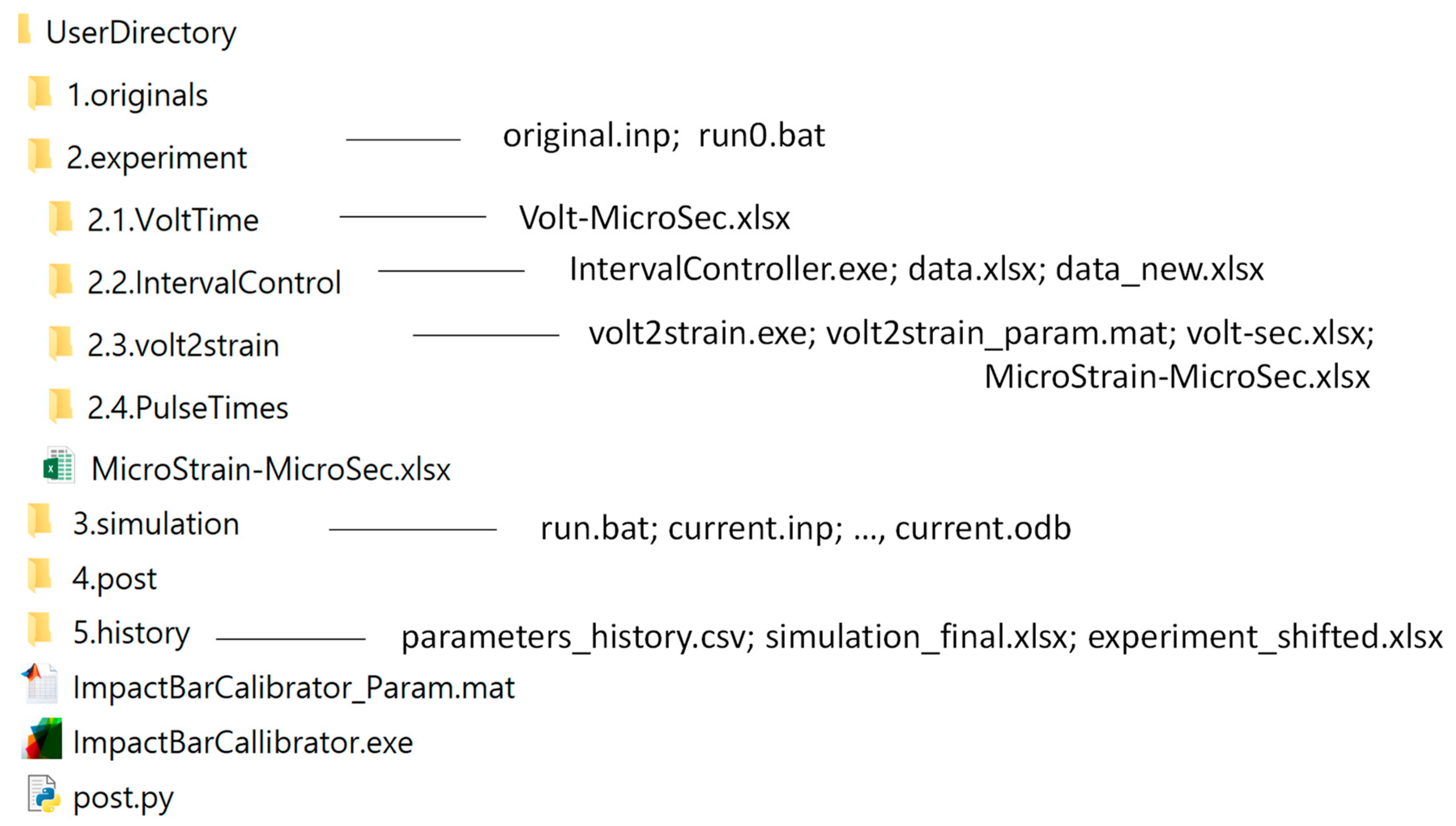
2.1. Data Structure (Directories and Files)

When the data (ImpactBarCalibrator.zip) available in [22] are downloaded and unzipped, one can observe the directories and files shown in Figure 2. The name “UserDirectory” can be changed arbitrarily (it is advised to avoid spaces and special characters in the directory name). However, the names of other directories shown in Figure 2 cannot be changed because the governing program (GP, which will be introduced later) refers to the subdirectories in Figure 2 (except for the names of the subdirectories of “2.experiment”).

Once the GP starts, it first deletes any previous files in the directories of “3.simulation” and “4.post” to empty the directories. However, it does not delete any files in “1.originals”, “2.experiment”, and “5.history”. The reason is explained later.

2.2. Roles and Relations of Files in Each Directory

This section describes the roles and relations of the files included in the presented data (Figure 2). Detailed methods for using them are explained in Section 3.

2.2.1. Root Directory

The program named “ImpactBarCalibrator.exe” in the root directory (UserDirectory) is the governing program (GP). It is a GUI program that governs the overall reverse engineering process, which exploits the ABAQUS simulations of the bar impact test. If a future revision is made, the revised GP will have new updated information in the GUI panel, and will be released in [22].

As we will explain later, the user is requested to input necessary content for the reverse engineering to the dialog box of the GP. The inputted content to the GP is stored in the “ImpactBarCalibrator_Param.mat” file.

The “post.py” file in the root directory is an execution program prepared in Python. Once the ABAQUS simulation is completed, this program extracts the simulation result from the output database file (current.odb) available in the “3.simulation” directory, and writes the “SimulatedProfile.csv” file to the “4.post” directory. The “post.py” program is executed by the GP (not directly by the user). It can be edited by right-clicking the file and selecting the “Edit with IDLE” option.

2.2.2. Directory of “1.original”

The “run0.bat” file in the “1.originals” directory is a preliminary file for preparing a batch file (run.bat) for running the ABAQUS solver. The content of the “run0.bat” file can be edited using a text editing program. It contains the following information: “call abq6131 j=current double cpus=<00> interactive”. The GP will replace the text “<00>” with the number of CPUs specified by the user. The dialog box of the GP for specifying the number of CPUs will be presented later. The GP will then write the modified command line to the “run.bat” file in the “4.simulation” directory. The text “abq6131” in the command line needs to be modified by the user depending on the version of ABAQUS and its installation environment. The “run.bat” file will launch the ABAQUS simulation using the input file named “current.inp” in the “4.simulation” directory.

The exclusive pre-post processor, ABAQUS CAE, is convenient for preparing the finite element analysis (FEA) model for the ABAQUS simulation. It assists in geometry modelling, space discretization, setting up boundary conditions, and specifying solver control options. All prepared content using the pre-post processor is saved in the *.cae and *.jnl files. The first mission of this pre-post program is to write the input file (*.inp) for the ABAQUS solver. The ABAQUS solver then carries out the FE simulation using the input file (*.inp), and writes its simulation result in the *.odb file, which is read by the ABAQUS CAE (reading the *.odb file is the second mission of this software). Because the files in the “1.original” directory are not deleted by the GP, the user can store the *.cae and *.jnl files there. It is also advantageous to store the first input file (*.inp) generated using the ABAQUS CAE in this directory.

The first-written ABAQUS input file (*.inp) must be modified and saved to the file named “original.inp” in the “1.originals” directory. How the first written ABAQUS input file needs to be modified to prepare the “original.inp” will be described later.

2.2.3. Directory of “2.experiment”

The “MicroStrain-MicroSec.csv” file is the only file referred by the GP in the “2.experiment” directory. When opened using Excel software, column A is the list of time (in micro-second unit) and column B is the strain (in micro-strain unit).

The subdirectories of the “2.experiment” directory are not referred to by the GP. They are prepared only for the user who wishes to record the pre-processing history under the “2.experiment” directory; the user can create new subdirectories here and remove any of them as well. The subdirectory named “2.1.VoltTime” is for the measured file (e.g., voltage vs. time record) using the oscilloscope. When downloaded from [22], this directory includes the voltage-time data (Volt-MicroSec.xlsx) from the as-measured version (unavailable in [22]). The necessity of the time-origin shift of the as-measured profile is described later.

Subdirectory “2.2.IntervalControl” includes “IntervalController.exe” and “data.xlsx”. The “IntervalController.exe” program reads the “data.xlsx” and outputs the “data_new.xlsx” file. The GUI panel of “IntervalController.exe” will be presented later.

Subdirectory “2.3.volt2strain” includes “volt2strain.exe”, “volt2strain_param”, and “volt-time.xlsx” files. The “volt2strain.exe” program reads the “volt-time.xlsx” file and outputs the “MicroStrain-MicroSec.xlsx” file. The parameters used in the conversion process are saved to the “volt2strain_param.mat” file. Once “volt2strain.exe” starts, it automatically reads this file and displays the read content on its dialog boxes. The GUI panel of “volt2strain.exe” will be presented later.

Subdirectory “2.4.PulseTimes” is empty when the data are downloaded/unzipped from [22]. This directory is for the user files to record the time ranges for error calculation in the reverse engineering process. The time ranges must be read from the “MicroStrain-MicroSec.xlsx” file and must be inputted to a dialog box of the GP. Therefore, the time ranges must be determined before the GP starts. Examples of the time ranges will be presented later.

2.2.4. Directory of “3.simulation”

As mentioned, the “3.simulation” directory is emptied by the GP when it runs. The GP then (i) reads the “original.inp” file from the “1.originals” directory; (ii) replaces the portions specifying the bar material properties therein (details will be explained later); and then (iii) writes the bar-property-replaced version to a file named “current.inp” in this directory. As mentioned, the GP prepares the “run.bat” file in this directory by modifying “run0.bat”, and runs the “run.bat” file to launch the ABAQUS simulation. Then, a series of simulation-induced auxiliary files (current.*) is created in this directory. When the ABAQUS simulation is completed, the “current.odb” file is written here, which is the output database of the simulation.

2.2.5. Directory of “4.post”

The GP writes the “element.txt” file in this directory by referring to its dialog box information on the history-output element. The post-processing program (post.py in the root directory) extracts strain and time information from the “current.odb” file by referring to this file (element.txt). The extracted information is written to “SimulatedProfile.csv”, which contains time vs. strain data. Column A of this file lists times in the second unit and B strain values in the non-dimensional unit.

2.2.6. Directory of “5.history”

When each simulation and post processing is completed, the GP writes (appends) the parameters employed in the simulation (E, $\nu$, and two strain correction factors) to the “parameters_history.csv” file in this directory. The error of the simulated profile (SimulatedProfile.csv) with reference to the experiment (MicroStrain-Microsec.csv) is also appended to the “parameters_history.xlsx” file. In this way, a number of rows in the “parameters_history.csv” file record the history of the parameters and error values for all reverse engineering cycles. When the reverse engineering process is completed, the GP plots the simulated profile in the final cycle (simulated_final.csv) and the experimental profile (experiment_time_shifted.xlsx).

A given reverse engineering process consists of more than dozens of simulations for the range of the foregoing parameter values. Therefore, when the reverse engineering process is completed, it is desirable to move the files in the “5.history” directory to elsewhere. The “parameters_history.csv” file should especially be moved elsewhere because it includes the results of the more than dozens of reverse engineering cycles. The user may create the “6.reults” directory, and move the file there. Even in the case where the “parameters_history.csv” file exists in this directory (5.history), the GP does not delete this file when it newly runs (to prevent accidental removal). Instead, it appends the results of the new run to existing “parameters_history.csv” file (if it does not exist, the GP creates a new file for the new run).

2.3. Required Computer Environment for Using the Data (Reverse Engineering Tools)

Before using the reverse engineering tools shown in Figure 2, the following software programs need to be installed on the user’s computer. To run compiled MATLAB [23] applications or components such as the GP here without installing MATLAB, freeware named “MATLAB Runtime” needs to be installed. Runtime 9.12 (for executable programs written in MATLAB 2022a) needs to be downloaded from [23] and installed.

Second, ABAQUS Explicit, a commercial FEA package [24], needs to be installed on the user’s computer. While there are many commercial FEA packages, the proposed GP and “post.py” program is limited to handle the ABAQUS Explicit solver. While the example ABAQUS input file available in [22] was prepared for ABAQUS Explicit version 6.13, the GP governs version-independent ABAQUS input files provided appropriate commands are used in the “run0.bat” file.

Third, freeware python (version 3.6.10 or possibly later ones) needs to be downloaded from [25] and installed. Then, as mentioned, “post.py” here can extract time and strain information from “current.odb”. Finally, commercial software Excel is needed to open “*.csv” and “*.xlsx” files.

3. Methods of Using the Data

3.1. Calibration Method of Bar Properties and Measured Strain

3.1.1. Overall Process

The method of calibrating the bar properties (E and $\nu$) and two strain correction factors consists of (i) bar density measurement and (ii) reverse engineering of the measured wave profile in a bar-alone impact test using striker. For the reverse engineering, explicit finite element simulations of the bar impact test are carried out for the range of E, $\nu$, and two strain correction factors until the simulated wave profile is reasonably consistent with the experimental counterpart. As mentioned, the parameter values employed in the reverse engineering cycle are determined as the calibrated ones when the forgoing two profiles are reasonably consistent.

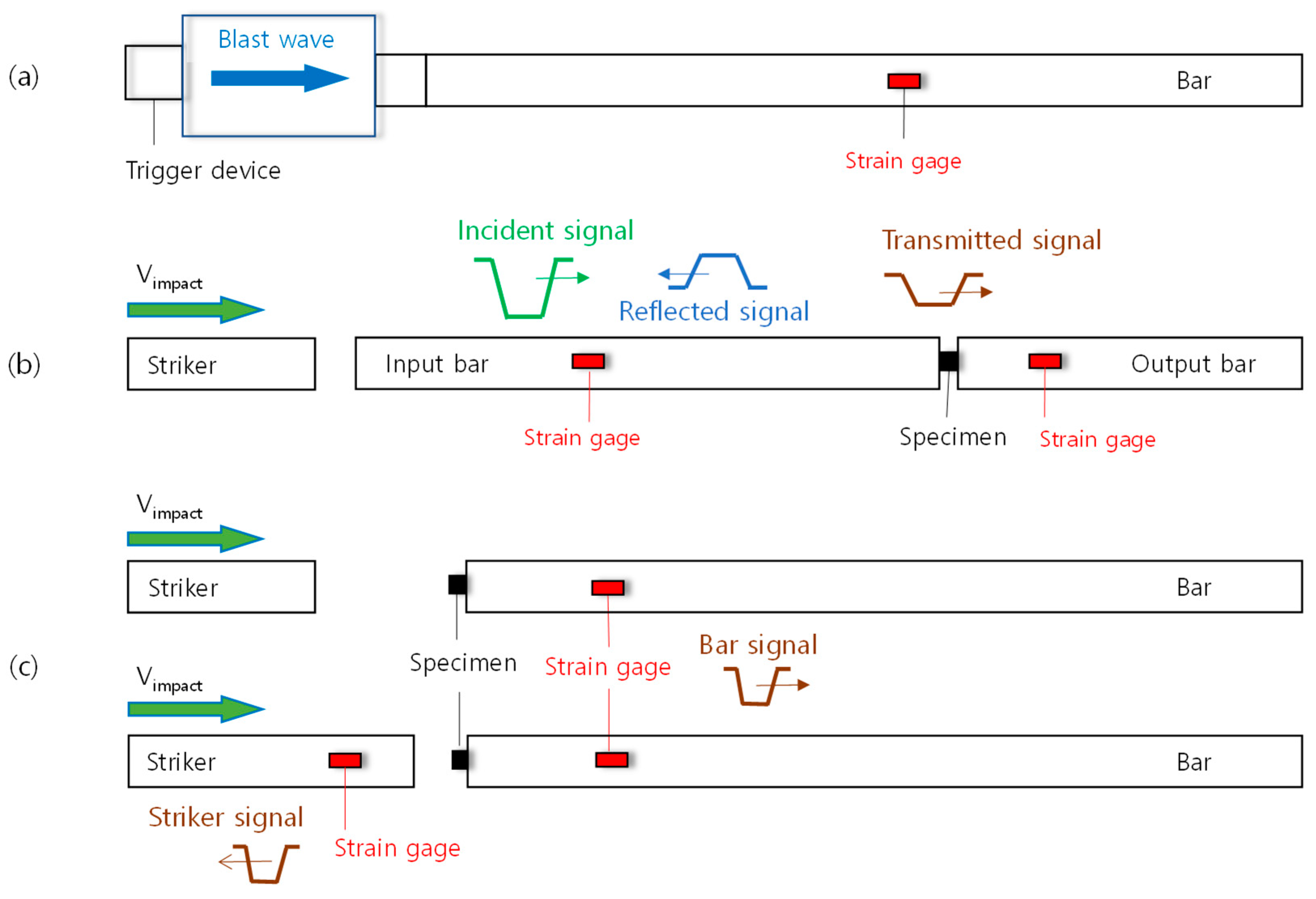
3.1.2. Bar-Alone Impact Test and Strain Measurement

The bar-alone impact test in this study indicates the split Hopkinson bar test without a specimen and without an output bar; it has only with the input bar and the striker. Both of them were introduced to our laboratory under the premise of maraging steel (C-350). The nominal diameters of the bar and striker were 19.1 mm. The impact velocity of the striker was 11.9 m/s. The bar strain was measured using equipment with a strain gage, a Wheatstone bridge (quarter bridge), and an amplifier. This measurement equipment received strain and outputted voltage to an oscilloscope, which recorded the voltage-time profile. The method for converting this profile to the strain-time profile (${\epsilon }_{\exp }\left(t\right)$) using an auxiliary program (volt2strain.exe) is described later.

3.1.3. Simulation

In the proposed reverse engineering method, the bar impact test is simulated via an explicit FEA using the ABAQUS Explicit solver. In the reverse engineering process, all simulations are carried out by employing the same density value measured separately from the impact test. However, a different set of (E, $\nu$, ${\beta }_{\mathrm{c}}$, and ${\beta }_{\mathrm{t}}$) is assumed for each reverse engineering cycle. To compare the magnitude of the simulated profile (${\epsilon }_{\mathrm{sim}}\left(t\right)$) with that of the experimental counterpart (${\epsilon }_{\exp }\left(t\right)$), the strain magnitude correction factor $\beta$ (non-dimensional) is introduced:

$$\beta {\epsilon }_{\mathrm{sim}}\left(t\right)={\epsilon }_{\exp }\left(t\right)$$

(1)

If $\beta$ is finally found to be smaller than unity ($\beta$ < 1), the experimentally determined strain profile (${\epsilon }_{\exp }\left(t\right)$) was underestimated by the strain measurement equipment, and vice versa for $\beta$ > 1. The $\beta$ value is determined separately for compression (${\beta }_{\mathrm{c}}$) and tension (${\beta }_{\mathrm{t}}$) by comparing the simulated profile with the experiment.

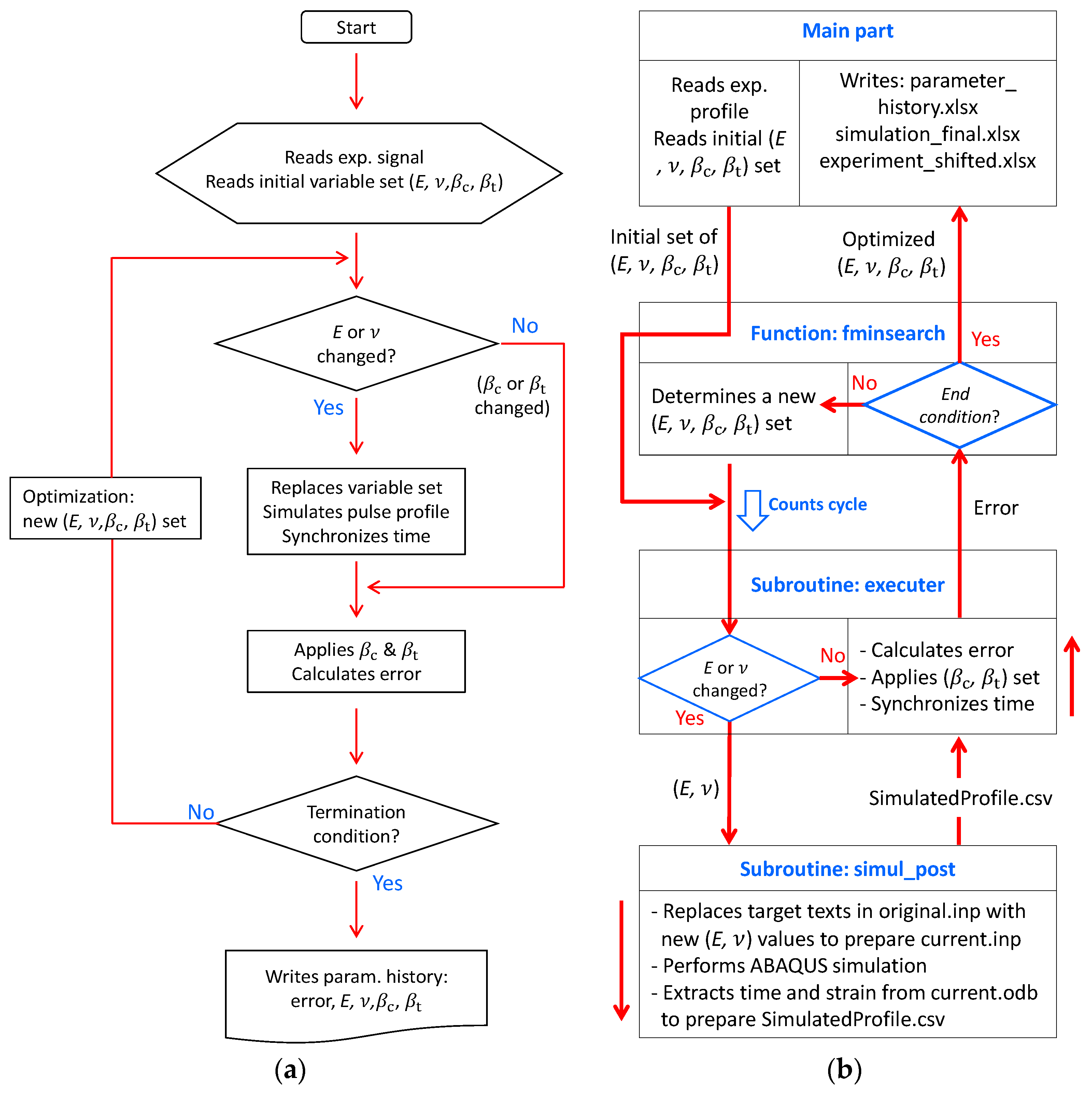
3.1.4. Reverse Engineering Algorithm

Figure 3a presents the algorithm of the reverse engineering process. In the first cycle, the GP reads the initial variable set (E, $\nu$, ${\beta }_{\mathrm{c}}$, and ${\beta }_{\mathrm{t}}$) and E and $\nu$ values substitute for the target texts in the “original.inp”. Once the first simulation is completed, the GP (i) synchronizes the times of the experimental profile with those of the simulated profile, (ii) multiplies the simulated profile by ${\beta }_{\mathrm{c}}$ and ${\beta }_{\mathrm{t}}$ values, and (iii) calculates the error between the two profiles using the formula in [20].

The reverse engineering process terminates if any of the following conditions is met [20]. First, it terminates if the predetermined (inputted) count limit by the user is reached. Second, if the inputted error limit is reached. Third, if the parameter values do not change appreciably as the number of cycles increases. This termination condition is implemented by the TolX option value in MATLAB, which was set as 10⁻⁶ in the GP.

If all of the termination conditions are unsatisfied, as can be observed in Figure 3a, a new set of (E, $\nu$, ${\beta }_{\mathrm{c}}$, and ${\beta }_{\mathrm{t}}$) is determined using the “fminsearch” function available in MATLAB for the next iteration step. If either E or $\nu$ has been changed from the values used in the previous simulation, a new explicit FEA is carried out in the next reverse engineering cycle. Otherwise, because only ${\beta }_{\mathrm{c}}$ or ${\beta }_{\mathrm{t}}$ was changed by the “fminsearch” function for the current iteration step, the explicit FEA is not carried out in the current iteration step but the simulation profile of the previous iteration step is multiplied by the new (${\beta }_{\mathrm{c}}$, ${\beta }_{\mathrm{t}}$) set. The profile obtained simply by applying a new ${\beta }_{\mathrm{c}}$ or ${\beta }_{\mathrm{t}}$ value is also called the simulated profile here although a new explicit FEA was not carried out in the current cycle; applying a new ${\beta }_{\mathrm{c}}$ or ${\beta }_{\mathrm{t}}$ value itself is regarded as a kind of simulation here. Once the new simulation profile is obtained in the current iteration cycle, the error between the simulated and experimental profiles is calculated for the current reverse engineering cycle.

As mentioned, the GP writes the history of the values for E, $\nu$, ${\beta }_{\mathrm{c}}$, and ${\beta }_{\mathrm{t}}$ used for each iteration step together with the error value of the step to the file named “parameters_history.xlsx”. If any of the termination conditions is satisfied during the reverse engineering process, as mentioned, the GP writes the strain vs. time data of the experimental profile (experiment_ shifted.xlsx) and finally the simulated one (simulation_final.xlsx). The former is the time-origin shifted version of the “MicroStrain-MicroSec.xlsx”.

Feedback among the main part and subroutines of the GP is illustrated in Figure 3b. The main part of the GP reads the initial set of (E, $\nu$, ${\beta }_{\mathrm{c}}$, and ${\beta }_{\mathrm{t}}$), which is transferred to the “fminsearch” function. In the first cycle, this function simply passes the initial values to the subroutine called “executer”, which calls another subroutine “simul_post”. This subroutine (i) replaces target texts in “original.inp” with new (E, $\nu$) values to prepare “current.inp”, (ii) performs the ABAQUS simulations, (iii) and employs “post.py”. This employed program (post.py) extracts time and strain matrices from “current.odb”, and writes ${\epsilon }_{\mathrm{sim}}\left(t\right)$ to the “SimulatedProfile.csv” file.

The executer subroutine then (i) reads “SimulatedProfile.csv”, (ii) multiplies ${\epsilon }_{\mathrm{sim}}\left(t\right)$ by the (${\beta }_{\mathrm{c}}$, ${\beta }_{\mathrm{t}}$) set, and (iii) calculates the error. If any of the termination conditions is not yet satisfied, the “fminsearch” function in MATLAB determines a new set of (E, $\nu$, ${\beta }_{\mathrm{c}}$, and ${\beta }_{\mathrm{t}}$) for the next cycle to reduce the error. As mentioned, the FEA is carried out only when the E or $\nu$ value was changed for the current cycle.

3.2. Calibration Method of Impact Velocity

If competent $V_{\mathrm{impact}}$ measurement equipment is unavailable or the strain measurement equipment is believed to be more reliable than the velocimeter, Equation (2) can be used as a way of determining the impact velocity:

$$\frac{V_{\mathrm{impact}}}{V_{\mathrm{impact}}^{\mathrm{ref}}}=\frac{{\epsilon }_{\exp }\left(t\right)}{{\epsilon }_{\mathrm{sim}}^{\mathrm{ref}}\left(t\right)}$$

(2)

In Equation (2), $V_{\mathrm{impact}}^{\mathrm{ref}}$ is an arbitrarily set impact velocity (e.g., 10 m/s) where ${\epsilon }_{\mathrm{sim}}^{\mathrm{ref}}\left(t\right)$ is obtained. To use Equation (2), the bar properties need to be pre-calibrated to obtain the simulated profile (${\epsilon }_{\mathrm{sim}}^{\mathrm{ref}}\left(t\right)$) at the reference impact velocity. The 1D method [20,21] that does not need $V_{\mathrm{impact}}$ information is suitable for such pre-calibration of bar properties. The GP renders the ABAQUS simulation at the user-specified reference velocity to obtain ${\epsilon }_{\mathrm{sim}}^{\mathrm{ref}}\left(t\right)$, followed by determining the $V_{\mathrm{impact}}$ value with reference to a reliably measured ${\epsilon }_{\exp }\left(t\right)$ using Equation (2).

3.3. Pre-Processing for Using Governing Program

3.3.1. Preparing Voltage vs. Time Profile (in Directory “2.1.VoltTime”)

The voltage vs. time data are experimentally measured using an oscilloscope. We prepared the data file in Excel format: “Volt-MicroSec.xlsx” in the “2.VoltTime” directory. The time data (in $\mathsf{\mu }$s unit) are in column A and the voltage data (in volt unit) are in B. The sign of this file should be positive in tension.

The time origin of the measured voltage-time data is usually arbitrary. It is advisable to shift the time origin of the raw data in such a way that the time of the first hill of the incident pulse is less than or equal to that in the simulated profile. Then, one can avoid an unnecessarily long pre-incident pulse portion in the experimental profile. An example of the voltage-time data in this way is in “Volt-MicroSec.xlsx” file.

Then, the GP synchronizes the time of the first hill to that of the simulated profile after each simulation. The end time of the experimental profile (Volt-MicroSec.xlsx) does not need to be exactly the same as that of the simulated profile but both of them are recommended to be close.

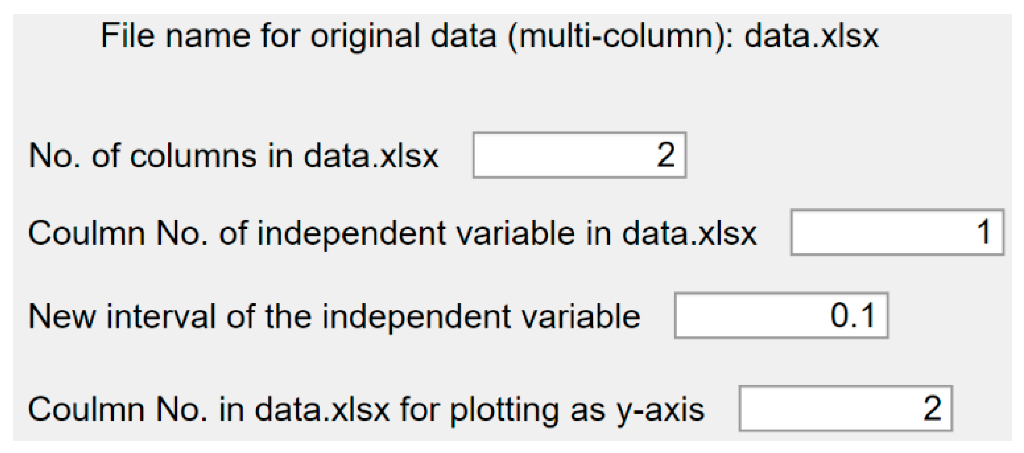
3.3.2. Interval Control of Voltage vs. Time Profile (in Directory “2.2.IntervalControl”)

Most of the recorded data (voltage vs. time) in the experiment were at 0.1 $\mathsf{\mu }$s intervals while some intervals were approximately 0. 1 $\mathsf{\mu }$s. To use the recorded data for dispersion-correction purposes [20,21], the time intervals need to be made constant (e.g., 0.1 $\mathsf{\mu }$s). The GP for the 3D method also requests constant time intervals in “Volt-MicroSec.xlsx”. To make the time intervals constant, the “IntervalController.exe” program available in [22] can be used.

The dialog box of the “IntervalController.exe” program is shown in Figure 4. This program reads the “data.xlsx” file, requests the user to input a new interval value, and outputs “data_new.xlsx”. The “Volt-MicroSec.xlsx” file should be copied to this directory and renamed to “data.xlsx”. The “IntervalController.exe” program can handle multicolumn data.

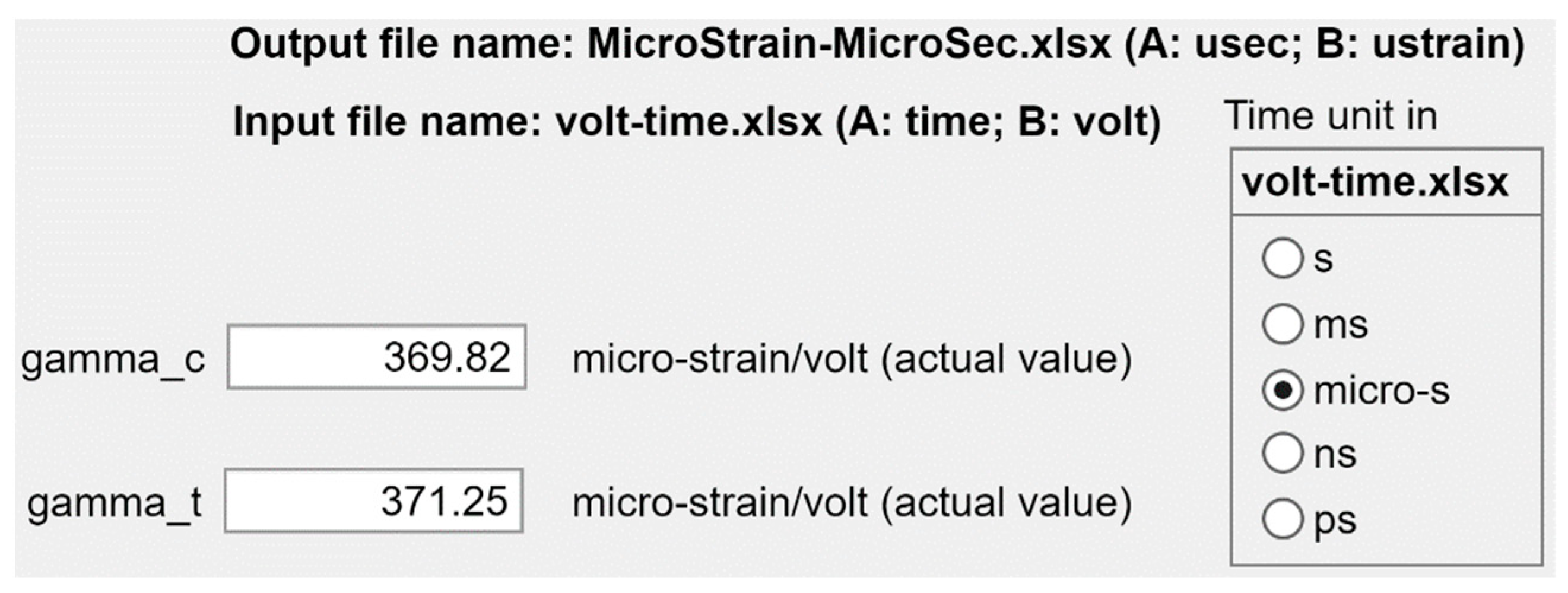
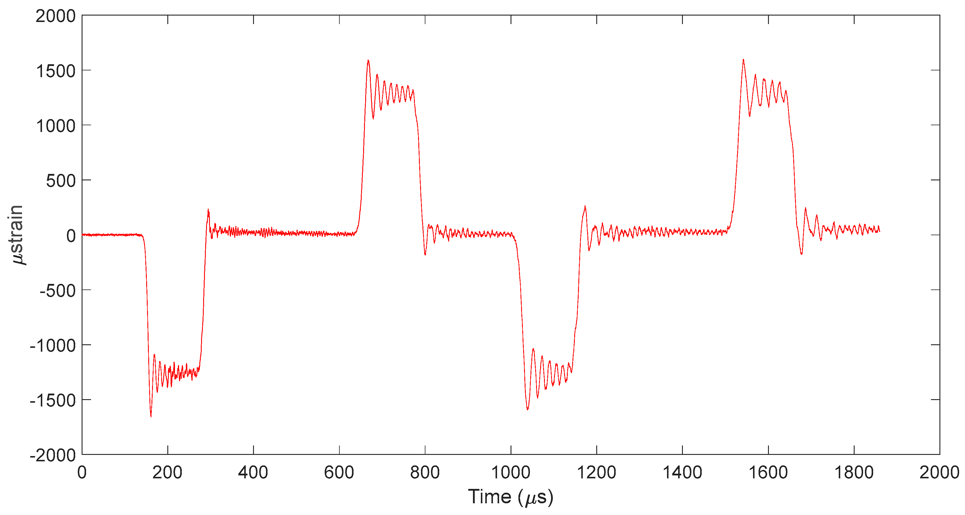
3.3.3. Preparing Strain vs. Time Profile (in Directory “2.3.volt2strain”)

The strain vs. time profile can be obtained from the voltage-time profile using information on the strain-per-volt ratio ($\gamma$) of the measurement equipment:

$${\epsilon }_{\exp }\left(t\right)=\gamma V\left(t\right)$$

(3)

The employed measurement equipment exhibited slightly different $\gamma$ values in compression (${\gamma }_{\mathrm{c}}$) and tension (${\gamma }_{\mathrm{t}}$). Their values were 369.82 and 371.25 $\mathsf{\mu }\mathrm{st}/V$, respectively, just before the impact test was carried out. To apply these values to the voltage-time profile obtained in the bar impact test, a GUI program, “volt2strain.exe [22], can be used.

The dialog box of the “volt2strain.exe” program is shown in Figure 5. When this program starts, it reads its auxiliary file (volt2strain_pram.mat), and displays the read content in the dialog box. The user can modify the content in the dialog box, and save it to the auxiliary file. In this way, the “volt2strain_pram.mat” file records how the voltage vs. time data was converted to the strain vs. time data.

Once the run button is clicked, the “volt2strain.exe” program reads the “volt-time.xlsx” file. This input file can be prepared by copying the “data_new.xlsx” to this directory and renaming it to “volt-time.xlsx”. Column A of this file is supposed to be time data (in ms, $\mathsf{\mu }$s, ns, or ps) and B voltage (in volt unit). The “volt2strain.exe” program applies the ${\gamma }_{\mathrm{c}}$ and ${\gamma }_{\mathrm{t}}$ values to the volt vs. time data and outputs “MicroStrain-MicroSec.xlsx” file; the units in the written file are μstrain and $\mathsf{\mu }$s. It is necessary to copy (or move) this file to the “2.Experiment” directory. As mentioned, only the “MicroStrain-MicroSec.xlsx” file in the “2.experiment” will be read later by the GP. The strain vs. time profile prepared in this way is presented in Figure 6.

After the “MicroStrain-MicroSec.xlsx” file is prepared, it is necessary to identify the time ranges to be used for error calculation in the reverse engineering process. One can use commercial software such as Origin Lab to identify the time points in the experimental profile. We recommend saving the file used for the time point identification in the “2.4.PulseTimes” directory for later reference. Reference [22] does not provide the file used for the time point identification. However, the identified time values of the measured profile in Figure 6 will be presented later (in dialogue box of the GP; “Time Ranges of Pulses” tab).

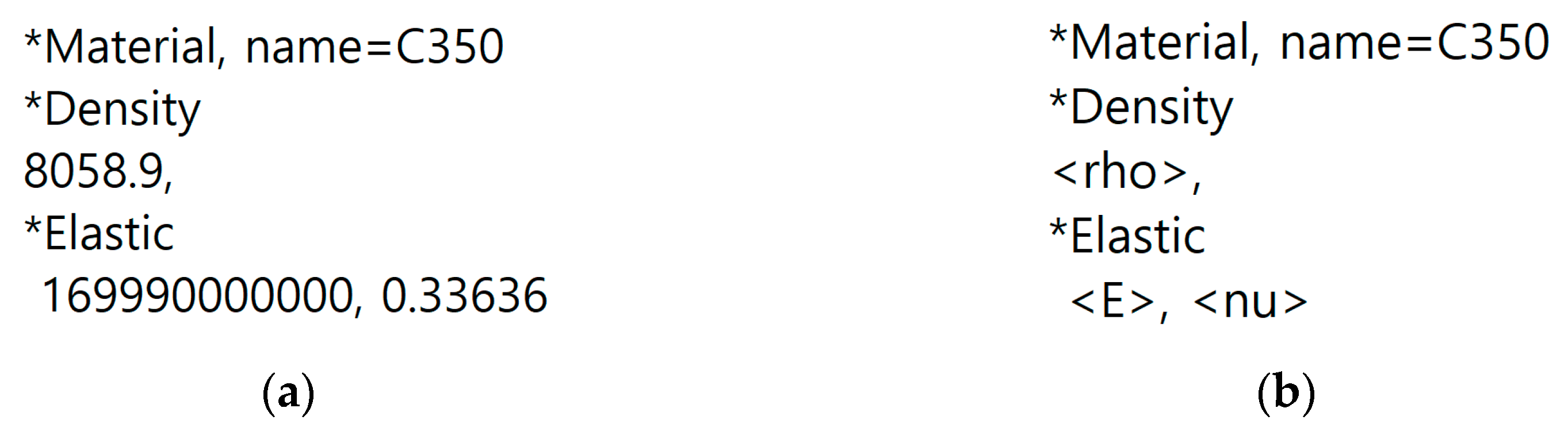
3.3.4. Preparing “original.inp”

The next pre-processing for using the GP is the preliminary ABAQUS simulation of the bar impact test. All ABAQUS simulations need to be carried out in the m-kg-s unit because the GP assumes this unit system in the ODB file. Two elastic constants (e.g., E and $\nu$) and $\rho$ are necessary for an explicit FEA. In our separate study, it was necessary to separately measure $\rho$ and determine $\nu$ and $c_{\mathrm{o}}$ via the iterative dispersion correction process [20,21]. Then, E is determined via the equation: $E=\rho c_{\mathrm{o}}^2$. The bar properties obtained in this way were: $\rho$ = 8058.9 kg/m³, E = 169.99 GPa, $\nu$ = 0.336355 ($c_{\mathrm{o}}$ = 4592.755045 m/s), which were inputted as the initial bar material properties in the first FEA.

Once the preliminary simulation is completed, the ABAQUS input file (*.inp) used for the preliminary simulation has to be modified. Figure 7 presents an example of the modification, which shows the portion of the input file before and after the modification. It is observed that the values of material properties (E, $\rho$, and $\nu$) were modified to “<E>”, “<rho>”, and “<nu>”, respectively, which are called the target texts here. These target texts were employed simply because the foregoing texts do not appear in a standard ABAQUS input file (*.inp). The user can employ other target texts provided they do not appear in the standard input file. The modified input file has to be saved to the file named “original.inp” as this file name is referred to by the GP.

As we will show later, the user is supposed to input the target texts to the dialog box of the GP to let it replace the target texts in the “original.inp” file with the assumed values in each simulation. The GP subsequently writes the replaced input file version to “current.inp”, which is to be used for the ABAQUS simulation in the reverse engineering process.

3.4. Tips for Using Governing Program

3.4.1. Load, Save, and Run

When the GP (BarImpactCalibrator.exe) starts, it automatically loads information from the “ImpactBarCalibrator_Param.mat” file to its dialog box. The user can edit and save them. The saved content can be loaded via the load button in the GUI panel.

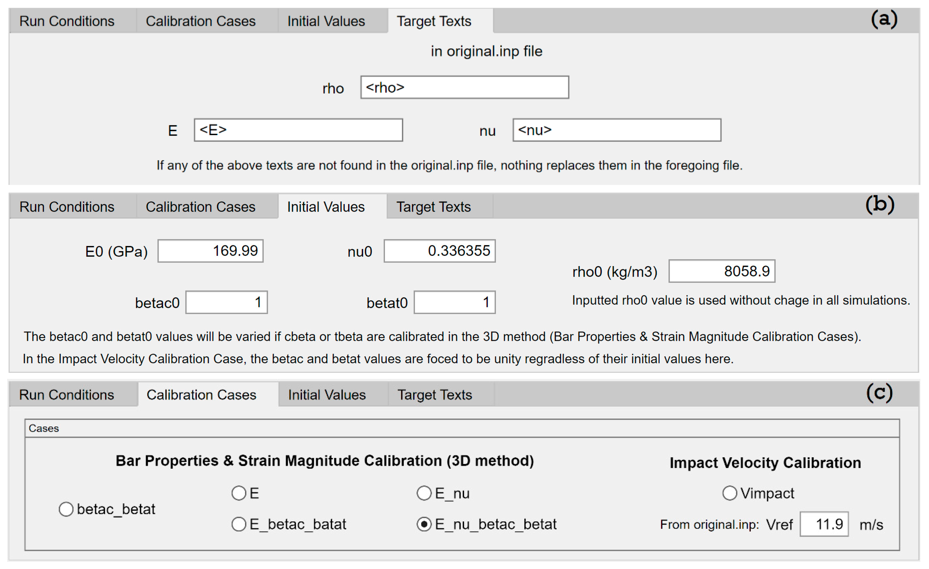
3.4.2. “Target Texts” Tab

Figure 8a shows the “Target Text” tab of the GP. The GP searches these inputted target texts in the “original.inp” file. Therefore, the target texts in the dialog box and those in the “original.inp” file should match. If the inputted target texts in the tab (edit field) are found in the “original.inp” file, the GP replaces them with the corresponding values in the “Initial Values” tab. As mentioned, the replaced version will be written to the “current.inp” file.

If any of the inputted target texts in this tab are not in the “original.inp” file, the GP ignores the replacement of such target texts. Then, the “current.inp” file will include some un-replaced target texts (e.g., <E>, <nu>, <rho>), which cannot be recognized by the ABAQUS solver. Then, an error occurs in the first simulation of the reverse engineering process.

3.4.3. “Initial Values” Tab

The “Initial Values” tab of the GP is shown in Figure 8b. As mentioned, the values of E, $\nu$, and $\rho$ inputted to this tab will substitute for the corresponding target texts (<E>, <nu>, <rho>, respectively) in the “original.inp” file. Because the density value was separately measured from the bar impact test, it is unchanged during the later simulations of the bar impact test. Nevertheless, the dialog box requests the user to input the density value to make sure the inputted density value into the simulation. In all simulations, the GP replaces the target text for $\rho$ (<rho>) with the initially inputted value in this tab.

The initial values of ${\beta }_{\mathrm{c}}$ (betac0) and ${\beta }_{\mathrm{t}}$ (betat0) inputted by the user are not used for the replacement of any texts in the “original.inp” file because these values are not used for the ABAQUS simulation. They are used once the FEA using ABAQUS is completed; the simulated wave profile is multiplied by them. The “betac0” and “betat0” values will vary only when the ${\beta }_{\mathrm{c}}$ or ${\beta }_{\mathrm{t}}$ value is calibrated by selecting the calibration case of “betac_betat” in the “Calibration Cases” tab. In all other calibration cases, the inputted values (betac0 and betat0) are used without change.

3.4.4. “Calibration Cases” Tab

Figure 8c shows the “Calibration Cases” tab of the GP. Section 3.1 described the case where four variables (E, $\nu$, ${\beta }_{\mathrm{c}}$, and ${\beta }_{\mathrm{t}}$) were calibrated via the reverse engineering of the wave profile. For the case of the experimental wave profile here (Figure 6), the four variables could be calibrated directly via the calibration case of “E_nu_betac_betat”.

Nevertheless, the GP copes with the cases where the user wants to calibrate the variables step by step for their own experimental wave profiles. One may want to calibrate only the (${\beta }_{\mathrm{c}}$, ${\beta }_{\mathrm{t}}$) set first via the calibration case of “betac_betat” (see Figure 8c). In such a case, the calibrated values of ${\beta }_{\mathrm{c}}$ and ${\beta }_{\mathrm{t}}$ may be slightly different from the finally calibrated ones via the calibration case of “E_nu_betac_betat” because the calibration of only the (${\beta }_{\mathrm{c}}$, ${\beta }_{\mathrm{t}}$) set is generally carried out when the bar properties are not yet calibrated. In other words, in the calibration case of “betac_betat”, the (${\beta }_{\mathrm{c}}$, ${\beta }_{\mathrm{t}}$) set is performed under the condition that the simulated hills and valleys in the plateau of the pulse are not fully coincident with the experiment. They will be consistent with the experimental counterpart only when all of the four variables are calibrated.

In the calibration case of the “betac_betat”, the first simulation is carried out using the initial values of the four variables (E0, nu0, betac0, and betat0). Because E and $\nu$ values are the same in the subsequent simulations in this case (see the flow chart in Figure 3), no further finite element analyses are carried out from the second cycle. From the second cycle, only the ${\beta }_{\mathrm{c}}$ or ${\beta }_{\mathrm{t}}$ value is varied and applied to the simulated profile of the first cycle. Therefore, the speed of calibrating the (${\beta }_{\mathrm{c}}$, ${\beta }_{\mathrm{t}}$) set is very fast as compared with other calibration cases where a number of finite element analyses are required. In this regard, it is advised to carry out the calibration case of “betac_betat” first by using reasonably guessed initial values of the four variables. This should assist in other subsequent calibration cases listed in the tab. The calibration case of the “E_nu_betac_betat” should be carried out finally, which yields the finally calibrated values of the four variables. However, as mentioned, the experimentally measured profiles in the author’s laboratory could be successfully calibrated directly via the calibration case of “E_nu_betac_betat”.

In the 3D method, the ${\beta }_{\mathrm{c}}$ and ${\beta }_{\mathrm{t}}$ values are calibrated with reference to a given impact velocity (11.9 m/s here). Under the assumption that the strain was measured more reliably than the impact velocity, the $V_{\mathrm{impact}}$ value can be determined with reference to ${\epsilon }_{\exp }\left(t\right)$ by selecting the “Vimpact” calibration case in the current tab. The GP then renders the simulation of the bar impact test once at a reference impact velocity ($V_{\mathrm{impact}}^{\mathrm{ref}}$), and calculates the $V_{\mathrm{impact}}$ value using Equation (2). In such a case, the bar properties inputted to the “Initial Values” tab are used. As for the values of “betac” and “betat”, they are forced to be unity regardless of their values inputted in the “Initial Values” tab.

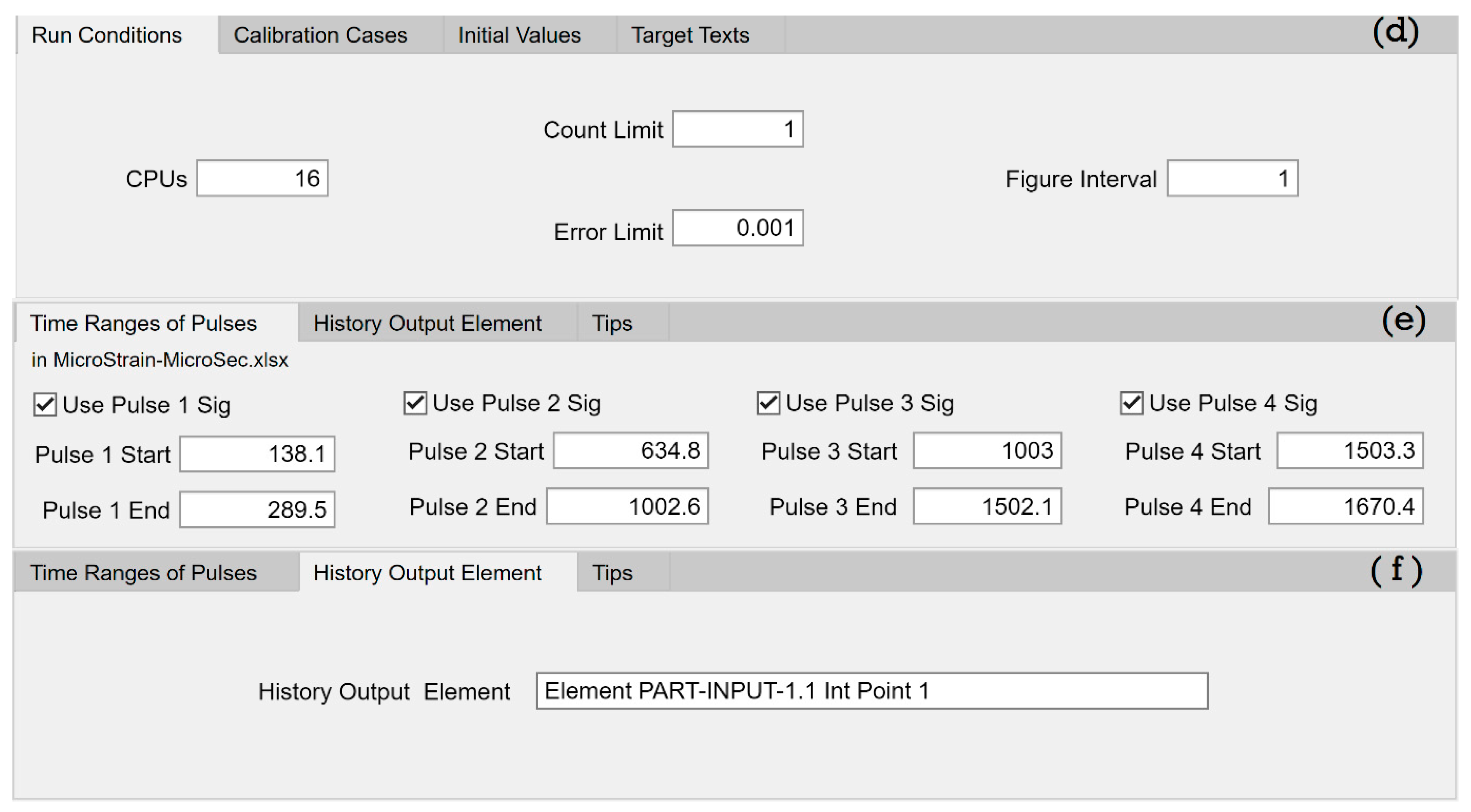
3.4.5. “Run Conditions” Tab

The “Run Conditions” tab of the GP is presented in Figure 8d. The edit field “CPUs” is for the number of computer threads to be used for the ABAQUS simulation. As mentioned, the GP substitutes the inputted value in the “CPUs” edit field for the target text “<cpus>” in the “run0.bat” file, and writes the substituted version to the “run.bat” file. This file includes a list of disk operating system (dos) commands for running the ABAQUS Explicit solver.

The inputted value in the “Count Limit” edit field is the maximum number of cycles in the reverse engineering process. The count limit is one of the termination conditions of the process, at which the figure comparing the experimental profile with the reverse-engineered counterpart in the final cycle is plotted. If the user sets the “Count Limit” value as unity at a given initial value set of (E, $\nu$, ${\beta }_{\mathrm{c}}$, and ${\beta }_{\mathrm{t}}$), the simulated profile at the inputted set is plotted in comparison with the experimental profile. For such a purpose, any “Simulation Case” can be selected. This technique of setting the “Count Limit” value as unity is useful in investigating the influence of the individual variable (or a given variable set) on the simulated profile with reference to the experimental counterpart.

The inputted value to “Error Limit” edit field is the error level below which the reverse engineering loop terminates. This value can be set to a sufficiently small number such as 0.001 together with a sufficiently large count limit value. Then, the loop terminates by the third termination condition, the TolX option of MATLAB [23]. This way of controlling the termination condition is recommended for the usual calibration process.

When each cycle of the reverse engineering process is completed, the GP can plot the figure that compares the simulated profile with its experimental counterpart. The inputted value to the “Figure Interval” edit field controls how often the figure is plotted. The figure interval value of n means that the figure is plotted at every nth cycle of the reverse engineering process.

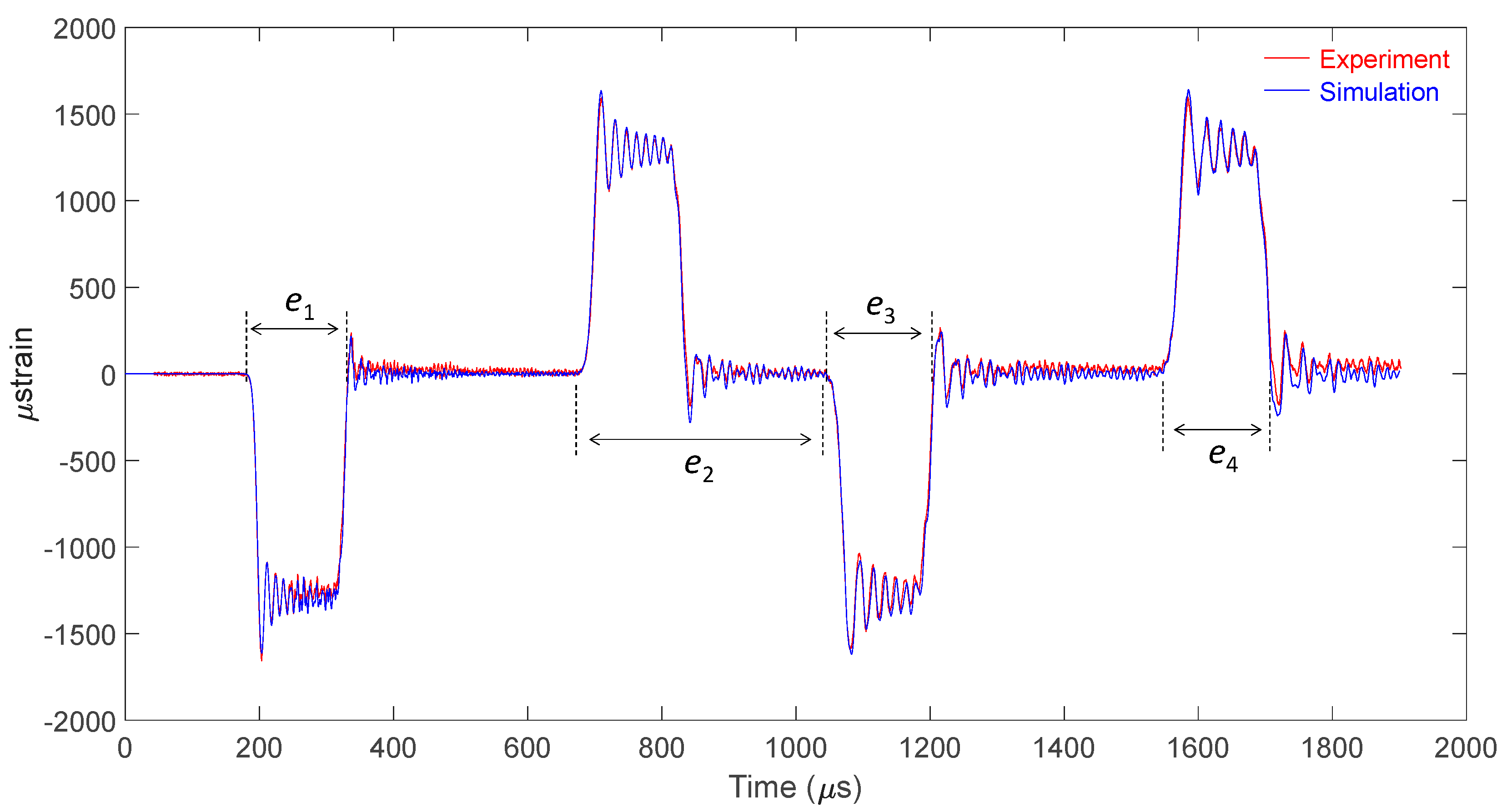
3.4.6. “Time Ranges of Pulses” Tab

Figure 8e presents the “Time Ranges of Pulses” tab of the GP. The proposed method of calibration utilizes up to four pulses in the bar-alone impact test. The inputted time ranges in this tab are used for the error calculation.

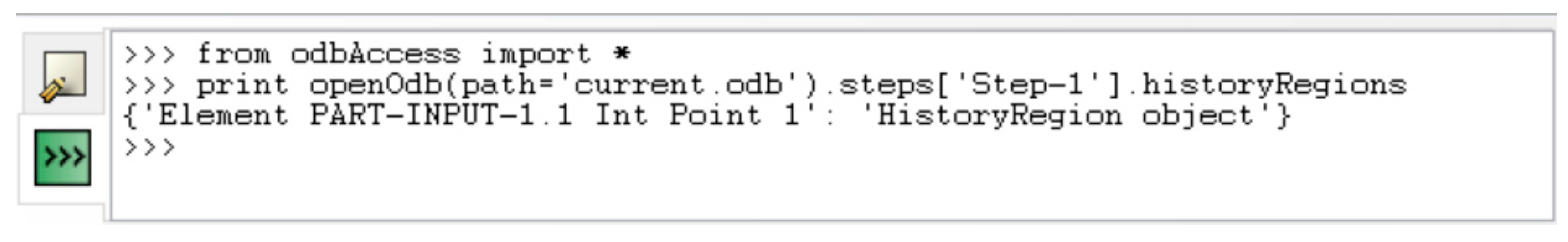
3.4.7. “History Output Element” Tab

The “History Output Element” tab of the GP is presented in Figure 8f. The GP transfers specified element information in this tab to its sub-governing program (post.py), which extracts the strain of the specified element from the “current.odb” file. As mentioned, this sub-program (post.py) writes the extracted content to the “SimulatedProfile.csv” file.

To obtain the text information to be inputted to the “History Output Element” edit field (Element PART-INPUT-1.1 Int Point 1), one can open the “current.odb” file using ABAQUS CAE, select the “File” menu, and go to “ABAQUS PDE”. Then, the ABAQUS PDE dialog box will pop up (see Figure 9). Click “<<<” icon, and copy/paste the following two lines at a time:

$$\begin{array}{l}\mathrm{from}\mathrm{odbAccess}import*\\ \mathrm{print}\mathrm{openOdb}(\mathrm{path}=‘\mathrm{current}.\mathrm{odb}’).\mathrm{steps}[‘\mathrm{Step}\text{-}1’].\mathrm{historyRegions}\end{array}$$

where “Step-1” is the step name in the ABAQUS input file (named in the ABAQUS CAE). Then, the following line will be displayed in the dialog box: “{’Element PART-INPUT-1.1 Int Point 1’: ’HistoryRegion object’}”, which includes the text shown in the edit field of Figure 8f.

3.5. Calibration Result and Discussion

3.5.1. Bar Properties and Measured Strain (3D Method)

When the reverse engineering process is completed for the calibration cases of the bar properties and measured strain, the GP plots the reverse-engineered result in the final cycle together with the experimental profile. Figure 10 presents an example, and the figure includes the error calculation ranges (e₁–e₄) which were selected arbitrarily. The error in the specified time ranges were calculated using the formula in [20] and weight-averaged considering the number of data points in the respective time ranges. The weight-averaged error was minimized in the reverse engineering process.

According to the “history_parameters.xlsx” file, the calibrated values for the experimental profile shown in Figure 6 were E = 170.008486 GPa, $\nu$ = 0.333145, ${\beta }_{\mathrm{c}}$= 0.978866, and ${\beta }_{\mathrm{t}}$ = 0.995751 (separately measured $\rho$ value was 8058.9 kg/m³). The $c_{\mathrm{o}}$ (= $\sqrt{E/\rho }$) value was determined to be 4593.0 m/s. These determined values of E, $\nu$, and $c_{\mathrm{o}}$ are different from the separately determined values via the 1D method [20,21] by only 0.01, 0.96, and 0.01%, respectively.

The calibrated values of ${\beta }_{\mathrm{c}}$ and ${\beta }_{\mathrm{t}}$ were 0.978866 and 0.995751, respectively: they were slightly lower than unity. This observation indicates that the strain magnitudes (in compression and tension, respectively) were slightly underestimated in the experiment with reference to the measured impact velocity (11.9 m/s).

3.5.2. Impact Velocity

In the 3D method, ${\beta }_{\mathrm{c}}$ and ${\beta }_{\mathrm{t}}$ values were calibrated with reference to a given impact velocity. If we assume that the strain was measured without error, the $V_{\mathrm{impact}}$ value was slightly overestimated. Under such an assumption, the $V_{\mathrm{impact}}$ value was calibrated using the GP (calibration case of “Vimpact”); the result for the profile in Figure 6 was 11.7307 m/s; the measured value (11.9 m/s) using a velocimeter was overestimated by approximately 1.44% with reference to the measured strain.

3.5.3. Further Discussion

In this study, we successfully used the proposed program in our laboratory for steel and aluminium-based bars at a range of impact velocities. Although the algorithm presented here can also be used for polymer-based viscoelastic bars, the current version of the program is limited to metallic bars simply because the dialog box of the program does not receive visco-elastic parameters of the bar (such as Prony series).

There should not be a temperature gradient in the bar during the bar-alone impact test for calibration purposes because the pulse length and arrival time of the pulse is altered due to the temperature gradient. To use the current program for calibrating the properties (E and $\nu$) of the bar used in a high-temperature spilt Hopkinson bar where the temperature gradient of the bar usually exists, the temperature-dependency of bar properties (E, $\nu$ and $\rho$) should be known for simulation.

4. User Notes

User feedback of the program is welcomed. Any updated programs in the future will be released in [22].

References

1. Hopkinson, B. A Method of measuring the pressure produced in the detonation of high explosives or by the impact of bullets. Philos. Trans. R. Soc. Lond. Ser. A 1914, 213, 437–456. [Google Scholar] [CrossRef]
2. Davies, R.M. A critical study of the Hopkinson pressure bar. Philos. Trans. R. Soc. A 1948, 240, 375–457. [Google Scholar]
3. Kolsky, H. An investigation of the mechanical properties of materials at very high rates of loading. Proc. Phys. Soc. Lond. Sect. B 1949, 62, 676–700. [Google Scholar] [CrossRef]
4. Chen, W.; Song, B. Split Hopkinson (Kolsky) Bar—Design, Testing, and Applications; Springer Science+Business Media, LLC: New York, NY, USA, 2011. [Google Scholar]
5. Othman, R. The Kolsky–Hopkinson Bar Machine; Springer International Publishing: Cham, Switzerland, 2018. [Google Scholar]
6. Shin, H.; Kim, J.-B. Evolution of specimen strain rate in split Hopkinson bar test. Proc. Inst. Mech. Eng. Part C J. Mech. Eng. Sci. 2019, 233, 4667–4687. [Google Scholar] [CrossRef] [Green Version]
7. Shin, H.; Kim, D. One-dimensional analyses of striker impact on bar with different general impedance. Proc. Inst. Mech. Eng. Part C J. Mech. Eng. Sci. 2020, 234, 589–608. [Google Scholar] [CrossRef]
8. Shin, H.; Kim, S.; Kim, J.-B. Stress transfer mechanism of flange in split Hopkinson tension bar. Appl. Sci. 2020, 10, 7601. [Google Scholar] [CrossRef]
9. Shin, H.; Lee, J.-H.; Kim, J.-B.; Sohn, S.-I. Design guidelines for the striker and transfer flange of a split Hopkinson tension bar and the origin of spurious waves. Proc. Inst. Mech. Eng. Part C J. Mech. Eng. Sci. 2020, 234, 137–151. [Google Scholar] [CrossRef]
10. Shin, H.; Kim, J.-B. Understanding the anomalously long duration time of the transmitted pulse from a soft specimen in a Kolsky bar experiment. Int. J. Precis. Eng. Manufact. 2016, 17, 203–208. [Google Scholar] [CrossRef]
11. Dharan, C.K.H.; Hauser, F.E. Determination of stress-strain characteristics at very high strain rates. Exp. Mech. 1970, 10, 370–376. [Google Scholar] [CrossRef]
12. Couque, H. The use of the direct impact Hopkinson pressure bar technique to describe thermally activated and viscous regimes of metallic materials. Phil. Trans. R. Soc. A 2014, 372, 20130218. [Google Scholar] [CrossRef] [PubMed] [Green Version]
13. Govender, R.A.; Curry, R.J. The ‘‘open’’ Hopkinson pressure bar: Towards addressing force equilibrium in specimens with non-uniform deformation. J. Dyn. Behav. Mater. 2016, 2, 43–49. [Google Scholar] [CrossRef] [Green Version]
14. Shin, H.; Ju, Y.; Choi, M.-K.; Ha, D.H. Flow stress description characteristics of some constitutive models at wide strain rates and temperatures. Technologies 2022, 10, 52. [Google Scholar] [CrossRef]
15. Shin, H.; Kim, J.-B. A Phenomenological constitutive equation to describe various flow stress behaviors of materials in wide strain rate and temperature regimes. J. Eng. Mater. Technol. 2010, 132, 021009. [Google Scholar] [CrossRef]
16. Lee, W.; Lee, H.-J.; Shin, H. Ricochet of a tungsten heavy alloy long-rod projectile from deformable steel plates. J. Phys. D Appl. Phys. 2002, 35, 2676–2686. [Google Scholar] [CrossRef] [Green Version]
17. Shin, H.; Lee, H.-J.; Yoo, Y.-H.; Lee, W. A determination procedure for element elimination criterion in finite element analysis of high-strain-rate impact/penetration phenomena. JSME Int. J. 2004, 47, 35–41. [Google Scholar] [CrossRef] [Green Version]
18. Soares, G.C.; Hokka, M. Synchronized full-field strain and temperature measurements of commercially pure titanium under tension at elevated temperatures and high strain rates. Metals 2022, 12, 25. [Google Scholar] [CrossRef]
19. Shin, H. Pochhammer–Chree equation solver for dispersion correction of elastic waves in a (split) Hopkinson bar. Proc. Inst. Mech. Eng. Part C J. Mech. Eng. Sci. 2022, 236, 80–87. [Google Scholar] [CrossRef]
20. Shin, H. Sound speed and Poisson’s ratio calibration of (split) Hopkinson bar via iterative dispersion correction of elastic wave. J. Appl. Mech. 2022, 89, 061007. [Google Scholar] [CrossRef]
21. Shin, H. Manual for calibrating sound speed and Poisson’s ratio of (split) Hopkinson bar via dispersion correction using Excel and Matlab templates. Data 2022, 7, 55. [Google Scholar] [CrossRef]
22. Shin, H. GUI Program Governing ABAQUS Simulations of Bar Impact Test for Calibrating Bar Properties, Measured Strain, and Impact Velocity (Version 20230218). Zenodo. Available online: https://doi.org/10.5281/zenodo.7652652 (accessed on 24 February 2023).
23. MathWorks®. MATLAB Runtime. Available online: https://kr.mathworks.com/products/compiler/matlab-runtime.html (accessed on 18 February 2023).
24. Simuleon, Technia Company. SIMULIA Abaqus, Non-Linear Finite Element Analysis. Available online: https://www.simuleon.com/simulia-abaqus/ (accessed on 24 February 2023).
25. pythonTM. Version 3.10.6. Available online: https://www.python.org/downloads/ (accessed on 24 February 2023).
Figure 1. Schematic of the (a) Hopkinson bar, (b) split Hopkinson bar, and (c) direct impact Hopkinson bar. In (c), the specimen can also be positioned at the striker side.
Data 08 00054 g001
Figure 2. Structure of the data (reverse engineering tools).
Data 08 00054 g002
Figure 3. (a) Algorithm of the reverse engineering process. (b) Feedbacks among the main part and subroutines of the GP.
Data 08 00054 g003
Figure 4. Dialog box of the “IntervalController.exe” program.
Data 08 00054 g004
Figure 5. Dialog box of the “volt2strain.exe” program.
Data 08 00054 g005
Figure 6. Experimental profile of strain (data in MicroStrain-MicroSec.xlsx).
Data 08 00054 g006
Figure 7. Examples of the ABAQUS input file portion, which specifies the bar material properties in m-kg-sec unit. (a) Before and (b) after modification.
Data 08 00054 g007
Figure 8. The tabs in the dialog box of the GP: (a) “Target Texts”, (b) “Initial Values”, (c) “Calibration Cases”, (d) “Run Conditions”, (e) “Time Ranges of Pulses”, and (f) “History Output Element”.
Data 08 00054 g008aData 08 00054 g008b
Figure 9. ABAQUS PDE dialog box and commands for displaying history output element information.
Data 08 00054 g009
Figure 10. Result of the reverse engineering process using the GP in comparison with the experimental profile.
Data 08 00054 g010
Disclaimer/Publisher’s Note: The statements, opinions and data contained in all publications are solely those of the individual author(s) and contributor(s) and not of MDPI and/or the editor(s). MDPI and/or the editor(s) disclaim responsibility for any injury to people or property resulting from any ideas, methods, instructions or products referred to in the content.