We now describe how we obtained, processed, and analyzed the data.
Section 3.1 explains the operational rather than clinical nature of the data, and it explains the usage approval obtained.
Section 3.2 describes the collection and preprocessing of the raw data.
Section 3.3 details the process of computing the derived service time.
Section 3.4 introduces how to handle outliers.
Section 3.5 presents the exploratory data analysis of the prepared data and insights about the results.
3.2. Create the Raw Data Files
Authorized clinic personnel directly extracted the clinic’s stellar physician’s 2018 and 2019 consultation records from the clinic’s information system. Then, the following steps were taken to protect patients’ private information:
The records were reviewed by the clinic and marked whether the consultation was related to cancer (the
M.Cancer and
S.Cancer in
Table 2), and then the original diagnosis information was removed.
Each patient was assigned a unique ID by Hangu, which was then encrypted during the creation of the raw dataset. We ensured that each patient’s encrypted ID is unique, yet patients’ true identities are deidentified after such encryption.
The date of each session was removed. Potentially useful information related to the date was preserved in the following way:
- –
The date information was turned into the variables Month and DayOfWeek.
- –
We added a variable indicating whether a session occurred during a working day or a holiday. The dates of public holidays in China depend on the lunar calendar and the solar one; thus, the national holiday arrangement changes yearly. When tagging each session, we checked the 2018 and 2019 official public holiday arrangements [
30,
31].
- –
Each session was given a unique ID between 1 and 381, which preserved the actual chronological order. Future data users can recreate all the sessions of the focal physician and the order and length of each patient’s consultation.
Raw_1.csv was created following the above steps. In total, 6853 consultation-related records of the 381 half-day sessions are included in
Raw_1.csv, and
Table 3 provides a preview. Like the final dataset in
Data.csv, each row represents one consultation record, and the meaning of the variables are explained both in
Table 2 and in the text by example (c.f.
Section 2).
The clinic also keeps records of a subset of patients’ mailing addresses.
Raw_1.csv includes 2469 unique patients, 1199 of whom have mailing addresses in the clinic’s information system. We utilized
JioNLP [
32], a python package for Chinese NLP preprocessing, to automatically extract the city and province information from the original address. Then, we converted such information into the variable
Address that takes one of the three values: {‘In the city’, ‘Out of city’, or ‘Out of province’}. The meaning of these values is provided in
Table 2. The encoded address records are stored in
Raw_2.csv, and
Table 4 is a preview of it.
3.3. Compute the Service Time
Note that Hangu’s information system does not record the actual service duration. Here, we provide a way to compute it given available information in Raw_1.csv.
At the start of each consultation, the physician opens the patient’s electronic record, which records the actual starting time, which may differ from the appointment time. We took the difference between the starting times of consecutive patients’ consultations and named this quantity D1. When the following two assumptions are satisfied, D1 is an accurate measurement of the service time:
- 1.
The next patient was ready when the physician completed the previous patient’s consultation.
- 2.
The physician did not leave for other business or personal tasks during a session.
While patients’ true arrival times were not tracked by the clinic, we can still assess whether the first assumption is a reasonable one. According to Hangu’s staff, almost all patients arrived no later than their appointment time. This might be because after making an appointment, the patients get reminders one day before the appointment date and at an earlier time on the same day. Empirical studies also report that an overwhelming majority of patients arrive early rather than late [
33]. Moreover, it was very rare that the physician would leave the consultation room for other tasks. Therefore, it is plausible to use
D1 as the service time.
However, when either assumption is violated,
D1 would be an overestimation of the actual service time. For example, when the next patient was late, the first patient’s
D1 would contain the actual service time and the time that the physician waited for the next patient. To account for such events and improve the estimation accuracy, we further use the payment time, recorded in the variable
PayTime, which only happens after the consultation. We calculated the difference between a patient’s
PayTime and
StartTime and named it
D2. When both
D1 and
D2 are available, the smaller one is a more accurate estimation of the service time. We define the service time as Equation (
1).
D1 is not available for the last consultation in each half-day session, since there would not be a subsequent patient. Occasionally,
PayTime is unavailable in the system, leading to missing values of
D2. In either case,
ServTime was set to be equal to either
D1 or
D2 (depending upon their availability).
ServTime was encoded as ‘NA’ if both
D1 and
D2 were unavailable, and there are 28 such occurrences.
After adding ServTime to the raw data of consultation records, we merged the resulting data with the address data in Raw_2.csv via the patients’ encrypted ID. Missing mailing addresses were encoded as ‘NA’. The merged data were saved in Merged_ServiceTime.csv.
3.4. Final Processing
In this subsection, we document how we identified the outliers and handled the missing values.
First, we identified 20 records with a derived service time longer than one hour ( seconds). Most of them are the last consultation in the half-day sessions. The clinic’s manager explains that the last patient will occasionally make the payment later because the front desk leaves for lunch. Therefore, without a follow-up patient’s starting time, a possibly delayed payment leads to a very large ServTime. In addition, 167 ServTime’s are less than three minutes. These short consultations may result from occasional abnormalities, such as the physician accidentally clicking a wrong patient’s record or getting interrupted by another patient. We dealt with the abnormalities following the advice of the clinic’s manager, i.e., service times larger than 60 min or less than 3 min were considered outliers. There are 187 records identified. Filtering out such outliers and the 28 missing values in ServTime, the remaining data have 6638 records left.
Lastly, we removed one consultation record with a missing value in the variable Visit.No.
After the above processing procedure, there are 6637 records remaining in the final dataset Data.csv.
Note that, in the final dataset, 2392 records have a missing value in Address (encoded as ‘NA’). The reason for keeping the records with no address is that not providing a mailing address is a patient preference, and thus it carries information related to patient characteristics.
3.5. Exploratory Data Analysis
This subsection presents the exploratory data analysis results of the prepared dataset in
Data.csv. All the numbers and figures can be reproduced by the Jupyter Notebook script
Data_process_stat.ipynb in the
Supplementary Materials. The same script can also reproduce the calculation of the derived service time in
Section 3.3.
First, we provide a basic summary of each categorical/logical variable.
The number of consultations per session: The mean and median are 17.42 and 18, respectively, while the minimum and the maximum are 4 and 32, respectively.
Number of sessions per day of the week: Tuesday: 6; Wednesday: 177; Friday: 10; Saturday: 188.
The number of sessions on working vs. non-working days: 203 sessions happened on working days and 178 on nonworking days.
The number of morning- vs. afternoon- sessions: Morning: 191; Afternoon: 190.
The number of consultations grouped by Gender: Female: 3943; Male: 2694.
The number of consultations grouped by M.Cancer: 620 consultations have the variable M.Cancer being ‘TRUE’ and 6017 ‘FALSE’.
The number of consultations grouped by S.Cancer: 67 out of 6637 consultation records correspond to S.Cancer being ‘TRUE’.
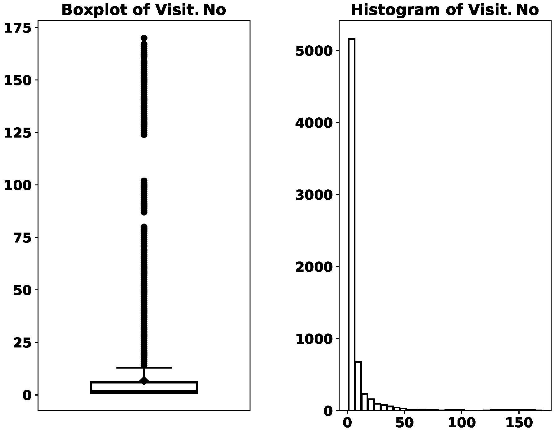
Next, we look at the numerical variables Visit.No and ServTime.
The mean and median of
Visit.No are 6.83 and 2, and the minimum and the maximum are 1 and 170.
Figure 1 visualizes
Visit.No’s distribution. It is highly skewed to the right. While the majority of the records have their
, there are more than 1000 records that have their
. This means that a sizable amount of consultation records come from recurrent consultations for the same medical condition.
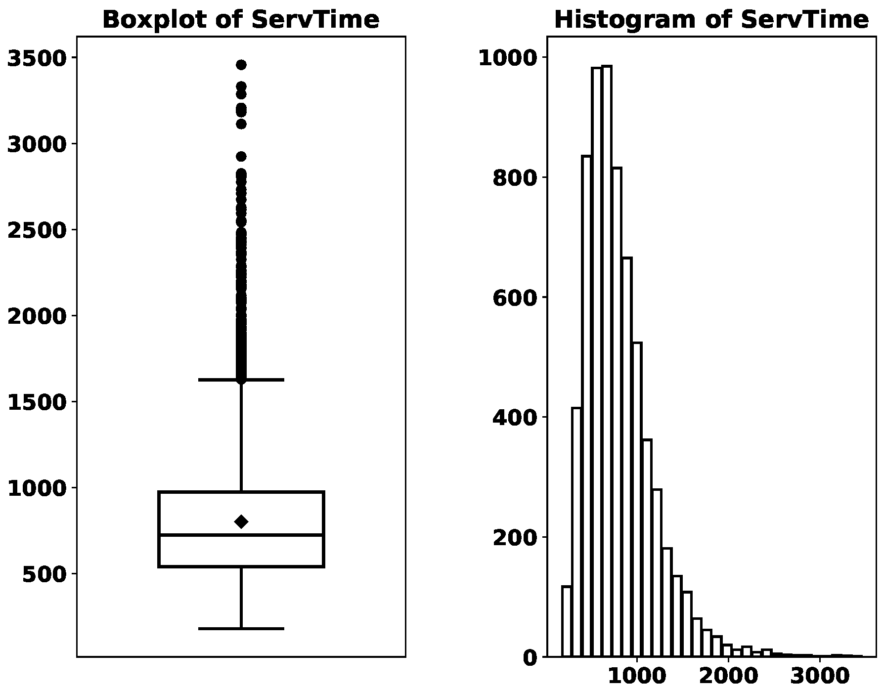
The distribution of
ServTime can be found in
Figure 2. The boxplot shows that its mean (a dot above the median line) is slightly larger than its median, and the distribution is moderately skewed to the right. While it is fairly common in the appointment scheduling literature that the service time is assumed to be exponentially distributed [
17,
18,
34], the histogram in
Figure 2 suggests otherwise, at least in the outpatient clinic in question. It will be interesting and value-adding to test the performance of those methods, developed under stylized assumptions, using realistic datasets such as ours.
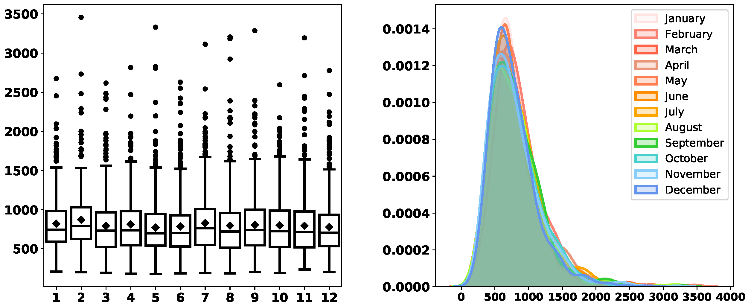
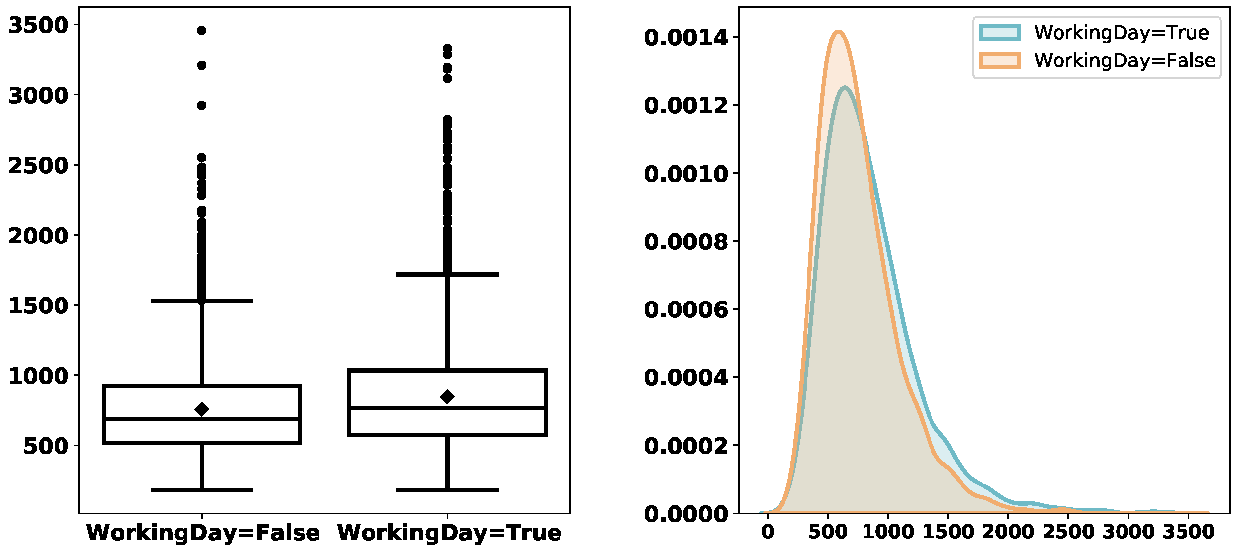
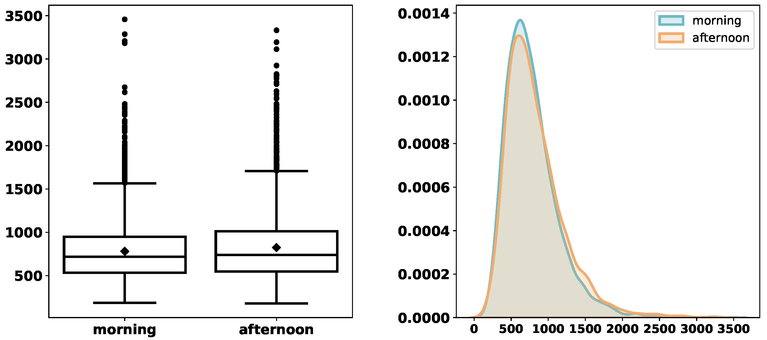
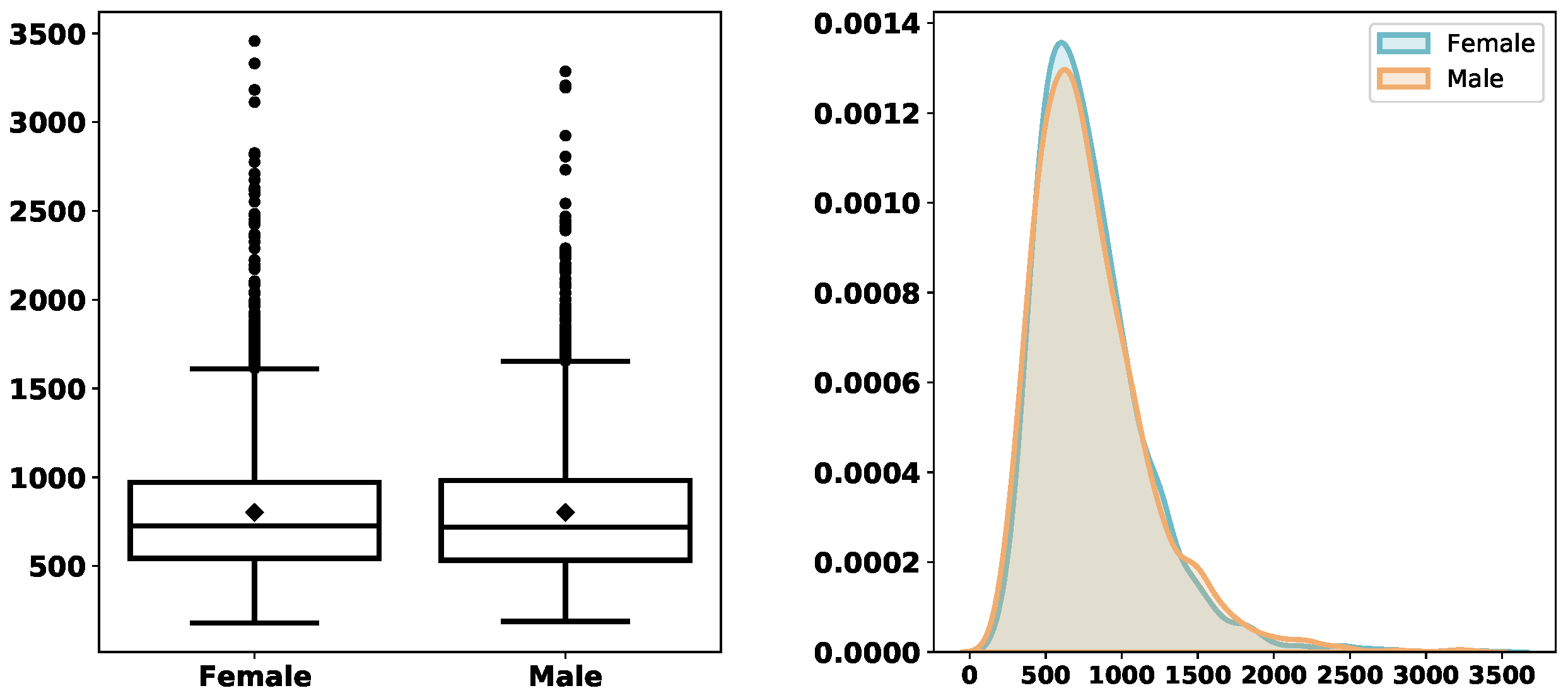
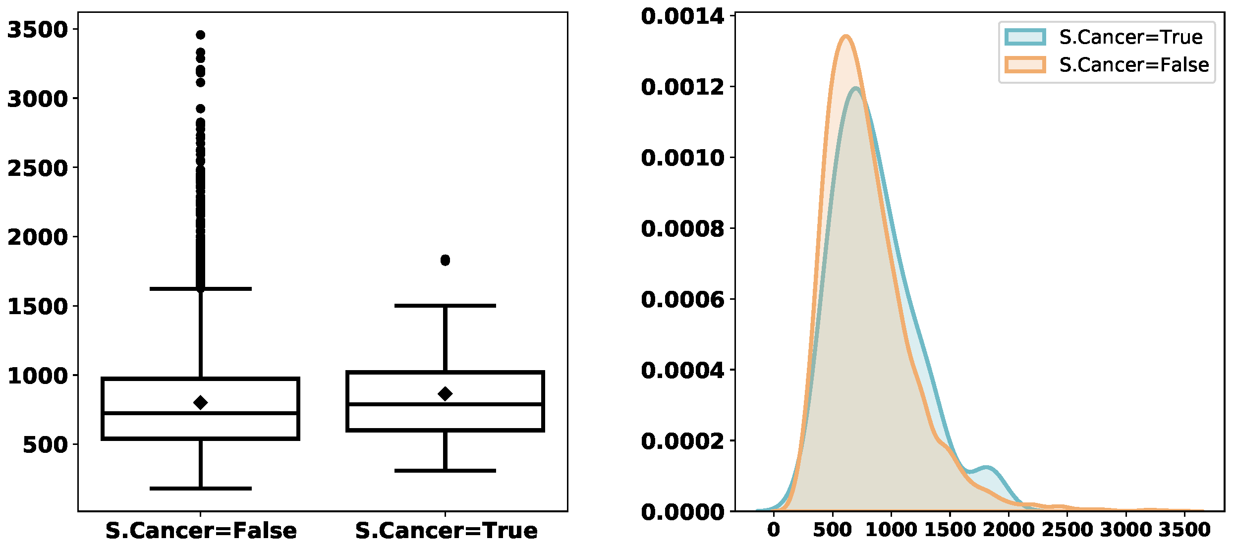
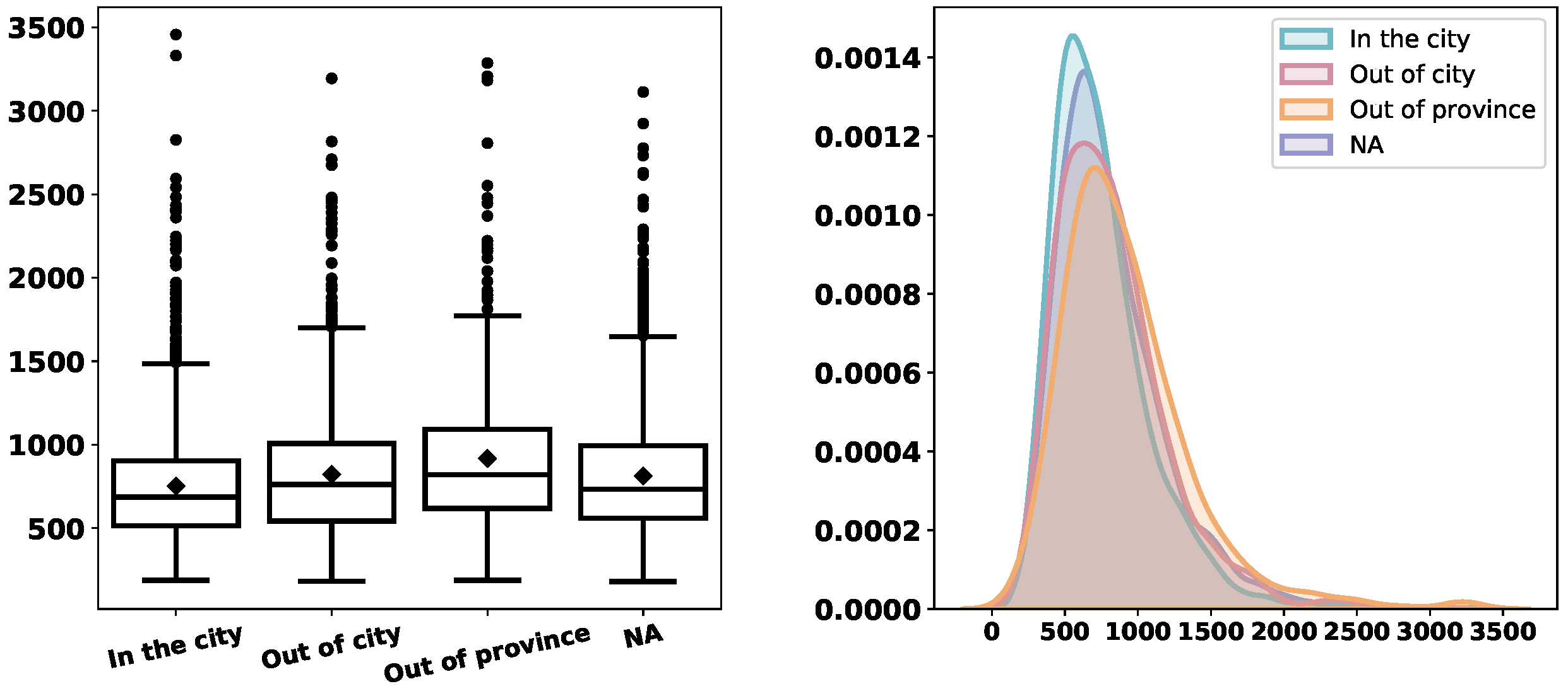
We are interested in the service times and informative characteristics distinguishing them. Therefore, we explore the distribution of
ServTime grouped by different categorical/logical variables.
Figure 3,
Figure 4,
Figure 5,
Figure 6,
Figure 7,
Figure 8 and
Figure 9 depict the derived service-time distributions grouped by
Month,
WorkingDay,
AM_PM,
Gender,
M.Cancer,
S.Cancer, and
Address, respectively. From these figures, we can find that they have noticeable effects on the distributions of
ServTime.
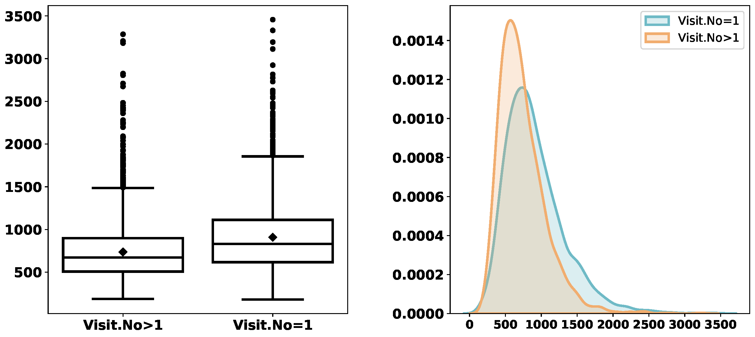
Extant studies constantly find that the service time of a first-time visit and that of a follow-up one follow different distributions. Hence, we explore the distribution of
ServTime based on whether
Visit.No is equal to 1 or not. This essentially converts
Visit.No into a logical variable whose value depends on whether
Visit.No is equal to 1.
Figure 10 illustrates that first-time visits overall take a longer service time.
Table 5 further compares the
ServTime of
and that of
with different grouping. Overall, both means and medians of
ServTime are larger in the case of
, no matter which categorical variable is used for grouping.
Lastly, we regress
ServTime on the rest of the variables.
Table 6 summarizes the regression result. The coefficients of
Visit.No,
M.Cancer,
Address, and
AM_PM are statistically significant at the
level of significance. The coefficient of
Visit.No is
. This means that an extra previous visit for the same condition, on average, reduces the service time by
seconds. The coefficient of
M.Cancer is
. This means that consultations mainly for cancer on average are
seconds longer than those mainly not for cancer.
Address is a factor with four levels: {‘In the city’, ‘Out of city’, ‘Out of province’, and ‘NA’}. ‘In the city’ is the baseline. The regression result suggests that the consultation of a patient with no address provided, on average, takes
seconds more than the baseline; the consultation of a patient from outside of the city but within the province, on average, takes
seconds more than the baseline; and the consultation of a patient from another province, on average, takes
seconds more than the baseline. The
Address variable may be related to customer loyalty or illness severity. An intuitive interpretation is that a patient is unlikely to travel a long distance to consult for some minor health issue. The coefficient of
AM_PM_morning is
. This suggests that, if other things are equal, on average, a consultation in the morning is
seconds shorter than its afternoon counterpart. Of course, all these interpretations are based on the linear regression model. Future users of the data should conduct a more comprehensive analysis to gain more insights.


