
Wave-Encoded Model-Based Deep Learning for Highly Accelerated Imaging with Joint Reconstruction
 , , , , ,
Abstract
:
1. Introduction
2. Theory
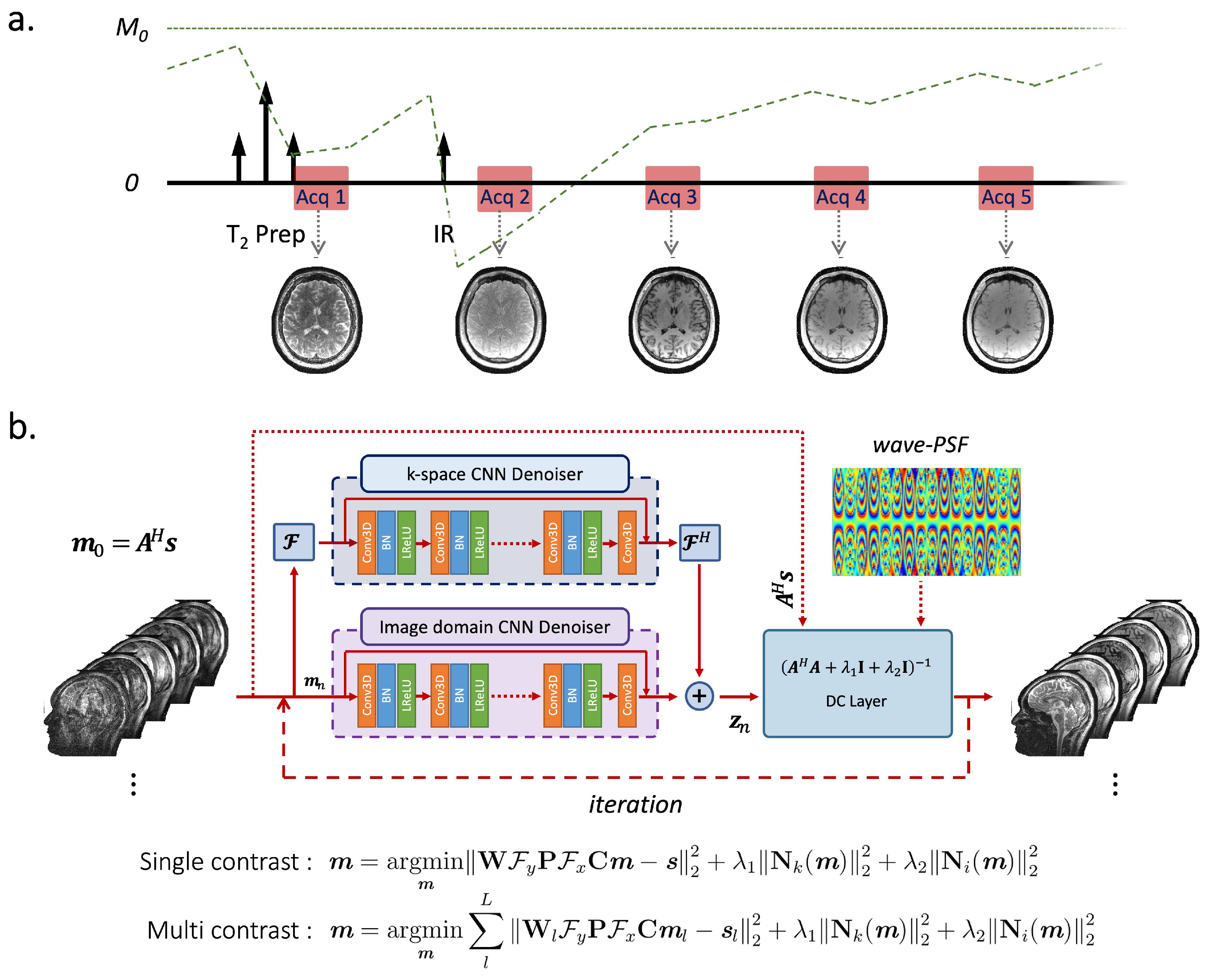
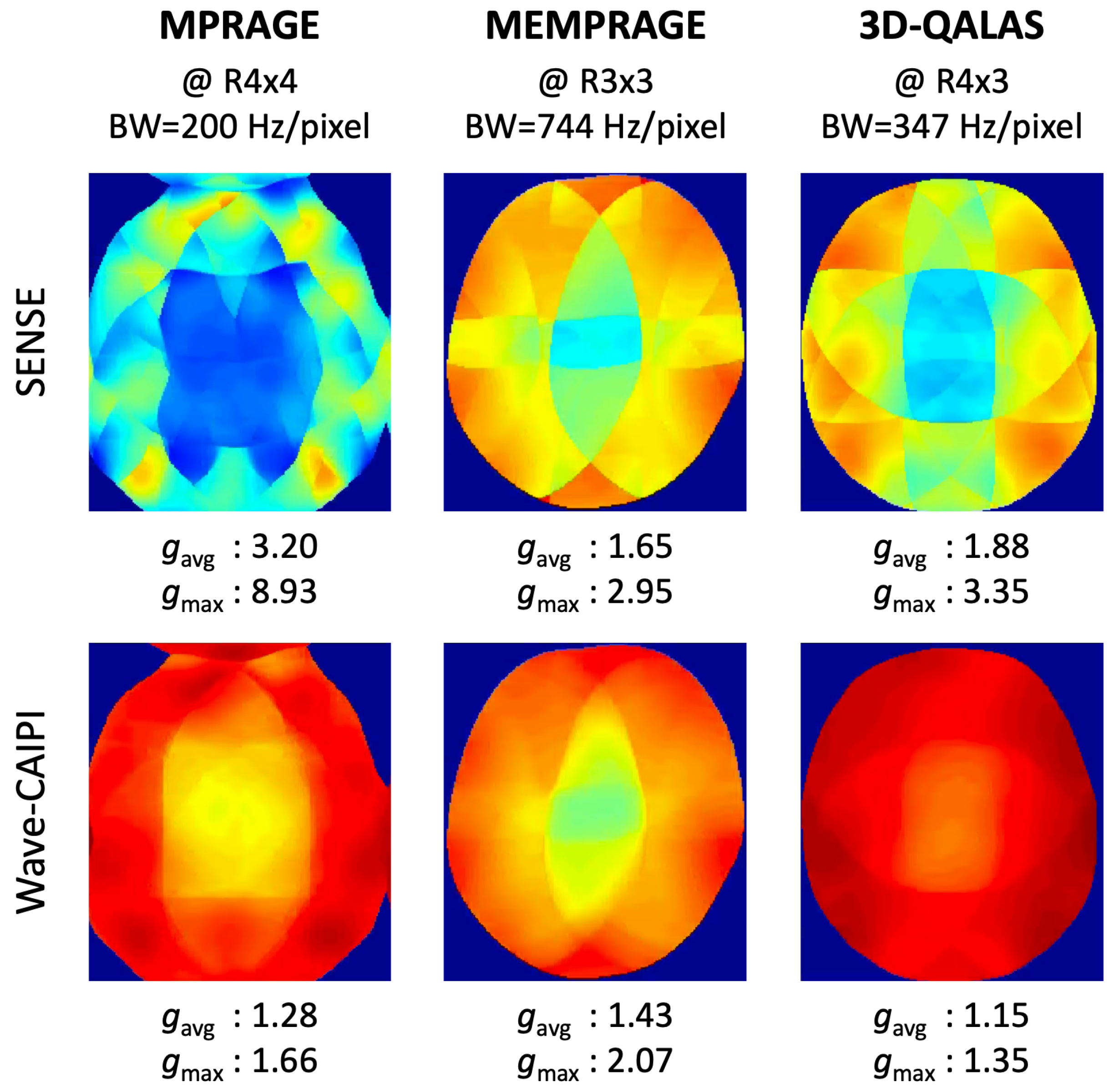
2.1. Wave-CAIPI
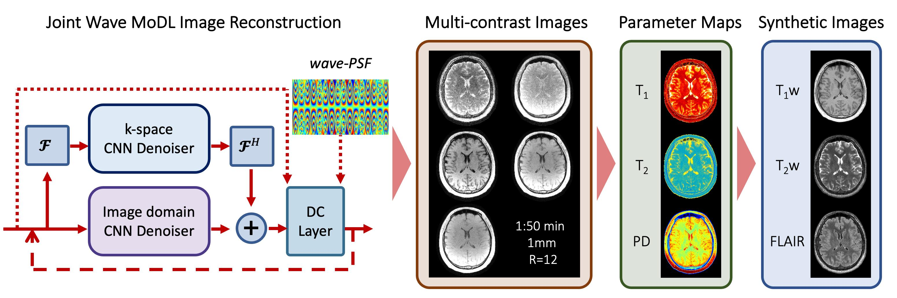
2.2. 3D-QALAS
3. Methods
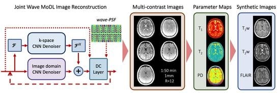
3.1. Wave-MoDL
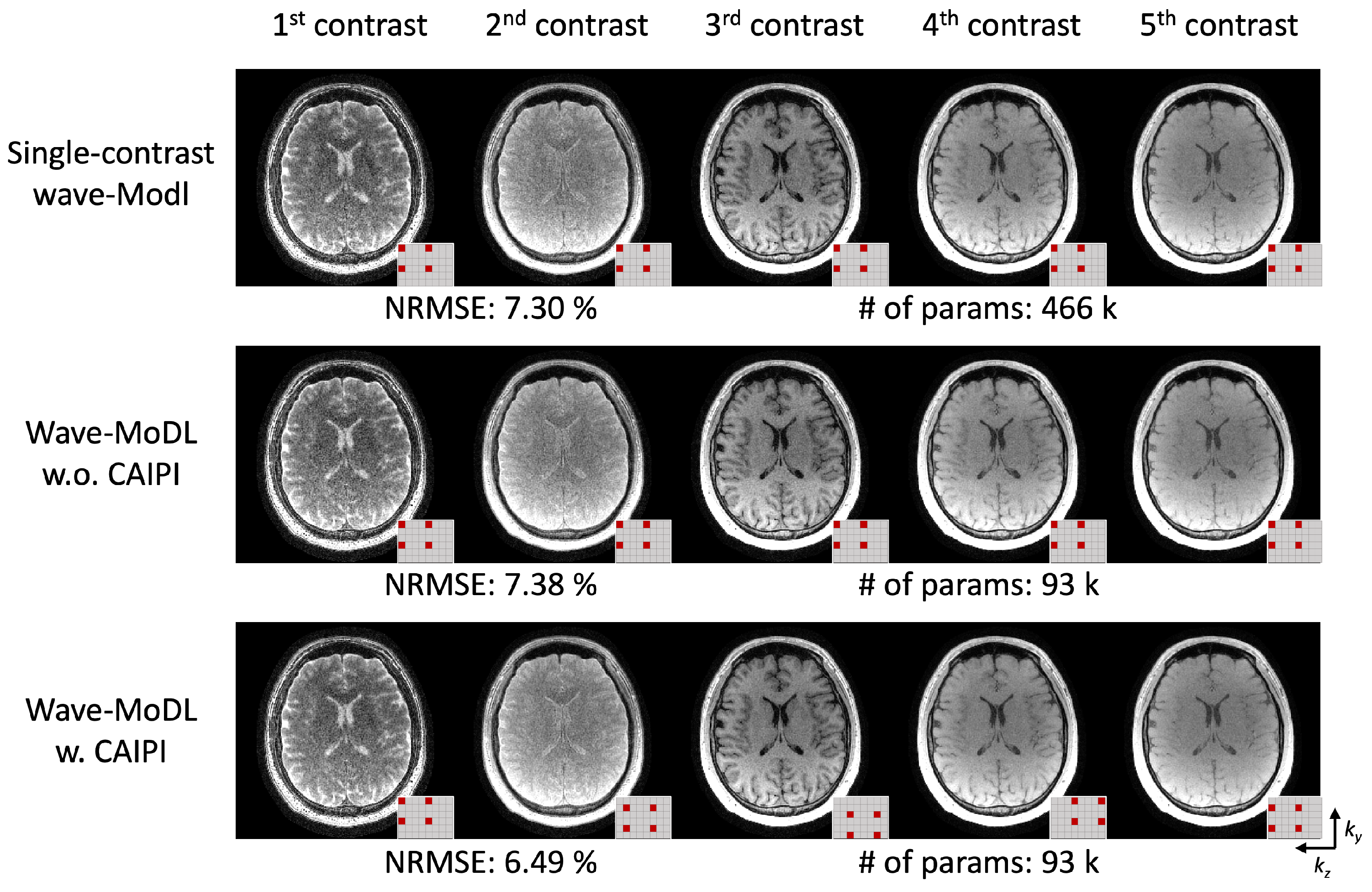
3.2. Wave-MoDL for Multicontrast Image Reconstruction
3.3. Experiments
3.3.1. MPRAGE Database
3.3.2. MEMPRAGE Database
3.3.3. 3D-QALAS Database
4. Results
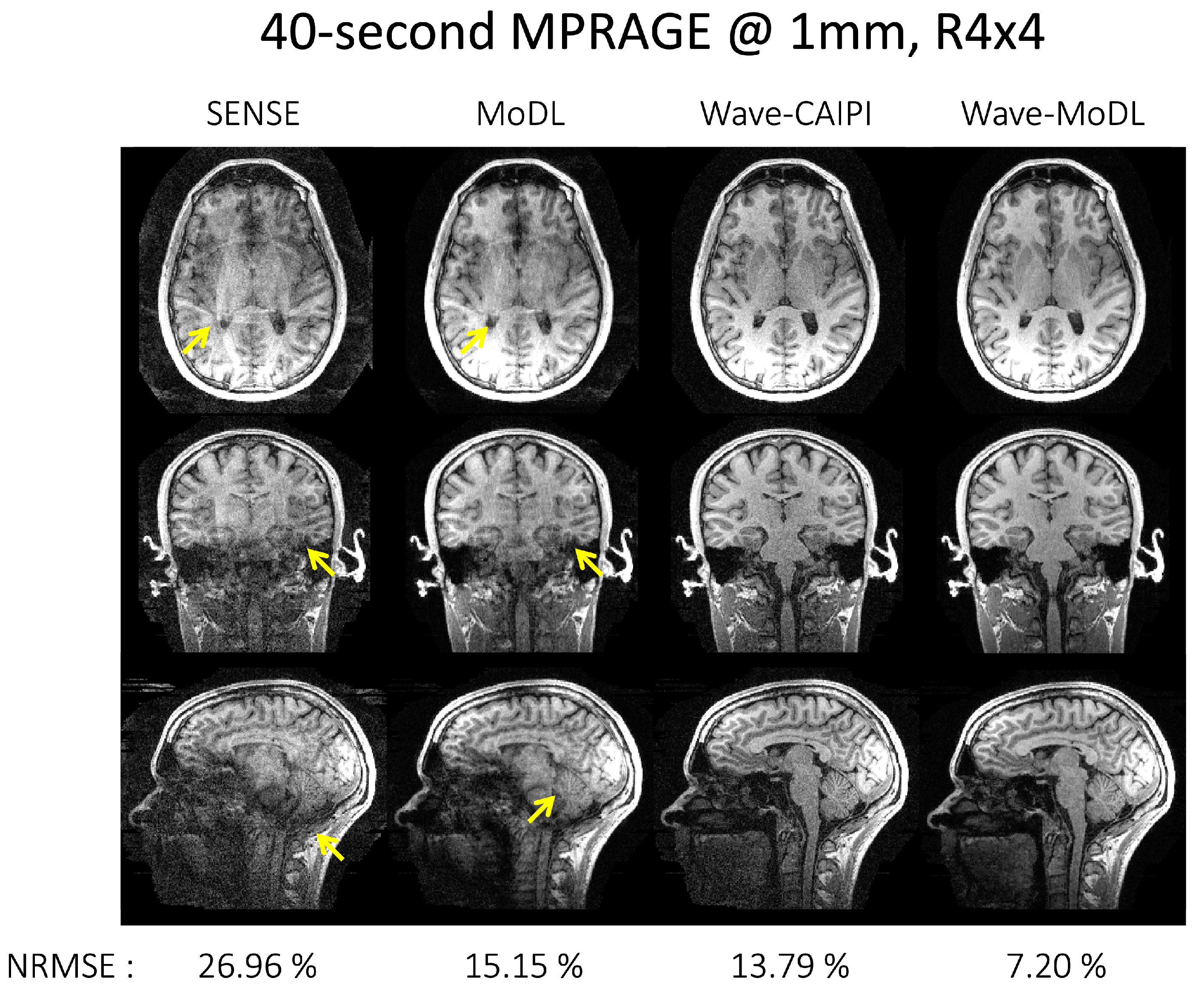
4.1. MPRAGE at R = 4 × 4
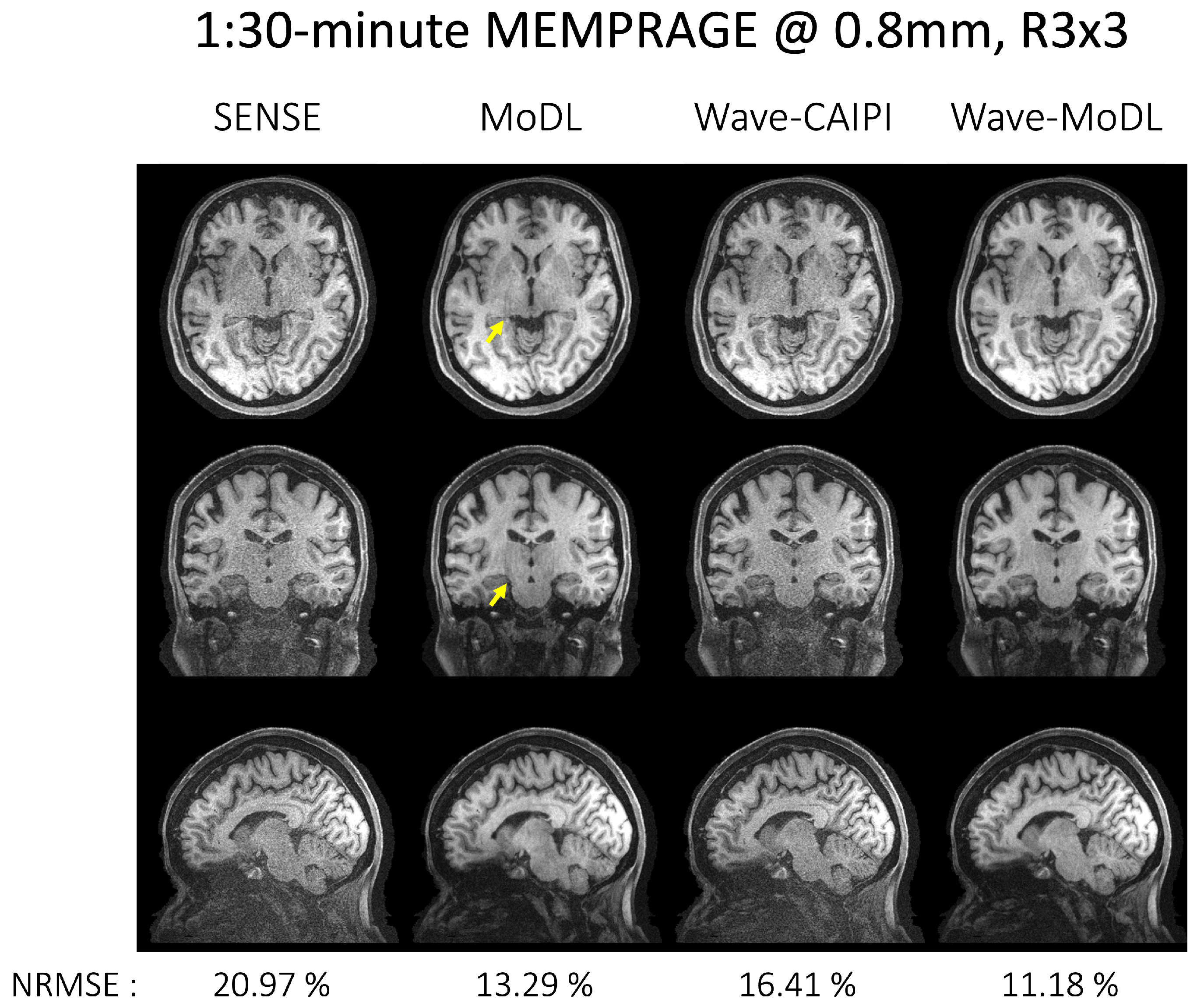
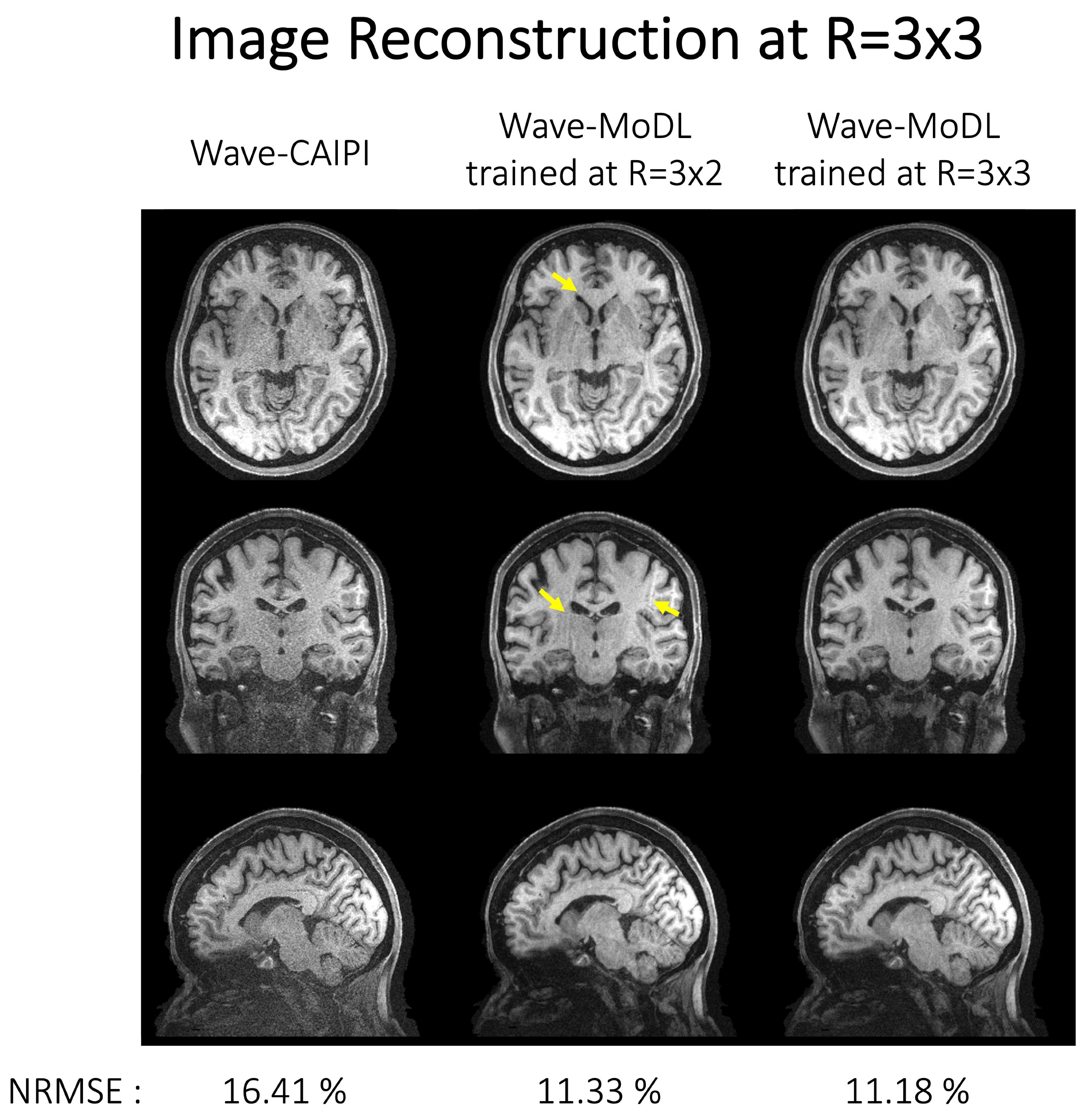
4.2. MEMPRAGE at R = 3 × 3
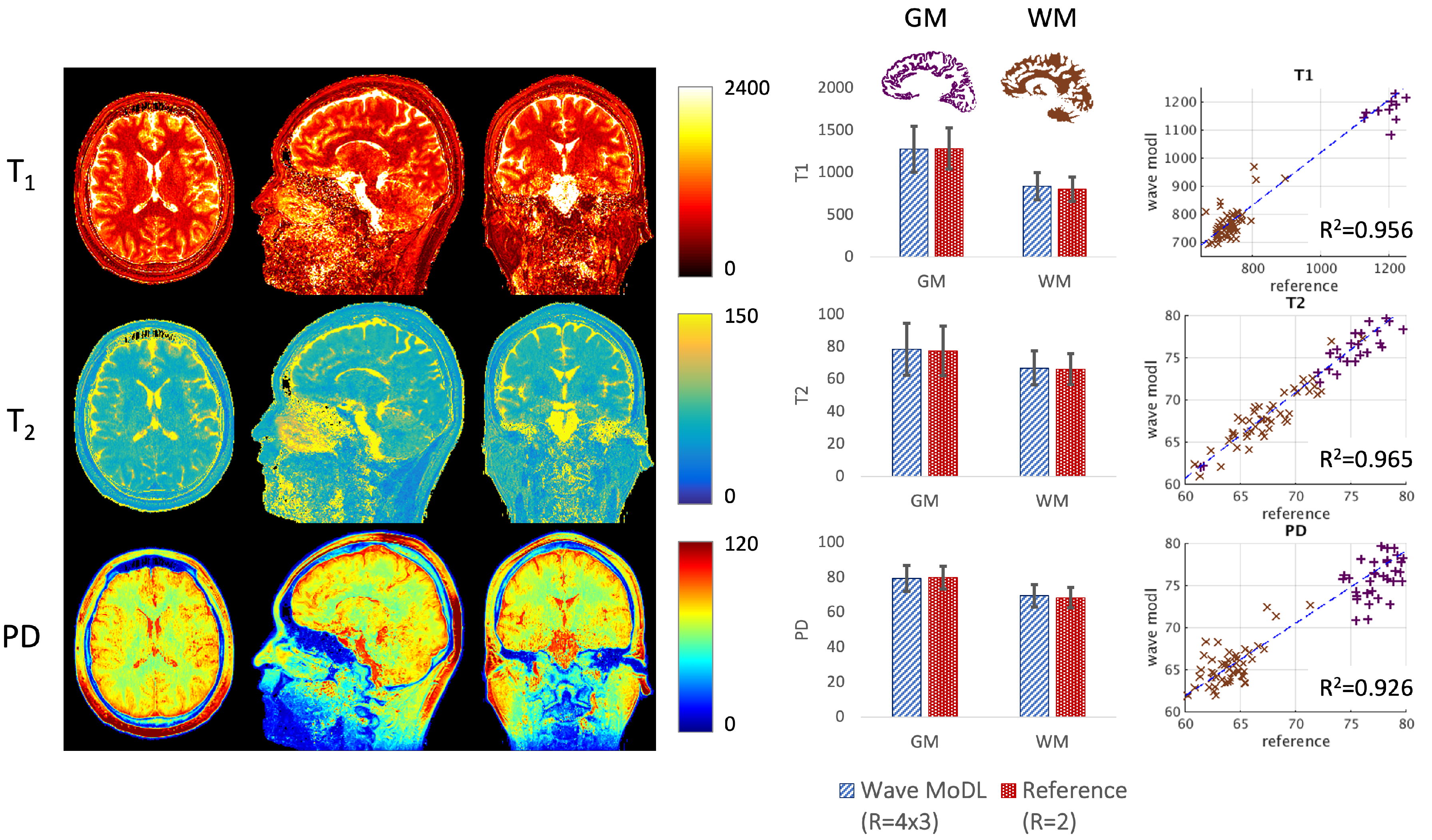
4.3. 3D-QALAS at R = 4 × 3
5. Discussion
6. Conclusions
Supplementary Materials
Author Contributions
Funding
Institutional Review Board Statement
Informed Consent Statement
Data Availability Statement
Acknowledgments
Conflicts of Interest
References
- Nishimura, D.G. Principles of Magnetic Resonance Imaging; Stanford University: Stanford, CA, USA, 1996. [Google Scholar]
- Pruessmann, K.P.; Weiger, M.; Scheidegger, M.B.; Boesiger, P. SENSE: Sensitivity encoding for fast MRI. Magn. Reson. Med. Off. J. Int. Soc. Magn. Reson. Med. 1999, 42, 952–962. [Google Scholar] [CrossRef]
- Griswold, M.A.; Jakob, P.M.; Heidemann, R.M.; Nittka, M.; Jellus, V.; Wang, J.; Kiefer, B.; Haase, A. Generalized autocalibrating partially parallel acquisitions (GRAPPA). Magn. Reson. Med. 2002, 47, 1202–1210. [Google Scholar] [CrossRef] [PubMed] [Green Version]
- Uecker, M.; Lai, P.; Murphy, M.J.; Virtue, P.; Elad, M.; Pauly, J.M.; Vasanawala, S.S.; Lustig, M. ESPIRiT—An eigenvalue approach to autocalibrating parallel MRI: Where SENSE meets GRAPPA. Magn. Reson. Med. 2014, 71, 990–1001. [Google Scholar] [CrossRef] [PubMed] [Green Version]
- Breuer, F.A.; Blaimer, M.; Heidemann, R.M.; Mueller, M.F.; Griswold, M.A.; Jakob, P.M. Controlled aliasing in parallel imaging results in higher acceleration (CAIPIRINHA) for multi-slice imaging. Magn. Reson. Med. 2005, 53, 684–691. [Google Scholar] [CrossRef]
- Breuer, F.A.; Blaimer, M.; Mueller, M.F.; Seiberlich, N.; Heidemann, R.M.; Griswold, M.A.; Jakob, P.M. Controlled aliasing in volumetric parallel imaging (2D CAIPIRINHA). Magn. Reson. Med. 2006, 55, 549–556. [Google Scholar] [CrossRef] [PubMed]
- Bilgic, B.; Gagoski, B.A.; Cauley, S.F.; Fan, A.P.; Polimeni, J.R.; Grant, P.E.; Wald, L.L.; Setsompop, K. Wave-CAIPI for highly accelerated 3D imaging. Magn. Reson. Med. 2015, 73, 2152–2162. [Google Scholar] [CrossRef] [PubMed] [Green Version]
- Gagoski, B.A.; Bilgic, B.; Eichner, C.; Bhat, H.; Grant, P.E.; Wald, L.L.; Setsompop, K. RARE/turbo spin echo imaging with simultaneous multislice Wave-CAIPI: RARE/TSE with SMS Wave-CAIPI. Magn. Reson. Med. 2015, 73, 929–938. [Google Scholar] [CrossRef] [Green Version]
- Chen, F.; Taviani, V.; Tamir, J.I.; Cheng, J.Y.; Zhang, T.; Song, Q.; Hargreaves, B.A.; Pauly, J.M.; Vasanawala, S.S. Self-calibrating wave-encoded variable-density single-shot fast spin echo imaging. J. Magn. Reson. Imaging 2018, 47, 954–966. [Google Scholar] [CrossRef] [PubMed]
- Polak, D.; Setsompop, K.; Cauley, S.F.; Gagoski, B.A.; Bhat, H.; Maier, F.; Bachert, P.; Wald, L.L.; Bilgic, B. Wave-CAIPI for highly accelerated MP-RAGE imaging. Magn. Reson. Med. 2018, 79, 401–406. [Google Scholar] [CrossRef]
- Kim, T.H.; Bilgic, B.; Polak, D.; Setsompop, K.; Haldar, J.P. Wave-LORAKS: Combining wave encoding with structured low-rank matrix modeling for more highly accelerated 3D imaging. Magn. Reson. Med. 2019, 81, 1620–1633. [Google Scholar] [CrossRef] [PubMed]
- Cho, J.; Liao, C.; Tian, Q.; Zhang, Z.; Xu, J.; Lo, W.C.; Poser, B.A.; Stenger, V.A.; Stockmann, J.; Setsompop, K. Highly accelerated EPI with wave encoding and multi-shot simultaneous multislice imaging. Magn. Reson. Med. 2022, 88, 1180–1197. [Google Scholar] [CrossRef]
- Lustig, M.; Donoho, D.; Pauly, J.M. Sparse MRI: The application of compressed sensing for rapid MR imaging. Magn. Reson. Med. Off. J. Int. Soc. Magn. Reson. Med. 2007, 58, 1182–1195. [Google Scholar] [CrossRef] [PubMed]
- Lustig, M.; Donoho, D.L.; Santos, J.M.; Pauly, J.M. Compressed sensing MRI. IEEE Signal Process. Mag. 2008, 25, 72–82. [Google Scholar] [CrossRef]
- Haldar, J.P. Low-rank modeling of local k-space neighborhoods (LORAKS) for constrained MRI. IEEE Trans. Med. Imaging 2013, 33, 668–681. [Google Scholar] [CrossRef] [PubMed] [Green Version]
- Shin, P.J.; Larson, P.E.; Ohliger, M.A.; Elad, M.; Pauly, J.M.; Vigneron, D.B.; Lustig, M. Calibrationless parallel imaging reconstruction based on structured low-rank matrix completion. Magn. Reson. Med. 2014, 72, 959–970. [Google Scholar] [CrossRef] [PubMed] [Green Version]
- Jin, K.H.; Lee, D.; Ye, J.C. A general framework for compressed sensing and parallel MRI using annihilating filter based low-rank Hankel matrix. IEEE Trans. Comput. Imaging 2016, 2, 480–495. [Google Scholar] [CrossRef] [Green Version]
- Mani, M.; Jacob, M.; Kelley, D.; Magnotta, V. Multi-shot sensitivity-encoded diffusion data recovery using structured low-rank matrix completion (MUSSELS): Annihilating Filter K-Space Formulation for Multi-Shot DWI Recovery. Magn. Reson. Med. 2017, 78, 494–507. [Google Scholar] [CrossRef] [PubMed] [Green Version]
- Lustig, M.; Pauly, J.M. SPIRiT: Iterative self-consistent parallel imaging reconstruction from arbitrary k-space. Magn. Reson. Med. 2010, 64, 457–471. [Google Scholar] [CrossRef] [PubMed] [Green Version]
- Murphy, M.; Alley, M.; Demmel, J.; Keutzer, K.; Vasanawala, S.; Lustig, M. Fast ℓ1-SPIRiT compressed sensing parallel imaging MRI: Scalable parallel implementation and clinically feasible runtime. IEEE Trans. Med. Imaging 2012, 31, 1250–1262. [Google Scholar] [CrossRef] [PubMed] [Green Version]
- Ongie, G.; Jacob, M. Off-the-grid recovery of piecewise constant images from few Fourier samples. SIAM J. Imaging Sci. 2016, 9, 1004–1041. [Google Scholar] [CrossRef] [PubMed]
- Haldar, J.P.; Zhuo, J. P-LORAKS: Low-rank modeling of local k-space neighborhoods with parallel imaging data. Magn. Reson. Med. 2016, 75, 1499–1514. [Google Scholar] [CrossRef] [PubMed] [Green Version]
- Kwon, K.; Kim, D.; Park, H. A parallel MR imaging method using multilayer perceptron. Med. Phys. 2017, 44, 6209–6224. [Google Scholar] [CrossRef] [PubMed] [Green Version]
- Hammernik, K.; Klatzer, T.; Kobler, E.; Recht, M.P.; Sodickson, D.K.; Pock, T.; Knoll, F. Learning a variational network for reconstruction of accelerated MRI data: Learning a Variational Network for Reconstruction of Accelerated MRI Data. Magn. Reson. Med. 2018, 79, 3055–3071. [Google Scholar] [CrossRef]
- Han, Y.; Sunwoo, L.; Ye, J.C. k-Space Deep Learning for Accelerated MRI. IEEE Trans. Med. Imaging 2020, 39, 377–386. [Google Scholar] [CrossRef] [PubMed] [Green Version]
- Eo, T.; Jun, Y.; Kim, T.; Jang, J.; Lee, H.J.; Hwang, D. KIKI-net: Cross-domain convolutional neural networks for reconstructing undersampled magnetic resonance images. Magn. Reson. Med. 2018, 80, 2188–2201. [Google Scholar] [CrossRef] [PubMed]
- Akçakaya, M.; Moeller, S.; Weingärtner, S.; Uğurbil, K. Scan-specific robust artificial-neural-networks for k-space interpolation (RAKI) reconstruction: Database-free deep learning for fast imaging. Magn. Reson. Med. 2019, 81, 439–453. [Google Scholar] [CrossRef] [Green Version]
- Kim, T.H.; Garg, P.; Haldar, J.P. LORAKI: Autocalibrated Recurrent Neural Networks for Autoregressive MRI Reconstruction in k-Space. arXiv 2019, arXiv:1904.09390. [Google Scholar]
- Polak, D.; Cauley, S.; Bilgic, B.; Gong, E.; Bachert, P.; Adalsteinsson, E.; Setsompop, K. Joint multi-contrast variational network reconstruction (jVN) with application to rapid 2D and 3D imaging. Magn. Reson. Med. 2020, 84, 1456–1469. [Google Scholar] [CrossRef] [Green Version]
- Beker, O.; Liao, C.; Cho, J.; Zhang, Z.; Setsompop, K.; Bilgic, B. Scan-specific, Parameter-free Artifact Reduction in K-space (SPARK). arXiv 2019, arXiv:1911.07219. [Google Scholar]
- Arefeen, Y.; Beker, O.; Cho, J.; Yu, H.; Adalsteinsson, E.; Bilgic, B. Scan-specific artifact reduction in k-space (SPARK) neural networks synergize with physics-based reconstruction to accelerate MRI. Magn. Reson. Med. 2022, 87, 764–780. [Google Scholar] [CrossRef] [PubMed]
- Aggarwal, H.K.; Mani, M.P.; Jacob, M. MoDL: Model Based Deep Learning Architecture for Inverse Problems. IEEE Trans. Med. Imaging 2018, 38, 394–405. [Google Scholar] [CrossRef] [PubMed]
- Aggarwal, H.K.; Mani, M.P.; Jacob, M. MoDL-MUSSELS: Model-Based Deep Learning for Multi-Shot Sensitivity Encoded Diffusion MRI. IEEE Trans. Med. Imaging 2020, 39, 1268–1277. [Google Scholar] [CrossRef] [PubMed]
- Seiler, A.; Nöth, U.; Hok, P.; Reiländer, A.; Maiworm, M.; Baudrexel, S.; Meuth, S.; Rosenow, F.; Steinmetz, H.; Wagner, M.; et al. Multiparametric quantitative MRI in neurological diseases. Front. Neurol. 2021, 12, 640239. [Google Scholar] [CrossRef] [PubMed]
- Kvernby, S.; Warntjes, M.J.B.; Haraldsson, H.; Carlhäll, C.J.; Engvall, J.; Ebbers, T. Simultaneous three-dimensional myocardial T1 and T2 mapping in one breath hold with 3D-QALAS. J. Cardiovasc. Magn. Reson. 2014, 16, 102. [Google Scholar] [CrossRef] [Green Version]
- Kvernby, S.; Warntjes, M.; Engvall, J.; Carlhäll, C.J.; Ebbers, T. Clinical feasibility of 3D-QALAS – Single breath-hold 3D myocardial T1- and T2-mapping. Magn. Reson. Imaging 2017, 38, 13–20. [Google Scholar] [CrossRef]
- Fujita, S.; Hagiwara, A.; Hori, M.; Warntjes, M.; Kamagata, K.; Fukunaga, I.; Andica, C.; Maekawa, T.; Irie, R. Three-dimensional high-resolution simultaneous quantitative mapping of the whole brain with 3D-QALAS: An accuracy and repeatability study. Magn. Reson. Imaging 2019, 63, 235–243. [Google Scholar] [CrossRef]
- Fujita, S.; Hagiwara, A.; Takei, N.; Hwang, K.P.; Fukunaga, I.; Kato, S.; Andica, C.; Kamagata, K.; Yokoyama, K.; Hattori, N.; et al. Accelerated Isotropic Multiparametric Imaging by High Spatial Resolution 3D-QALAS With Compressed Sensing: A Phantom, Volunteer, and Patient Study. Investig. Radiol. 2021, 56, 292–300. [Google Scholar] [CrossRef]
- Cho, J.; Tian, Q.; Frost, R.; Chatnuntawech, I.; Bilgic, B. Wave-encoded model-based deep learning with joint reconstruction and segmentation. In Proceedings of the 29th Scientific Meeting of ISMRM, Online Conference, 15–20 May 2021; p. 1982. [Google Scholar]
- Van der Kouwe, A.J.; Benner, T.; Salat, D.H.; Fischl, B. Brain morphometry with multiecho MPRAGE. Neuroimage 2008, 40, 559–569. [Google Scholar] [CrossRef] [Green Version]
- Dale, A.M.; Fischl, B.; Sereno, M.I. Cortical Surface-Based Analysis: I. Segmentation and Surface Reconstruction. Neuroimage 1999, 9, 179–194. [Google Scholar] [CrossRef]
- Desikan, R.S.; Ségonne, F.; Fischl, B.; Quinn, B.T.; Dickerson, B.C.; Blacker, D.; Buckner, R.L.; Dale, A.M.; Maguire, R.P.; Hyman, B.T. An automated labeling system for subdividing the human cerebral cortex on MRI scans into gyral based regions of interest. Neuroimage 2006, 31, 968–980. [Google Scholar] [CrossRef]
- Polak, D.; Cauley, S.; Huang, S.Y.; Longo, M.G.; Conklin, J.; Bilgic, B.; Ohringer, N.; Raithel, E.; Bachert, P.; Wald, L.L.; et al. Highly-accelerated volumetric brain examination using optimized wave-CAIPI encoding. J. Magn. Reson. Imaging 2019, 50, 961–974. [Google Scholar] [CrossRef] [PubMed]
- Bilgic, B.; Kim, T.H.; Liao, C.; Manhard, M.K.; Wald, L.L.; Haldar, J.P.; Setsompop, K. Improving parallel imaging by jointly reconstructing multi-contrast data. Magn. Reson. Med. 2018, 80, 619–632. [Google Scholar] [CrossRef] [PubMed]
- Frost, R.; Tisdall, M.D.; Hoffmann, M.; Fischl, B.; Salat, D.; van der Kouwe, A.J. Scan-specific assessment of vNav motion artifact mitigation in the HCP Aging study using reverse motion correction. In Proceedings of the 28th Annual Meeting of the International Society of Magnetic Resonance in Medicine, Online Conference, 8–14 August 2020. [Google Scholar]
- Yaman, B.; Hosseini, S.A.H.; Moeller, S.; Ellermann, J.; Uğurbil, K.; Akçakaya, M. Self-supervised learning of physics-guided reconstruction neural networks without fully sampled reference data. Magn. Reson. Med. 2020, 84, 3172–3191. [Google Scholar] [CrossRef] [PubMed]
- Muckley, M.J.; Riemenschneider, B.; Radmanesh, A.; Kim, S.; Jeong, G.; Ko, J.; Jun, Y.; Shin, H.; Hwang, D.; Mostapha, M. Results of the 2020 fastmri challenge for machine learning mr image reconstruction. IEEE Trans. Med. Imaging 2021, 40, 2306–2317. [Google Scholar] [CrossRef] [PubMed]


| MPRAGE | MEMPRAGE | QALAS | |
|---|---|---|---|
| Imaging plane | Sagittal | Sagittal | Sagittal |
| Voxel size [mm3] | |||
| FOV [mm3] | |||
| TR [ms] | 2500 | 2500 | 4500 |
| TI [ms] | 1100 | 1000 | -/100/1000/1900/2700 |
| TE [ms] | 2.28 | 1.81/3.60/5.39/7.18 | 2.35 |
| Receiver bandwidth | 200 Hz/pixel | 744 Hz/pixel | 347 Hz/pixel |
| Maximum wave gradient | 8.80 mT/m | 9.63 mT/m | 16.51 mT/m |
| # of wave cycles | 11 | 4 | 5 |
| Acceleration | |||
| Scan time | 40 s | 1 min 30 s | 1 min 50 s |
| #/depth of hidden layers | 5/24 | 5/24 | 5/24 |
| # of network parameters | 85,974 | 91,458 | 93,286 |
| # of subjects (train/validate/test) | 8/1/1 | 22/4/4 | 8/1/1 |
Publisher’s Note: MDPI stays neutral with regard to jurisdictional claims in published maps and institutional affiliations. |
© 2022 by the authors. Licensee MDPI, Basel, Switzerland. This article is an open access article distributed under the terms and conditions of the Creative Commons Attribution (CC BY) license (https://creativecommons.org/licenses/by/4.0/).
Share and Cite
Cho, J.; Gagoski, B.; Kim, T.H.; Tian, Q.; Frost, R.; Chatnuntawech, I.; Bilgic, B. Wave-Encoded Model-Based Deep Learning for Highly Accelerated Imaging with Joint Reconstruction. Bioengineering 2022, 9, 736. https://doi.org/10.3390/bioengineering9120736
Cho J, Gagoski B, Kim TH, Tian Q, Frost R, Chatnuntawech I, Bilgic B. Wave-Encoded Model-Based Deep Learning for Highly Accelerated Imaging with Joint Reconstruction. Bioengineering. 2022; 9(12):736. https://doi.org/10.3390/bioengineering9120736
Chicago/Turabian StyleCho, Jaejin, Borjan Gagoski, Tae Hyung Kim, Qiyuan Tian, Robert Frost, Itthi Chatnuntawech, and Berkin Bilgic. 2022. "Wave-Encoded Model-Based Deep Learning for Highly Accelerated Imaging with Joint Reconstruction" Bioengineering 9, no. 12: 736. https://doi.org/10.3390/bioengineering9120736