

Assessment of Model Accuracy in Eyes Open and Closed EEG Data: Effect of Data Pre-Processing and Validation Methods

Abstract
:1. Introduction
- that interpersonal variability significantly affects the classification accuracy;
- data preprocessing methods significantly affect the classification accuracy;
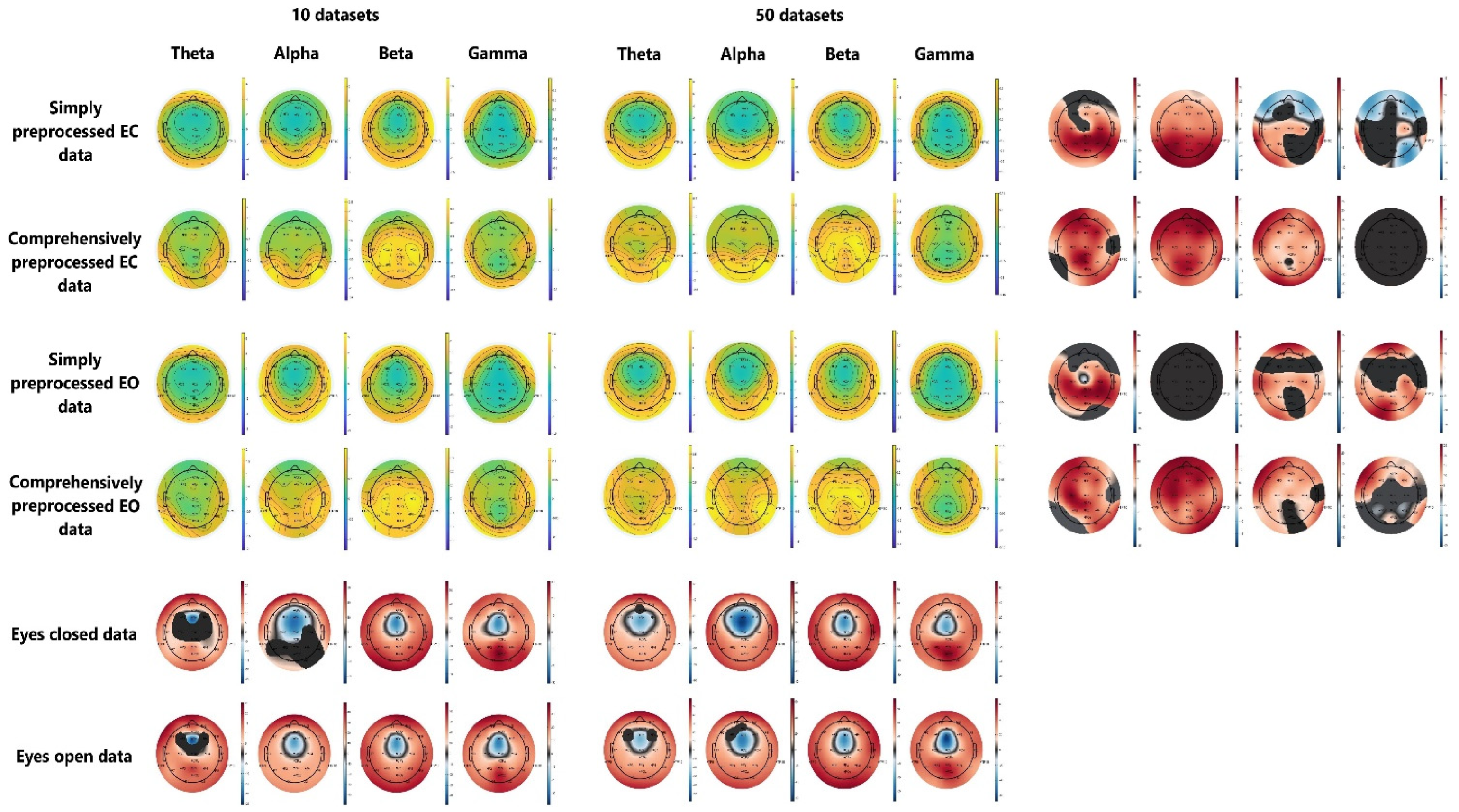
- the resulting frequency-power feature dataset is significantly affected by interpersonal variability and data preprocessing.
2. Materials and Methods
2.1. Data Collection, Preprocessing, Feature Extraction and Dataset Generation
2.1.1. Data Collection
2.1.2. Data Preprocessing
- Visual inspection and rejection of obvious electrode detachment/malfunction and other similar types of artifacts
- Filtering (1–50 Hz)
- Independent component analysis (ICA) decomposition
- Rejection of artifact independent components
- Channel automatic rejection by spectrum, ±3 SD outlier channels removed
- Visual inspection and rejection of any remaining artifact data
- Re-referencing to average
- Blind source separation (BSS) correction of muscle artifacts
- Interpolation of missing channels
- Epoching of the data into 2 s long epochs
- Visual inspection of the dataset to determine the extent of saturation with artifacts by inspecting the data for obvious electrode detachment/malfunction and other similar types of artifacts
- Filtering (1–50 Hz)
- Epoching of the data into 2 s long epochs
- Removal of any epochs where the voltage observed exceeds ±100 μV
2.1.3. Feature Extraction
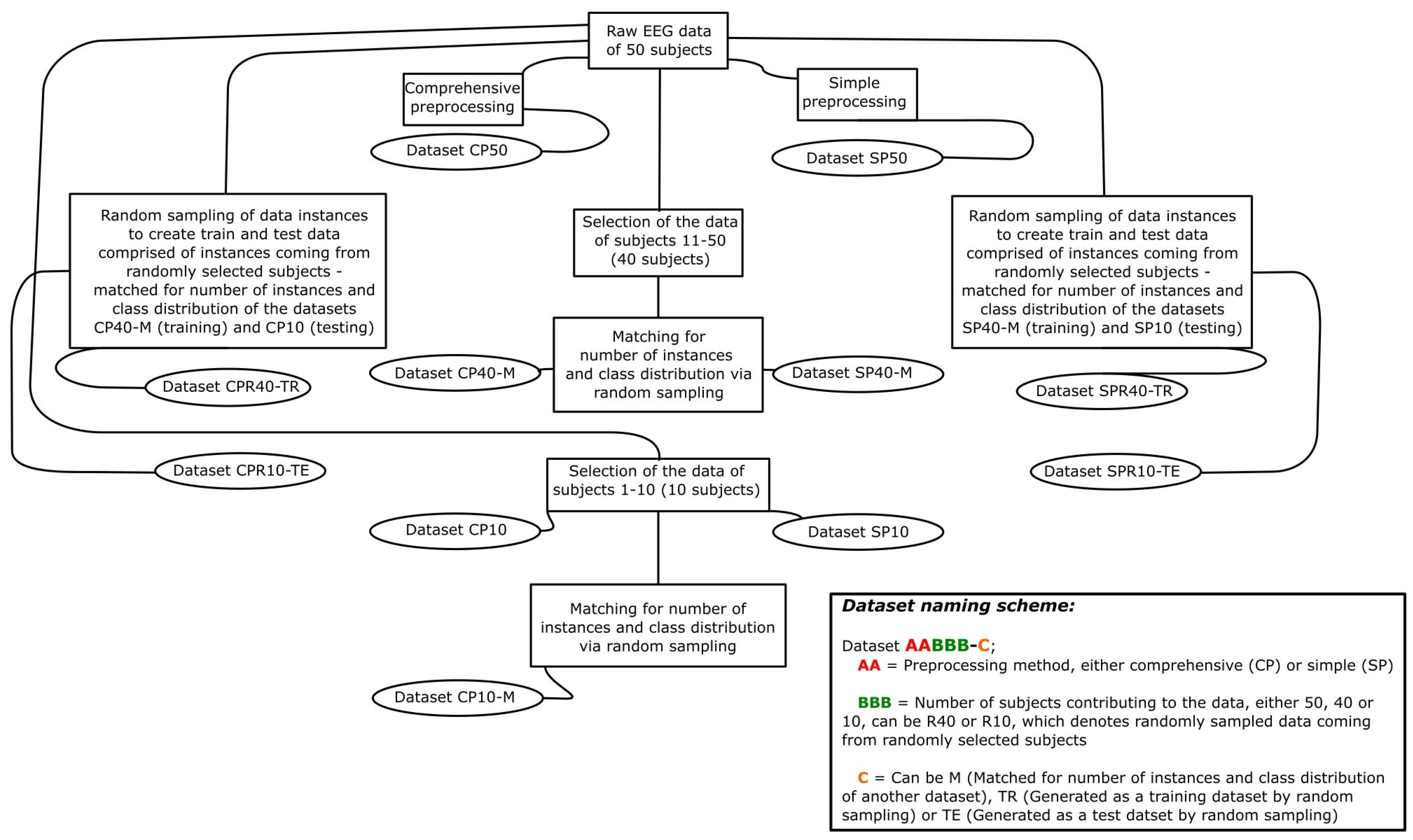
2.1.4. Generated Datasets
2.2. Classification Models
- Rule-based: JRip [26], this classifier implements a propositional rule learner, Repeated Incremental Pruning to Produce Error Reduction (also called RIPPER); PART [27], which unifies the two primary paradigms for rule generating: creating rules from decision trees and the separate-and-conquer rule learning technique by presenting an algorithm for inferring rules through iterative generation of partial decision trees.
- Tree-based: LMT (Logistic Model Trees) [28] classifier for building “logistic model trees”, which are classification trees with logistic regression functions at the leaves; J48 [29] classifier generates a pruned or unpruned decision tree and extract the rules for each path from root to the leave; Random Forest [30], which functions by building a large number of decision trees during the training phase and is an ensemble learning approach for classification, regression, and other tasks. The class that the majority of trees choose in a classification task is the random forest’s output.
- CNN-based models: The Temporal Convolutional Neural network (TCN) follows the work of Bai et al. [31] and consists of two convolutional blocks with 16 convolutional filters of size five each and dilation factors one and two, respectively. Each block contains two sets of dilated causal convolution layers with the same dilation factor, followed by normalization, leackyReLU activation, and spatial dropout layers.
- The Deep Neural Network (DNN) is a simple neural network consisting of three layers: the first layer is a dense layer with 12 units, and “relu” activation; the second layer is 8-unit dense layer (also with “relu” activation); the third layer is 1-unit dense layer with “sigmod” activation.
- Lazy: K-NN (K-Nearest Neighbor) [32], is an instance-based algorithm which selects k (K-NN can select the optimal k based on cross-validation) nearest neighbor and makes a prediction based on their class labels; KStar (instance-based model) [33], is an instance-based classifier, meaning that a test instance’s classification is based on the classification of training instances that are comparable to it as defined by some similarity function (entropy-based distance function).
- Linear models: ANN (Artificial Neural Network) [34], is an adaptable system that picks up new information by using interconnected nodes or neurons in a layered structure that attempts to simulate the structural organization of the human brain. A neural network may be trained to recognize patterns, classify data, and predict future occurrences since it can learn from data; SVM (Support Vector Machine) [34], Logistic Regression [35], classifiers for constructing and applying a multinomial logistic regression model with a ridge estimator.
- Ensemble classifiers: bagged trees and optimized ensemble classifier [32], ensemble classifiers meld results from many weak learners into one high-quality ensemble model.
- Kstar: the global blending parameter was set to 20, and missing values were replaced with average column entropy curves.
- Jrip: the “Pruning” method was applied, the minimum total weight of the instances in a rule was set to 2 and two optimization runs were used;
- PART: the minimum number of instances per rule was 2, a common confidence factor 0.25 was used for pruning and the number of folds to determine the amount of data used for reduced-error pruning was set to 3;
- Logistic Regression: The Ridge value (1 × 10⁻⁸) in the log-likelihood was applied as default;
- LMT: the minimum number of instances at which a node is considered for splitting) was set to 15 and fast regression for using heuristic that avoids cross-validating the number of Logit-Boost iterations at every node was utilized;
- J48: the default confidence factor (0.25) was used for pruning (smaller values incur more pruning. The subtree raising operation was utilized to improve the accuracy when pruning and the minimal number of instances per leaf was put to 2;
- Random Forest: the number of trees in the random forest was set to 100 while the maximum depth of each tree was not limited.
- Optimized Ensemble: the optimized ensemble method of the most successful iteration was AdaBoost, with a maximum of 20 splits, 30 learners and 0.1 learning rate.
- Bagged Trees: the learner type of the model was Decision Tree and the optimal number of split was 6602 with 100 learners;
- K-NN: one neighbor was selected to make a decision and Euclidean metric was used to find the distance;
- SVM: linear function was utilized in kernel mode and “One-vs-One” multiclass method was applied with 1 level of box constraint;
- ANN: the number of fully connected layers (the size of each layer was 10) was set to 3 and “Relu” activation mode was used with 1000 iteration limit.
2.3. Statistics
3. Results
4. Discussion
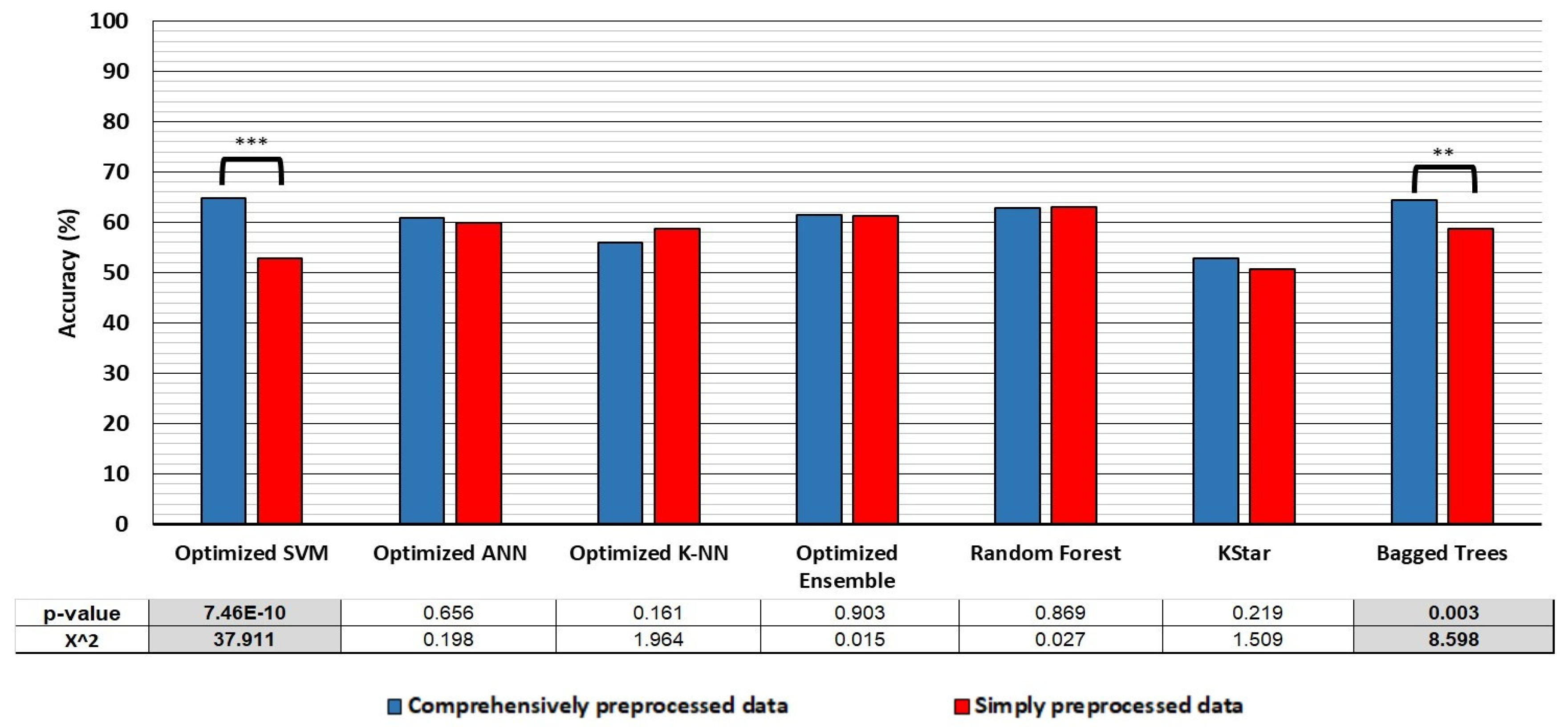
- Classification accuracy: the classifiers trained on simply preprocessed data performed better in the cross-validation, when the compared datasets are balanced for size and class distribution. However, the SVM and Bagged trees algorithms trained on comprehensively preprocessed data performed 12 and 5.7% better, respectively, in hold-out testing, with no differences in accuracy apparent in the cross-validation translating to differences observed in the hold-out accuracy in any of the classifiers.
- Dataset generation: we have found that the EEG data that the classifiers train on differs significantly with regard to the preprocessing methods (and their strictness) used and with dataset sample size. Moreover, we have found that up to 23% more data can be extracted from the raw EEG recordings, when the data is carefully preprocessed.
5. Conclusions and Future Work
Author Contributions
Funding
Institutional Review Board Statement
Data Availability Statement
Acknowledgments
Conflicts of Interest
Appendix A

| Dataset | Accuracy | Precision | Recall | F-Measure | |||
|---|---|---|---|---|---|---|---|
| EO | EC | EO | EC | EO | EC | ||
| Optimized Ensemble | 96.1 | 93.7 | 97.4 | 95.4 | 96.5 | 94.5 | 96.9 |
| Optimized ANN | 93.8 | 91.7 | 95.0 | 91.1 | 95.3 | 91.4 | 95.1 |
| Optimized K-NN | 94.3 | 83.3 | 97.1 | 94.5 | 94.2 | 95.6 | 95.4 |
| Random Forest | 93.5 | 94.6 | 93.0 | 87.0 | 97.2 | 90.6 | 95.0 |
| Optimized SVM | 91.9 | 90.0 | 93.0 | 87.9 | 94.3 | 88.9 | 93.6 |
| Bagged Trees | 92.2 | 85.7 | 96.0 | 92.3 | 92.2 | 88.9 | 94.1 |
| KStar | 91.3 | 89.4 | 92.3 | 86.1 | 94.2 | 87.7 | 93.3 |
| LMT | 88.9 | 85.7 | 90.6 | 83.0 | 92.1 | 84.3 | 91.4 |
| J48 | 86.6 | 80.9 | 89.9 | 82.2 | 89.1 | 81.6 | 89.5 |
| PART | 86.9 | 83.7 | 88.7 | 79.3 | 91.3 | 81.5 | 90.0 |
| Logistic Regression | 86.9 | 82.9 | 89.0 | 80.2 | 90.7 | 81.5 | 89.8 |
| JRip | 86.2 | 80.5 | 89.5 | 81.5 | 88.8 | 81.0 | 89.2 |
| Dataset | Accuracy | Precision | Recall | F-Measure | |||
|---|---|---|---|---|---|---|---|
| EO | EC | EO | EC | EO | EC | ||
| Optimized Ensemble | 98.4 | 98.9 | 97.4 | 98.5 | 98.0 | 98.7 | 97.7 |
| Random Forest | 98.0 | 97.5 | 98.9 | 99.4 | 95.4 | 98.4 | 97.1 |
| Optimized ANN | 96.8 | 97.5 | 95.4 | 97.4 | 95.6 | 97.4 | 95.5 |
| Optimized SVM | 95.9 | 97.8 | 92.6 | 95.9 | 95.9 | 96.8 | 94.2 |
| Bagged Trees | 95.7 | 97.7 | 92.2 | 95.7 | 95.7 | 96.7 | 93.9 |
| Optimized K-NN | 95.1 | 97.5 | 90.7 | 94.9 | 95.4 | 96.2 | 92.9 |
| LMT | 94.0 | 94.5 | 93.0 | 96.2 | 90.0 | 95.3 | 91.5 |
| KStar | 93.1 | 92.6 | 94.1 | 96.9 | 86.3 | 94.7 | 90.0 |
| PART | 92.3 | 93.1 | 90.8 | 95.0 | 87.6 | 94.0 | 89.2 |
| J48 | 91.2 | 92.5 | 88.8 | 93.9 | 86.5 | 93.2 | 87.7 |
| JRip | 90.4 | 92.1 | 87.2 | 92.9 | 85.9 | 92.5 | 86.5 |
| Logistic Regression | 88.2 | 90.0 | 84.7 | 91.7 | 82.0 | 90.8 | 83.3 |
| Dataset | Accuracy | Precision | Recall | F-Measure | |||
|---|---|---|---|---|---|---|---|
| EO | EC | EO | EC | EO | EC | ||
| Optimized Ensemble | 96.8 | 94.9 | 98.1 | 97.3 | 96.4 | 96.1 | 97.2 |
| Optimized SVM | 96.0 | 92.8 | 98.2 | 97.3 | 95.1 | 94.9 | 96.6 |
| Optimized ANN | 95.9 | 93.0 | 98.1 | 97.2 | 95.1 | 95.1 | 96.6 |
| Optimized K-NN | 95.5 | 92.2 | 97.9 | 96.9 | 94.6 | 94.5 | 96.2 |
| Random Forest | 95.1 | 96.8 | 93.9 | 91.1 | 97.9 | 93.9 | 95.9 |
| KStar | 94.3 | 95.8 | 93.3 | 90.3 | 97.2 | 93.0 | 95.2 |
| Bagged Trees | 93.1 | 88.1 | 96.7 | 94.9 | 92.0 | 91.4 | 94.3 |
| LMT | 90.9 | 93.4 | 89.5 | 84.3 | 95.7 | 88.6 | 92.5 |
| PART | 89.6 | 90.3 | 89.2 | 84.1 | 93.6 | 87.1 | 91.3 |
| JRip | 87.5 | 86.9 | 87.9 | 82.3 | 91.2 | 84.5 | 89.5 |
| J48 | 87.1 | 88.5 | 86.3 | 79.3 | 92.6 | 83.7 | 89.4 |
| Logistic Regression | 80.8 | 77.3 | 83.3 | 76.4 | 84.0 | 76.8 | 83.7 |
| Dataset | Accuracy | Precision | Recall | F-Measure | |||
|---|---|---|---|---|---|---|---|
| EO | EC | EO | EC | EO | EC | ||
| Optimized SVM | 97.5 | 97.6 | 97.4 | 96.4 | 98.3 | 96.9 | 97.8 |
| Optimized ANN | 97.5 | 95.2 | 99.2 | 98.9 | 96.7 | 97.0 | 97.9 |
| Optimized K-NN | 96.2 | 92.0 | 99.1 | 98.6 | 94.6 | 95.2 | 96.8 |
| Optimized Ensemble | 99.0 | 98.3 | 99.4 | 99.2 | 98.8 | 98.7 | 99.1 |
| Random Forest | 97.4 | 99.1 | 96.3 | 94.6 | 99.4 | 96.8 | 97.8 |
| KStar | 95.9 | 98.7 | 94.2 | 91.4 | 99.2 | 94.9 | 96.6 |
| Bagged Trees | 96.4 | 92.4 | 99.2 | 98.7 | 94.8 | 95.4 | 96.9 |
| LMT | 95.4 | 98.2 | 93.6 | 90.5 | 98.8 | 94.2 | 96.2 |
| PART | 93.5 | 94.9 | 92.5 | 89.1 | 96.6 | 91.9 | 94.5 |
| J48 | 92.7 | 94.2 | 91.8 | 88.0 | 96.1 | 91.0 | 93.9 |
| JRip | 90.3 | 89.9 | 90.6 | 86.4 | 93.1 | 88.1 | 91.8 |
| Logistic Regression | 81.7 | 79.4 | 83.3 | 75.7 | 86.0 | 77.5 | 84.6 |
| Models | Accuracy | Precision | Recall | F-Measure | ||||||||||
|---|---|---|---|---|---|---|---|---|---|---|---|---|---|---|
| EO | EC | EO | EC | EO | EC | |||||||||
| CP4/1 | SP4/1 | CP4/1 | SP4/1 | CP4/1 | SP4/1 | CP4/1 | SP4/1 | CP4/1 | SP4/1 | CP4/1 | SP4/1 | CP4/1 | SP4/1 | |
| Optimized SVM | 98.6 | 98.7 | 97.4 | 98.0 | 99.3 | 99.1 | 98.7 | 98.5 | 98.5 | 98.9 | 98.0 | 98.2 | 98.9 | 99.0 |
| Optimized ANN | 99.1 | 99.1 | 98.5 | 98.7 | 99.5 | 99.4 | 99.1 | 98.9 | 99.1 | 99.3 | 98.8 | 98.8 | 99.3 | 99.3 |
| Optimized K-NN | 98.9 | 99.5 | 97.4 | 99.1 | 99.8 | 99.6 | 99.6 | 99.3 | 98.5 | 99.5 | 98.5 | 99.2 | 99.1 | 99.5 |
| Optimized Ensemble | 99.1 | 99.6 | 98.7 | 99.3 | 99.4 | 99.8 | 98.9 | 99.6 | 99.3 | 99.6 | 98.8 | 99.4 | 99.3 | 99.7 |
| Random Forest | 98.3 | 99.2 | 97.8 | 99.1 | 98.5 | 99.3 | 97.4 | 98.7 | 98.8 | 99.5 | 97.6 | 98.9 | 98.7 | 99.4 |
| KStar | 98.4 | 99.1 | 98.7 | 99.3 | 98.2 | 99.0 | 96.7 | 98.3 | 99.3 | 99.6 | 97.7 | 98.8 | 98.7 | 99.3 |
| Bagged Trees | 98.5 | 99.0 | 97.4 | 98.5 | 99.1 | 99.3 | 98.5 | 98.7 | 98.5 | 99.1 | 97.9 | 98.6 | 98.8 | 99.2 |
| Models | CPH40/10 | SPH40/10 | ||||||||||||
|---|---|---|---|---|---|---|---|---|---|---|---|---|---|---|
| Accuracy | Precision | Recall | F-Measure | Accuracy | Precision | Recall | F-Measure | |||||||
| EO | EC | EO | EC | EO | EC | EO | EC | EO | EC | EO | EC | |||
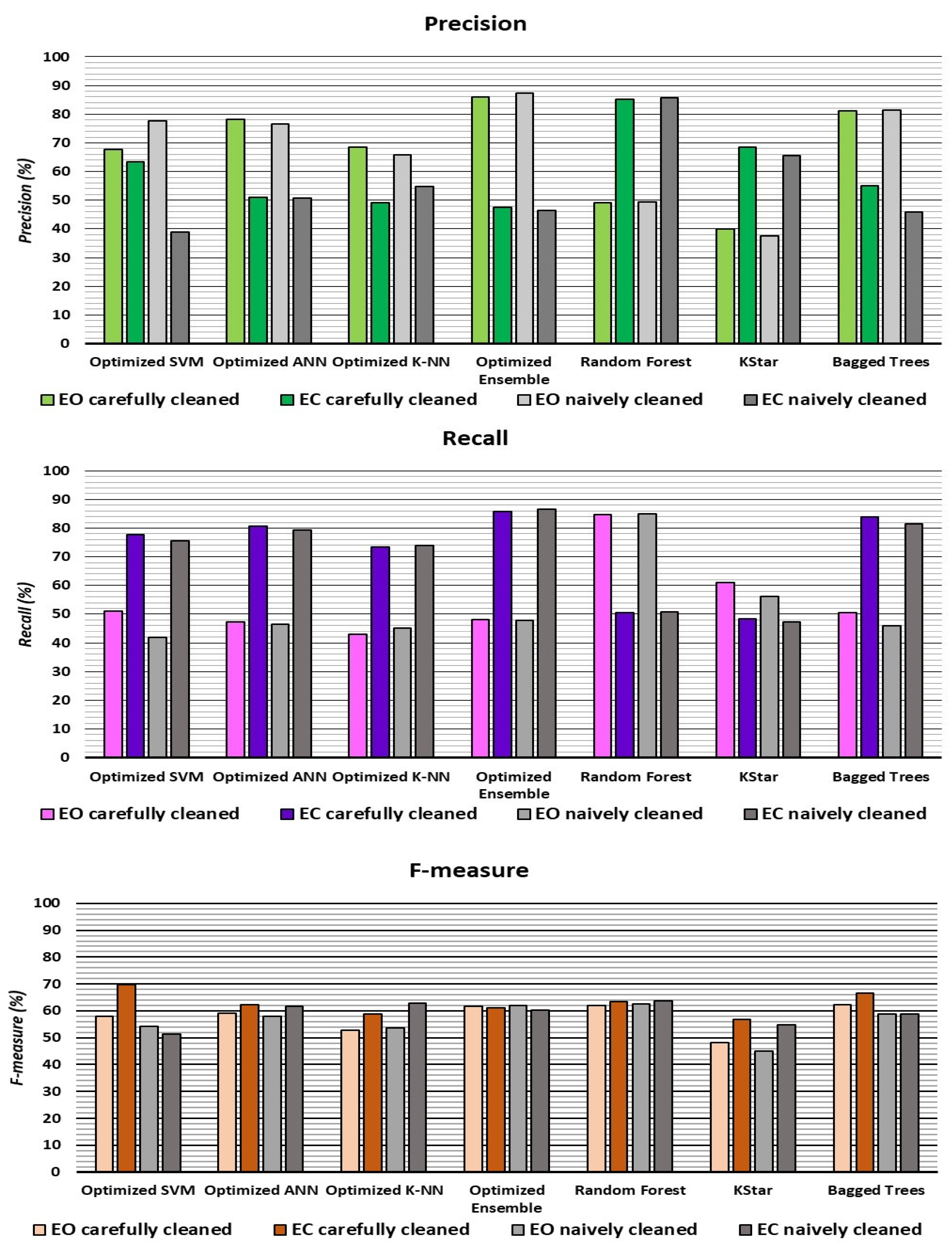
| Optimized SVM | 64.9 | 67.6 | 63.3 | 51.0 | 77.6 | 58.1 | 69.7 | 52.9 | 77.6 | 38.9 | 41.8 | 75.5 | 54.3 | 51.3 |
| Optimized ANN | 60.8 | 78.3 | 50.9 | 47.4 | 80.6 | 59.1 | 62.4 | 59.9 | 76.5 | 50.6 | 46.6 | 79.2 | 57.9 | 61.7 |
| Optimized K-NN | 56 | 68.5 | 49.0 | 43.1 | 73.3 | 52.9 | 58.7 | 58.7 | 65.9 | 54.7 | 45.1 | 74.0 | 53.6 | 62.9 |
| Random Forest | 62.8 | 49.1 | 85.3 | 84.6 | 50.6 | 62.1 | 63.5 | 63.1 | 49.4 | 85.7 | 85.0 | 50.8 | 62.5 | 63.8 |
| KStar | 52.8 | 39.9 | 68.6 | 60.9 | 48.3 | 48.2 | 56.7 | 50.6 | 37.5 | 65.6 | 56.1 | 47.2 | 44.9 | 54.9 |
| Bagged Trees | 64.5 | 81.1 | 55.1 | 50.5 | 83.8 | 62.2 | 66.5 | 58.8 | 81.5 | 46.0 | 46.0 | 81.5 | 58.8 | 58.8 |
| TCN | 60.6 | 59.7 | 61.7 | 64.6 | 56.6 | 62.1 | 59.0 | 71.4 | 86.4 | 65.1 | 50.9 | 91.9 | 64.1 | 76.2 |
| DNN | 66.8 | 64.2 | 66.9 | 71.3 | 63.1 | 67.6 | 64.9 | 65.1 | 74.8 | 61.4 | 50.1 | 81.1 | 60.0 | 69.9 |

References
- Altaheri, H.; Muhammad, G.; Alsulaiman, M.; Amin, S.U.; Altuwaijri, G.A.; Abdul, W.; Bencherif, M.A.; Faisal, M. Deep learning techniques for classification of electroencephalogram (EEG) motor imagery (MI) signals: A review. Neural Comput. Appl. 2021, 1–42. [Google Scholar] [CrossRef]
- Ahmed, Z.I.; Sinha, N.; Phadikar, S.; Ghaderpour, E. Automated Feature Extraction on AsMap for Emotion Classification Using EEG. Sensors 2022, 22, 2346. [Google Scholar] [CrossRef]
- Alharthi, M.K.; Moria, K.M.; Alghazzawi, D.M.; Tayeb, H.O. Epileptic Disorder Detection of Seizures Using EEG Signals. Sensors 2022, 22, 6592. [Google Scholar] [CrossRef] [PubMed]
- Abiri, R.; Borhani, S.; Sellers, E.W.; Jiang, Y.; Zhao, X. A comprehensive review of EEG-based brain–computer interface paradigms. J. Neural Eng. 2019, 16, 011001. [Google Scholar] [CrossRef] [PubMed]
- Saha, S.; Mamun, K.A.; Ahmed, K.; Mostafa, R.; Naik, G.R.; Darvishi, S.; Khandoker, A.H.; Baumert, M. Progress in Brain Computer Interface: Challenges and Opportunities. Front. Syst. Neurosci. 2021, 15, 578875. [Google Scholar] [CrossRef] [PubMed]
- Heunis, T.-M.; Aldrich, C.; de Vries, P.J. Recent Advances in Resting-State Electroencephalography Biomarkers for Autism Spectrum Disorder—A Review of Methodological and Clinical Challenges. Pediatr. Neurol. 2016, 61, 28–37. [Google Scholar] [CrossRef]
- Safayari, A.; Bolhasani, H. Depression diagnosis by deep learning using EEG signals: A systematic review. Med. Nov. Technol. Devices 2021, 12, 100102. [Google Scholar] [CrossRef]
- Khosla, A.; Khandnor, P.; Chand, T. A comparative analysis of signal processing and classification methods for different applications based on EEG signals. Biocybern. Biomed. Eng. 2020, 40, 649–690. [Google Scholar] [CrossRef]
- Hartoyo, A.; Cadusch, P.J.; Liley, D.T.J.; Hicks, D.G. Inferring a simple mechanism for alpha-blocking by fitting a neural population model to EEG spectra. PLoS Comput. Biol. 2020, 16, e1007662. [Google Scholar] [CrossRef]
- Barry, R.J.; Clarke, A.R.; Johnstone, S.J.; Magee, C.A.; Rushby, J.A. EEG differences between eyes-closed and eyes-open resting conditions. Clin. Neurophysiol. 2007, 118, 2765–2773. [Google Scholar] [CrossRef]
- Jackson, A.F.; Bolger, D.J. The neurophysiological bases of EEG and EEG measurement: A review for the rest of us. Psychophysiology 2014, 51, 1061–1071. [Google Scholar] [CrossRef] [PubMed]
- Cohen, M.X. Analyzing Neural Time Series Data: Theory and Practice; MIT Press: Cambridge, MA, USA, 2014. [Google Scholar]
- Halgren, M.; Fabó, D.; Ulbert, I.; Madsen, J.R.; Erőss, L.; Doyle, W.K.; Devinsky, O.; Schomer, D.; Cash, S.S.; Halgren, E. Superficial Slow Rhythms Integrate Cortical Processing in Humans. Sci. Rep. 2018, 8, 2055. [Google Scholar] [CrossRef] [PubMed] [Green Version]
- Halgren, M.; Ulbert, I.; Bastuji, H.; Fabó, D.; Erőss, L.; Rey, M.; Devinsky, O.; Doyle, W.K.; Mak-McCully, R.; Halgren, E.; et al. The generation and propagation of the human alpha rhythm. Proc. Natl. Acad. Sci. USA 2019, 116, 23772–23782. [Google Scholar] [CrossRef] [PubMed]
- Murta, T.; Leite, M.; Carmichael, D.W.; Figueiredo, P.; Lemieux, L. Electrophysiological correlates of the BOLD signal for EEG-informed fMRI. Hum. Brain Mapp. 2014, 36, 391–414. [Google Scholar] [CrossRef] [Green Version]
- Khosla, A.; Khandnor, P.; Chand, T. A novel method for EEG based automated eyes state classification using recurrence plots and machine learning approach. Concurr. Comput. Pract. Exp. 2022, 34, e6912. [Google Scholar] [CrossRef]
- Ketu, S.; Mishra, P.K. Hybrid classification model for eye state detection using electroencephalogram signals. Cogn. Neurodyn. 2021, 16, 73–90. [Google Scholar] [CrossRef]
- Ahmadi, N.; Nilashi, M.; Minaei-Bidgoli, B.; Farooque, M.; Samad, S.; Aljehane, N.O.; Zogaan, W.A.; Ahmadi, H. Eye State Identification Utilizing EEG Signals: A Combined Method Using Self-Organizing Map and Deep Belief Network. Sci. Program. 2022, 2022, 4439189. [Google Scholar] [CrossRef]
- Bird, J.J.; Faria, D.R.; Manso, L.J.; Ayrosa, P.P.; Ekart, A. A study on CNN image classification of EEG signals represented in 2D and 3D. J. Neural Eng. 2021, 18, 026005. [Google Scholar] [CrossRef]
- Ma, P.; Gao, Q. EEG Signal and Feature Interaction Modeling-Based Eye Behavior Prediction Research. Comput. Math. Methods Med. 2020, 2020, 2801015. [Google Scholar] [CrossRef]
- Piatek, Ł.; Fiedler, P.; Haueisen, J. Eye state classification from electroencephalography recordings using machine learning algorithms. Digit. Med. 2018, 4, 84–95. [Google Scholar] [CrossRef]
- Bommisetty, S.H.; Nalam, S.S.A.; Vardhan, J.S.; Ashok, S. Detection of Eye State using Brain Signal Classification with EBPTA and KNN Algorithm. In Proceedings of the 2021 Innovations in Power and Advanced Computing Technologies (i-PACT), Kuala Lumpur, Malaysia, 27–29 November 2021; pp. 1–6. [Google Scholar] [CrossRef]
- Mohamed, A.M.A.; Uçan, O.N.; Bayat, O.; Duru, A.D. Classification of Resting-State Status Based on Sample Entropy and Power Spectrum of Electroencephalography (EEG). Appl. Bionics Biomech. 2020, 2020, 8853238. [Google Scholar] [CrossRef] [PubMed]
- Han, C.-H.; Choi, G.-Y.; Hwang, H.-J. Deep Convolutional Neural Network Based Eye States Classification Using Ear-EEG. Expert Syst. Appl. 2021, 192, 116443. [Google Scholar] [CrossRef]
- Antoniou, E.; Bozios, P.; Christou, V.; Tzimourta, K.; Kalafatakis, K.; Tsipouras, M.G.; Giannakeas, N.; Tzallas, A. EEG-Based Eye Movement Recognition Using Brain–Computer Interface and Random Forests. Sensors 2021, 21, 2339. [Google Scholar] [CrossRef] [PubMed]
- Cohen, W.W. Fast effective rule induction. In Proceedings of the Twelfth International Conference on Machine Learning, Tahoe City, CA, USA, 9–12 July 1995; pp. 115–123. [Google Scholar]
- Frank, E.; Witten, I.H. Generating accurate rule sets without global optimization. In Proceedings of the ICML’98: Proceedings of the Fifteenth International Conference on Machine Learning, Madison, WI, USA, 24–27 July 1998. [Google Scholar]
- Landwehr, N.; Hall, M.; Frank, E. Logistic Model Trees. Mach. Learn. 2005, 59, 161–205. [Google Scholar] [CrossRef] [Green Version]
- Quinlan, R.J. C4.5: Programs for Machine Learning, 1st ed.; Morgan Kaufmann: Burlington, MA, USA, 1992. [Google Scholar]
- Breiman, L. Random Forests. Mach. Learn. 2001, 45, 5–32. [Google Scholar] [CrossRef] [Green Version]
- Bai, S.; Zico Kolter, J.; Vladlen, K. An Empirical Evaluation of Generic Convolutional and Recurrent Networks for Sequence Modeling. arXiv 2018, arXiv:1803.01271. [Google Scholar]
- Aha, D.W.; Kibler, D.; Albert, M.K.; Quinian, J.R. Instance-based learning algorithms. Mach. Learn. 1991, 6, 37–66. [Google Scholar] [CrossRef] [Green Version]
- Cleary, J.G.; Trigg, L.E. K*: An Instance-based Learner Using an Entropic Distance Measure. In Proceedings of the Twelfth International Conference on Machine Learning, Tahoe City, CA, USA, 9–12 July 1995; pp. 108–114. [Google Scholar]
- Statistics and Machine Learning Toolbox; The MathWorks Inc.: Natick, MA, USA, 2022.
- Le Cessie, S.; Van Houwelingen, J.C. Ridge Estimators in Logistic Regression. Appl. Stat. 1992, 41, 191–201. [Google Scholar] [CrossRef]
- Hall, M.; Frank, E.; Holmes, G.; Pfahringer, B.; Reutemann, P.; Witten, I.H. The WEKA data mining software: An update. ACM SIGKDD Explor. Newsl. 2009, 11, 10–18. [Google Scholar] [CrossRef]
- MATLAB; The MathWorks Inc.: Natick, MA, USA, 2022.
- Powers, D.; Ailab. Evaluation: From precision, recall and F-measure to ROC, informedness, markedness & correlation. J. Mach. Learn. Technol. 2011, 2, 2229–3981. [Google Scholar] [CrossRef]


| Name | Number of Data Instances | Subjects Contributing to the Data | Number of Features | Class Distribution | |
|---|---|---|---|---|---|
| EO | EC | ||||
| CP50 | 9481 | All 50 | 96 | 4711 | 4770 |
| SP50 | 6603 | All 50 | 96 | 3031 | 3572 |
| CP40-M, SP40-M | 5328 * | Subjects 11–50, 40 in total | 96 | 2216 | 3112 |
| CP10 | 1884 | Subjects 1–10, 10 in total | 96 | 940 | 944 |
| SP10, CP10-M | 1275 * | Subjects 1–10, 10 in total | 96 | 460 | 815 |
| CPR40-TR, SPR-40TR | 5328 * | Various, randomly selected | 96 | 2216 | 3112 |
| CPR10-TE, SPR10-TE | 1275 * | Various, randomly selected | 96 | 460 | 815 |
| Models | Accuracy (%) | Precision (%) | Recall (%) | F-Measure (%) | ||||||||||
|---|---|---|---|---|---|---|---|---|---|---|---|---|---|---|
| EO | EC | EO | EC | EO | EC | |||||||||
| CP50 | SP50 | CP50 | SP50 | CP50 | SP50 | CP50 | SP50 | CP50 | SP50 | CP50 | SP50 | CP50 | SP50 | |
| Optimized Ensemble | 98.3 | 99.0 | 98.4 | 94.9 | 98.2 | 98.5 | 98.1 | 98.2 | 98.4 | 95.8 | 98.2 | 96.5 | 98.3 | 97.1 |
| Optimized SVM | 97.4 | 96.9 | 98.0 | 96.4 | 96.8 | 97.3 | 96.8 | 96.9 | 98.0 | 97.0 | 97.4 | 96.6 | 97.4 | 97.1 |
| Optimized ANN | 97.1 | 97.1 | 95.6 | 95.0 | 98.6 | 98.9 | 98.6 | 98.6 | 95.7 | 95.9 | 97.1 | 96.8 | 97.1 | 97.4 |
| Random Forest | 96.9 | 97.0 | 97.6 | 96.7 | 96.2 | 97.4 | 96.1 | 97.8 | 97.6 | 96.0 | 96.8 | 97.2 | 96.9 | 96.7 |
| Optimized K-NN | 96.8 | 96.1 | 95.1 | 93.5 | 98.4 | 98.3 | 98.3 | 97.9 | 95.3 | 94.7 | 96.7 | 95.6 | 96.8 | 96.5 |
| KStar | 95.8 | 95.3 | 97.9 | 94.1 | 93.9 | 96.9 | 93.5 | 97.5 | 98 | 92.8 | 95.7 | 95.8 | 95.9 | 94.8 |
| Bagged Trees | 95 | 96.9 | 93.2 | 94.9 | 96.7 | 98.5 | 96.5 | 98.2 | 93.6 | 95.8 | 94.8 | 96.5 | 95.1 | 97.1 |
| LMT | 92.6 | 93.6 | 95.4 | 92.0 | 90.1 | 95.7 | 89.4 | 96.6 | 95.7 | 90.1 | 92.3 | 94.2 | 92.8 | 92.8 |
| PART | 90.5 | 90.9 | 92.9 | 90.2 | 88.4 | 92.0 | 87.5 | 93.5 | 93.4 | 88.0 | 90.2 | 91.8 | 90.8 | 89.9 |
| J48 | 88.4 | 88.4 | 90.7 | 86.4 | 86.4 | 90.7 | 85.5 | 91.3 | 91.3 | 85.5 | 88 | 88.8 | 88.8 | 88.0 |
| DNN | 86.8 | 86.3 | 90.0 | 91.2 | 84.1 | 82.8 | 79.7 | 78.4 | 92.1 | 91.1 | 84.5 | 84.3 | 87.9 | 86.8 |
| TCN | 84.7 | 83.2 | 89.6 | 88.0 | 81.0 | 79.4 | 78.5 | 76.5 | 91.0 | 89.7 | 83.7 | 81.8 | 85.7 | 84.2 |
| JRip | 85.9 | 87.5 | 87.4 | 87.2 | 84.6 | 87.9 | 83.8 | 90.1 | 88.1 | 84.4 | 85.5 | 86.6 | 86.3 | 88.1 |
| Logistic Regression | 79.4 | 75.9 | 77.4 | 65.4 | 81.6 | 84.9 | 79.9 | 78.5 | 76.2 | 74.3 | 79.9 | 71.4 | 78.8 | 79.2 |
| Study | Subjects (# of Samples) | EEG | Preprocessing | Features Extracted | Best Classifier | Accuracy | Validation | Final Purpose |
|---|---|---|---|---|---|---|---|---|
| [14] | 9 (257) | 16 | The data was preprocessed by filtering (1–40 Hz) and removing epochs exceeding ±100 μV of amplitude | FFT, all available frequency bins used as features (total number not stated). | SVM | 97% | 10-fold CV | The study aimed to identify the brain’s resting status using short-length EEG epochs using both linear and nonlinear features derived from EEG. Aimed at general-purpose applications. * |
| [15] | 10 (112,128) | 32 | Bandpass filtering in the delta, theta, alpha and beta bands. | Delta, theta, alpha and beta band energies (128 features total). | Random Forest | 85.39% | 10-fold CV | This method exploits high spatial information acquired from the Emotiv EPOC Flex wearable EEG recording device and examines successfully the potential of this device to be used for BCI wheelchair technology. Aimed at targeted or person-specific final applications. * |
| [23] | 30 (1800) | 33 | EEG data was first re-referenced to average, then bandpass-filtered between 1 and 50 Hz | Features were extracted based on the FFT in 6 (delta, theta, alpha, beta, gamma and all) different frequency bands, per 6 electrodes in 4 ROIs and 30 trials for each condition (8.640 features total). | CNN | 96.92% | 10-fold CV | Developing a more practical and reliable ear-EEG based application related to eye state classification. Aimed at general-purpose final applications. * |
| 90.81% | Test-retest | |||||||
| [16] | 27 (829,494) | 19 | “Clean” sections of data, without artifacts, were chosen by an expert. | Single electrode data points (19 features) | K-NN (k = 1) | 99.8% | hold-out (66%/34% split) | Predicting eye states using EEG recordings in a real-time system, interpreting classification rules for gaining insight into EEG data. Aimed at general-purpose final applications. * |
| 10 data points of an EEG recording (190 features) | Random Forest | 96.6% | hold-out (66%/34% split) | |||||
| 27 (82,836) | “Clean” sections of data, without artifacts, were chosen by an expert. The data was filtered in the 1–40 Hz range and a notch filter eliminating line noise was applied. | Single electrode data points (19 features) | K-NN (k = 1) | 99.4% | hold-out (66%/34% split) | |||
| 10 data points of an EEG recording (190 features) | Random Forest | 96.5% | hold-out (66%/34% split) | |||||
| [17] | 109 (3270) | 64 | EEG data was preprocessed by applying low pass Butterworth filtering with the cut off frequency of 40 Hz | Six RQA (recurrence quantification analysis)-based measures (recurrence rate, determinism, entropy, laminarity, trapping time, and longest vertical line) had been extracted from 64 EEG channels based on a genetic algorithm (384 features total). | Logistic Regression | 97.27% | 10-fold CV | Automated classification of EEG signals into eyes-open and eyes-close states. The development of the practical applications for performing daily life tasks. Aimed at general-purpose final applications. |
| [18] | 1 (14,980) | Not stated. | No preprocessing. | The features (14 features) of EEG data were extracted based on the wavelet transform (Final number of features not stated). | Deep factorization machine model (FM: +LSTM | 93% | 10-fold CV | The diagnosis of fatigue by detecting eye openness status. Aimed at general-purpose final applications. |
| [19] | 1 (14,980) | 14 | Clustering into dissimilar groups by Self-organizing map (SOM). Classification performed within each cluster. | No feature extraction, raw signal used. | Deep Belief Network (DBN) | 95.2% | 10-fold CV | The study investigates eye state identification using EEG signals. Aimed at general-purpose final applications. * |
| [20] | 1 (15,181) | 14 | Dataset cleaned by removing the missing values as well as outliers based on the “Isolation Forest’’ technique | No feature extraction, raw signal used. | Hypertuned SVM | 98.5% | 10-fold CV (70/30 split) | Medical appliances capable of classifying various bodily states, drug effects etc. Aimed at general-purpose final applications. |
| [21] | 10 (Not stated) | 64 | No preprocessing. | Mean value of each sliding window, asymmetry and peakedness, maximum and minimum, complex logarithm of sample covariance matrix, 10 most energetic FFT components, all windows also inherit features of previous windows that are different from the current ones (Variable number of total features for each window.) | CNN | 97.96% | 10-fold CV | The approach is dynamically applicable to BCI devices of higher resolution and problems other than the frontal lobe activity classification. Aimed at targeted or person-specific final applications. * |
| 83.3% | “Leave-one-out” CV | |||||||
| [22] | 1 (14,980) | 14 | First, the Independent Component Analysis (ICA) algorithm is employed to remove the artifacts from EEG data, then the data is Fast Fourier Transformed. | Fast Fourier Transform, time analysis, time-frequency analysis using the STFT, and time-frequency-space analysis extracted characteristics of data were chosen as features based on the results of Principle Component Analysis (14 features). | EBPTA | 98.94% | 10-fold CV | The eye status categorization from brain activity signals and its application to real time applications. Aimed at general-purpose final applications. * |
| This paper | 50 (6603) | 24 | Visual inspection of the dataset to assess its usability, filtering (1–50 Hz), epoching of the data into 2 s long epochs, removal of any epochs where the voltage observed exceeds ±100 μV. | Welch FFT acquired frequency bin powers encompassing the ranges of 4–7 Hz, 8–13 Hz, 13–30 Hz and 30–50 Hz were averaged to obtain the powers of the Θ, α, β and ɣ frequency bands. This was done for the data obtained from each of the 24 electrodes that comprised the EEG datasets, resulting in 96 features and 1 binary nominal target variable. | Ensemble Classifier | 99% | 10-fold CV | Final purpose is the evaluation of the effects of preprocessing and validation methods on classifier accuracy. |
| 50 (6603) | Random Forest | 63.1% | Hold-out (40 subjects/10 subjects) | |||||
| 50 (9481) | Visual inspection and rejection of obvious electrode detachment/malfunction and other similar types of artifacts, filtering (1–50Hz), independent component analysis (ICA) decomposition, rejection of artifact independent components, channel automatic rejection by spectrum, ±3 SD outlier channels removed, visual inspection and rejection of any remaining artifact data, re-referencing to average, blind source separation (BSS) correction of muscle artifacts, interpolation of missing channels, epoching of the data into 2 s long epochs. | Ensemble Classifier | 98.3% | 10-fold CV | ||||
| 50 (6603) | SVM | 64.9% | hold-out (40 subjects/10 subjects) |
Disclaimer/Publisher’s Note: The statements, opinions and data contained in all publications are solely those of the individual author(s) and contributor(s) and not of MDPI and/or the editor(s). MDPI and/or the editor(s) disclaim responsibility for any injury to people or property resulting from any ideas, methods, instructions or products referred to in the content. |
© 2022 by the authors. Licensee MDPI, Basel, Switzerland. This article is an open access article distributed under the terms and conditions of the Creative Commons Attribution (CC BY) license (https://creativecommons.org/licenses/by/4.0/).
Share and Cite
Mattiev, J.; Sajovic, J.; Drevenšek, G.; Rogelj, P. Assessment of Model Accuracy in Eyes Open and Closed EEG Data: Effect of Data Pre-Processing and Validation Methods. Bioengineering 2023, 10, 42. https://doi.org/10.3390/bioengineering10010042
Mattiev J, Sajovic J, Drevenšek G, Rogelj P. Assessment of Model Accuracy in Eyes Open and Closed EEG Data: Effect of Data Pre-Processing and Validation Methods. Bioengineering. 2023; 10(1):42. https://doi.org/10.3390/bioengineering10010042
Chicago/Turabian StyleMattiev, Jamolbek, Jakob Sajovic, Gorazd Drevenšek, and Peter Rogelj. 2023. "Assessment of Model Accuracy in Eyes Open and Closed EEG Data: Effect of Data Pre-Processing and Validation Methods" Bioengineering 10, no. 1: 42. https://doi.org/10.3390/bioengineering10010042