Integration of Unmanned Aerial Vehicle Imagery with Landsat Imagery for Better Watershed Scale ET Prediction

Abstract

Evapotranspiration (ET) is a critical component of the water cycle, and an accurate prediction of ET is essential for water resource management, irrigation scheduling, and agricultural productivity. Traditionally, ET has been estimated using satellite-based remote sensing, which provides synoptic coverage but can be limited in spatial resolution and accuracy. Unmanned aerial vehicles (UAVs) offer improved ET prediction by providing high-resolution imagery of the Earth’s surface but are limited to a small area. Therefore, UAV and satellite images provide complementary data, but the integration of these two data for ET prediction has received limited attention. This paper presents a method that integrates UAV and satellite imagery for improved ET prediction and applies it to five crops (corn, rye grass, wheat, and alfalfa) from agricultural fields in the Walla Walla of eastern Washington State. We collected UAV and satellite data for five crops and used the combination of remote sensing models and statistical techniques to estimate ET. We show that UAV-based ET can be integrated with the Landsat-based ET with the application of integration factors. Our result shows that the Root Mean Square Error (RMSE) of daily ET for corn (Zea mays), rye grass (Lolium perenne), wheat (Triticum aestivum), peas (Pisum sativum), and alfalfa (Medicago sativa) can be improved by the application of the integration factor to the Landsat based ET in the range of (35.75–65.52%). We also explore the variability and effect of partial cloud on UAV-based ET estimation. Our findings have implications for the use of UAVs in water resource management and highlight the importance of considering multiple sources of data in ET prediction.

1. Introduction

The allocation of water resources at the watershed scale is being challenged globally by decreasing supplies and increasing demands [1,2,3,4]. Efficient water management is critical for balancing the needs of sustainable irrigated agriculture, ecosystem services, and water for future development. Effective resource management requires reliable information on water availability and demands, especially for irrigated crops that account for nearly 80% of consumptive use in agricultural basins [5,6,7]. In these basins, understanding water balances requires accurate estimation of consumptive use at the watershed scale. However, measurement and prediction of evapotranspiration (ET) at a regional or watershed scale is challenging due to its spatial and temporal complexity.

Remote sensing images have provided a promising source of data for mapping ET over large areas in cost-effective ways [8,9,10,11,12] and have been increasingly used for mapping ET [13,14,15]. One advantage of remote sensing images is that they do not require knowledge of the crop growth stage, as they establish a direct link between surface radiances and energy balance components. The critical surface and atmospheric variables necessary for simulating surface fluxes and ET, such as land surface temperature, vegetation indices, and atmospheric temperature, can be retrieved from visible, near infrared, and thermal infrared bands of sensors. However, the resolution of ET products derived from satellite images, such as those from Moderate Resolution Imaging Spectroradiometer (MODIS), may not be sufficient to capture the spatial variability of ET due to their lower resolution (~500 m ground pixel resolution). Other open-source satellite imagery, such as Landsat and Sentinel, have higher resolution (Landsat visible, NIR, SWIR—30 m, thermal—100 m; Sentinel: 10 m) but have long revisit cycles (e.g., 16 days for Landsat 8). As a result, we may miss important crop growth stages and potentially underestimate seasonal consumptive use. This gap can be reduced with the availability of Landsat 9 having anoverpass of 8 days with Landsat 8. Nevertheless, satellite images can also be obscured by cloud cover, therefore, we may still not have a single image even in a month. Additionally, there is a tradeoff between scanning swath and pixel size, therefore, none of the existing satellite sensors can provide images with both high temporal and spatial resolution [16,17]. There is a high demand for spatially explicit ET information at a higher spatial resolution, for example in precision agriculture [18,19]. With the possibility of frequent flights and higher spatial resolution, the Unmanned Aerial Vehicle (UAV) stands out as a promising technology for filling this gap of satellite imagery.

UAVs equipped with multispectral and thermal sensors have become powerful tools for mapping ET from agricultural fields as they can produce flights on demand and provide images with higher resolution. The ground pixel resolutions for these systems are in the order of 0.02–0.10 m for multispectral and 0.4–1.0 m for thermal sensors [20,21]. The development of software, for example, Pix4D and Agisoft Metashape, for post-processing has helped in the wide application of UAV technology including assessing olive tree crown parameters, estimating energy balance components over orchards, corn field testing, and mapping surface and direct-root-zone water use [19,22,23,24,25]. However, UAV capabilities are limited by their ability to cover only small areas due to their limited flying time because of the batteries’ endurance and low consumer-grade cameras [26]. Most consumer-grade UAVs are not equipped with a thermal sensor which is indispensable for ET estimation using a surface energy balance algorithm [27,28]. Even so, they can still collect a large block of images with a centimeter-scale spatial resolution and can be useful for mapping important growth stage of crops.

Therefore, UAV and satellite remote sensing data complement each other. The advantages of satellite remote sensing data appear to compensate for the disadvantage of the UAV, and vice versa with an opportunity for synergies of these two sources. There are some recent studies that have applied the synergy of these two remote sensing information sources. For example, Backes and Teferle [21] used UAV imagery with satellite imagery for mapping a high accuracy digital elevation model, and Gray, et al. [29] used UAV imagery in combination with satellite imagery to assess estuarine environments. Similarly, Bhatnagar, et al. [30] used a nested UAV-satellite approach to monitor the ecological wetlands. Although there are recent studies that attempted to combine Landsat and UAV imagery for better ET estimation [20], they did not examine how Landsat ET compares with UAV ET estimations across different crops and whether correction is needed for watershed-scale prediction. Since UAV-based mapping costs sizeable investment for mapping ET, we need to examine whether UAV-based mapping warrants the further investment in it.

While UAV-based mapping is good for precision agriculture providing the spatially explicit information, watershed-scale application needs the information of whether there is a difference in the ET mapped using the two sensors at spatial resolution of satellite imagery. Before investing time and resource into developing an algorithm for joint analysis of data from these two sources, we need information about how these two sources perform in terms of mapping ET. Similarly, a lot of literature asserts that UAV’s flexibility to fly on cloudy days and the possibility of capturing higher variability of ET is the added advantage over similar other remote sensing techniques [31,32]. The effects of the cloud-based illumination impact on the ET mapping from agricultural fields are not yet well understood. UAV can be flown under the cloud, but the changing weather can affect how the sensor interprets data from the ground. Therefore, for mapping ET and subsequent integration, understating the effect of clouds on UAV-based ET estimation is essential.

The objective of this research is to improve the watershed scale ET estimation using UAV images in conjunction with Landsat images. To achieve this objective, we estimated, compared and developed a method for successful integration of ET over agricultural field using Landsat images with the image collected by Mica Sense Altum sensor mounted on DJI Matrice 210 Quadcopter. The differences in ET across sensors are used for calculation of the integration factor, which is applied for ET estimation at places when and where UAV is not flown. We also assess the effect of cloud on UAV-based ET prediction by comparing ET under partial cloud and cloud free conditions. We specifically address the following questions: (1) Is there a sizeable difference in ET mapped at field scale using UAV-based and satellite-based imagery? (2) Is there a time to be careful for taking UAV based imagery (effect of partial cloud)? (3) Is there a way to integrate these two sources either spatially or temporally using an integration factor? We show that there is a sizeable difference in ET creating a ground for further investment in drone-based imagery acquisition and potential for integration of two sensors for watershed scale prediction by applying a integration factor.

2. Materials and Methods

2.1. Study Area

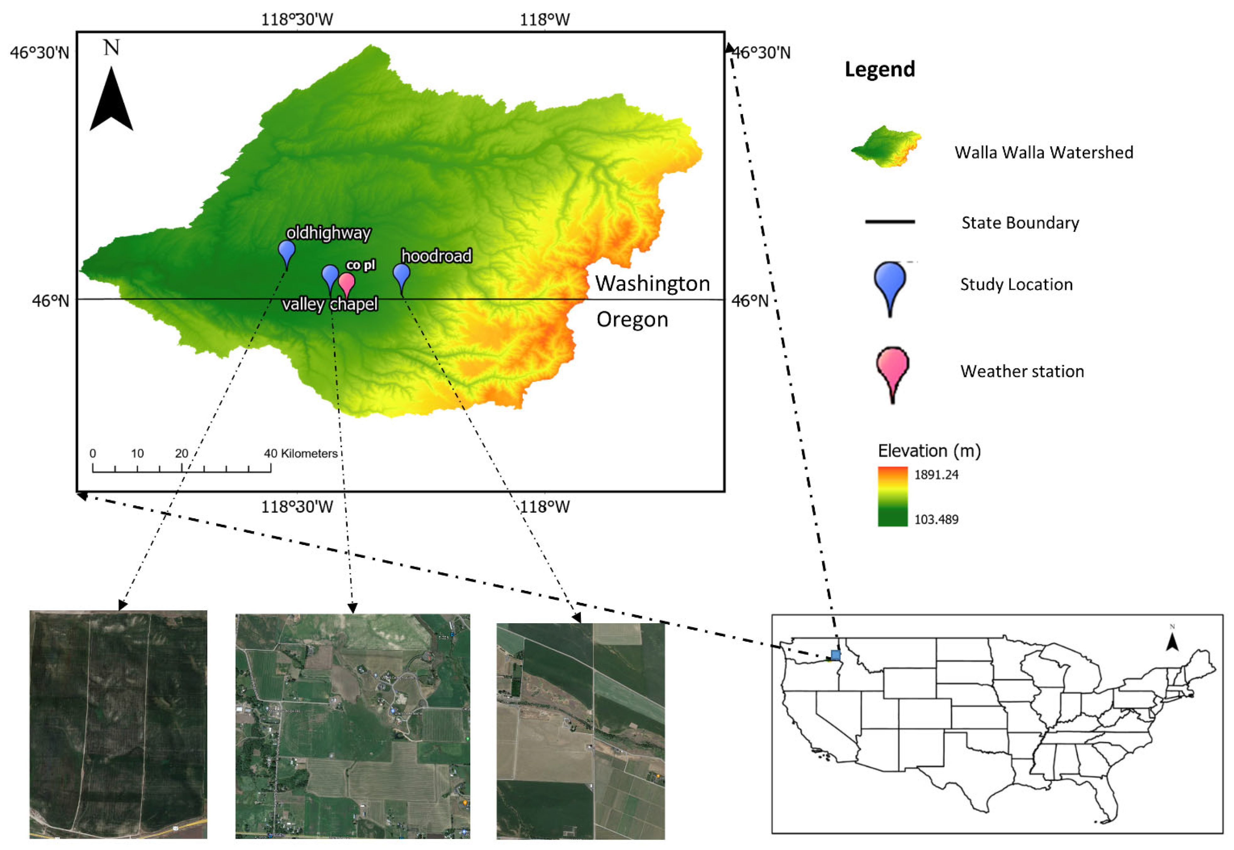
This study was conducted in the Walla Walla River basin, located in the Pacific Northwestern U.S. It is a bi-state watershed in the southeast Washington and northeast Oregon (Figure 1). In Walla Walla, the summers are hot and dry (average July maximum temperature of 34 °C and rainfall of ~10 mm) while the winters are cold and snowy (average December minimum temperature of 0 °C and snowfall of ~68 mm) with variable precipitations in the region ranging from 1143 mm/year in mountainous headwaters to 254 mm/year near its confluence with the Columbia River. The major crops in the region include alfalfa, corn, peas, rye grass, and wheat.

Table 1. Details of the experimental field sites used for mapping UAV imagery with types of crops, irrigation system, acquisition time of UAV images, Landsat overpass, and location. The acquisition time of UAV images and Landsat overpass are reported in 24-h format Pacific Daylight Saving Time (PDT). Sites 1–5 are located in valley Chapel, sites 6 and 7 are located in old highway, and sites 8–10 are located in hood road areas in Walla Walla, WA. Two UAV acquisitions were performed on Site 3 on 20 June 2022.

Crop	Day Month Year	Sites	Time of UAV Acquisition	Time of Landsat Overpass	Location	Irrigation System
Alfalfa	11 July 2021	Site 8	10:07	11:43	Hood Road	Hand Line
	11 May 2022	Site 4	09:47	11:43	Valley Chapel	Center Pivot
	11 May 2022	Site 8	12:15	11:43	Hood Road	Hand Line
	12 May 2022	Site 5	11:18	11:37	Valley Chapel	Center Pivot
	21 June 2022	Site 8	13:10	11:37	Hood Road	Hand Line
Wheat	11 July 2021	Site 10	13:45	11:43	Hood Road	Hand Line
	21 June 2022	Site 6	10:07	11:37	Old Highway	Wheel Line
	21 June 2022	Site 7	10:40	11:37	Old Highway	Wheel Line
Rye grass	11 May 2022	Site 1	10:12	11:43	Valley Chapel	Center Pivot
	11 May 2022	Site 2	10:35	11:43	Valley Chapel	Center Pivot
	12 May 2022	Site 2	12:43	11:37	Valley Chapel	Center Pivot
	21 June 2022	Site 2	12:10	11:37	Valley Chapel	Center Pivot
Peas	11 May 2022	Site 9	13:02	11:43	Hood Road	Center Pivot
	11 May 2022	Site 10	13:30	11:43	Hood Road	Hand Line
	21 June 2022	Site 10	13:42	11:37	Hood Road	Hand Line
Corn	11 July 2021	Site 1	12:25	11:43	Valley Chapel	Center Pivot
	11 July 2021	Site 4	11:37	11:43	Valley Chapel	Center Pivot
	11 July 2021	Site 9	11:07	11:43	Old Highway	Center Pivot
	20 June 2022	Site 3	10:45	11:27	Valley Chapel	Center Pivot

presents the details of experimental field sites along with types of crops, irrigation systems, acquisition time of UAV images, Landsat overpass, and geolocation of each site. A total of 10 sites were used, mainly located in the three regions of Walla Walla that are designated as “old highway”, “valley chapel”, and “hood road” (Figure 1, Table 1). We selected five different types of crops (corn, rye grass, wheat, and alfalfa) with three irrigation types (center pivot, hand line, and wheel line).

2.2. Data

2.2.1. Satellite Imagery

Table 2. Details of Landsat used in this study with their types, path and row ids and selected area cloud cover.

Day Month Year	Landsat Types	PathID	RowID	Cloud Cover (%)
11 July 2021	Landsat 8	44	28	0
11 May 2022	Landsat 8	44	28	5
12 May 2022	Landsat 9	43	28	7.5
21 June 2022	Landsat 8	43	28	3

provides detail information about the satellite images used with their path and row. We used three Landsat 8 and one Landsat 9 images, which were extracted from earth explorer.

2.2.2. UAV Imagery

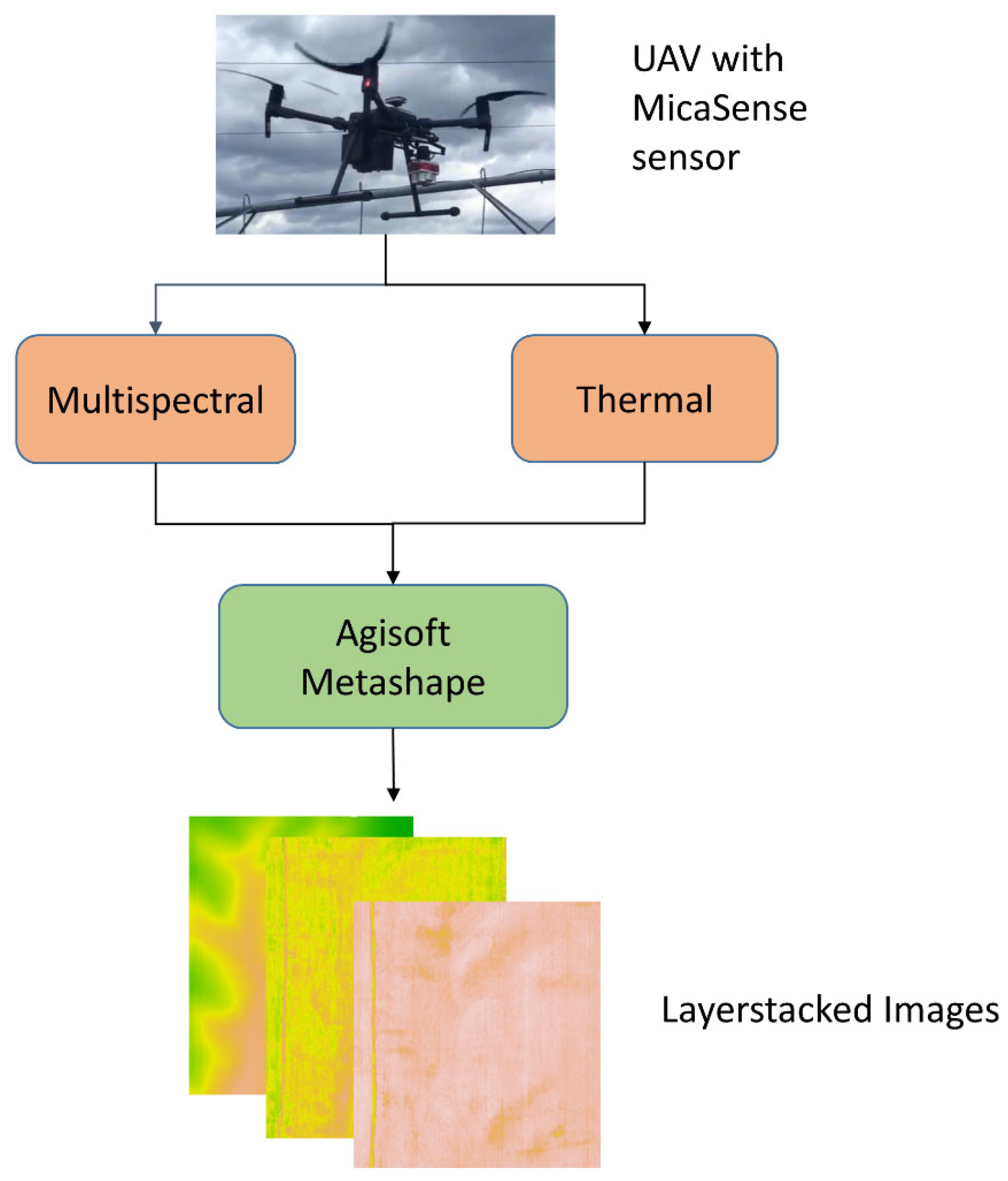
Three field trips were made to Walla Walla covering two growing seasons for five crop fields: alfalfa, corn, peas, rye grass, and wheat. We collected images of these fields, flying UAV (DJI Matrice 210) equipped with a high-resolution multispectral and thermal sensor (MicaSense Altum) on the same days and approximate times as the Landsat passes. However, UAV acquired images of 20 June 2022 were discarded for comparison and integration as the Landsat image on that day was obscured by clouds. The spatial resolution of the UAV-based imagery is variable depending upon flying altitude and the spectral bands. For consistency, the UAV was flown at an altitude of 70 m resulting in a thermal band resolution of ~0.6 m and multispectral band resolution ~0.03 m. Raw images were preprocessed using Agisoft Metashape software Version 1.8.3. The detailed processes are depicted in Figure 2. The images were ortho-rectified and layerstacked to achieve a single TIFF file containing blue, green, red, red-edge, infrared, and thermal bands. A separate TIFF file was created for the DEM at the same resolution as that of the orthomosaic. An orthomosaic image from the Agisoft Metashpae was exported at a 0.6-m thermal band resolution aggregating (taking the average) of the multispectral values by a factor of 20. Further processing was performed in R, a statistical programming language [33]. The orthomosaic image extracted from the Agisoft Metashape did not provide the direct surface reflectance values which were converted to the surface reflectance by dividing each band by 32,768 [34]. Similarly, the orthomosaic thermal data retrieved from Agisoft Metashape was converted to kelvin by dividing the orthomosaic thermal band by 100 as instructed in the user guide [35].

2.2.3. Weather Data

Instantaneous (every 15 min) weather data from the Agweathernet station at College Place Walla Walla were extracted for the days of the UAV flights and satellite overpasses.

Table 3. Average daily weather data (minimum temperature, maximum temperature, average relative humidity, wind speed, precipitation, and solar radiation) on the days of UAV acquisitions used in this study.

Day Month Year	Min Temp (°C)	Max Temp (°C)	Avg RH%	Wind Speed (m/s)	Precipitation (mm)	Solar Radiation (MJ/m2)
11 July 2021	16.6	36.2	35.2	1.9	0	29.7
11 May 2022	1.4	17.8	66.2	1.7	0	28.4
12 May 2022	3.9	17.7	80.0	2.1	9.4	15.2
20 June 2022	12.2	24.8	71.8	1.9	0	26.0
21 June 2022	8.7	28.8	72.4	1.3	0	29.7

provides the summary of weather data for the study period.

2.2.4. Elevation Data

Digital Elevation Model (DEM) data at 30-m resolution was obtained from the USGS National Elevation Dataset. We also used the DEM created at 0.6 m resolution for the UAV based model.

2.2.5. Land Cover Data

Land cover data were extracted from USGS National Land Cover Database 2016 to identify the agricultural land use pixels and pasture land use pixels required for this study.

2.3. Co-Registration of the Images

Table 4. Wavelength across the sensors for multispectral (blue, green, red, and near infrared) and thermal band used in this study. UAV represent the MicaSense Altum sensor and Landsat represent the Operational Landsat Imager.

Band Name	Wavelength (nm)
	UAV	Landsat
Blue	459–491	450–510
Green	546.5–573.5	533–590
Red	661–675	640–670
NIR	813.5–870.5	850–880
Thermal	800–1400	1060–1251

provides the wavelengths of the four spectral bands and thermal band across the UAV (MicaSense Altum), and Landsat (OLI) sensors. Table 4 shows similar wavelengths for all the bands (blue, green, red, near infrared, and thermal) in the case of both UAV and Landsat sensors, allowing us to combine the data. The pixels of the UAV images may not be exactly lined up with the satellite imagery. To line up the UAV-based pixel imagery with Landsat, co-registration of the images is required. Thus, the 30-m resolution Landsat images were cropped by the field extent and were downscaled (i.e., upsampled) to 0.6-m resolution using a factor of 50. Finally, orthomosaic UAV images at ~0.6-m resolution were resampled to the resolution and extent of downscaled Landsat images.

2.4. METRIC Model

We applied widely used evapoTranspiration mapping at high Resolution with Internalized Calibration (METRIC) model to quantify ET [36,37,38]. METRIC is an image processing tool for mapping ET as a residual of the energy balance at the Earth’s surface. In this model, instantaneous ET is computed by dividing the difference of the available energy ($R_n$ − G) and sensible heat flux (H) by latent heat of vaporization (λ) as below (Equation (1)).

$$ET=\frac{R_n-G-H}{\mathsf{\lambda }}$$

(1)

where $R_n$ is the net radiation (W·m⁻²), and G is the soil heat flux (W·m⁻²).

METRIC requires identification of two anchor pixels (hot and cold) to establish a relation between land surface temperature and the difference between radiant temperature by fixing the boundary condition for internal calibration. Typically, cold conditions correspond to well irrigated fields and hot conditions correspond to bare agricultural fields. These two pixels are used as boundary conditions to find temperature gradients (dT) at each pixel. Then, dT is used to determine the coefficients (i.e., slope and intercept) of a linear relationship between dT and land surface temperature (Ts) across the entire image as below (Equation (2)).

$$dT=aTs+b$$

(2)

where a and b are empirical constants and are determined using extreme end conditions, i.e., with cold pixel (representing maximum Latent Energy) and hot pixel (representing zero Latent Energy). For more details, we refer to Allen, et al. [39].

The process of mapping actual ET is almost the same for both Landsat and UAV images with the only different equation being the one used for albedo calculations. Since detailed processes have been explained in many literatures, only the difference in albedo calculations is explained here. UAV data obtained with a MicaSense sensor lacks the shortwave band necessary for surface albedo estimation, thus we employed Equations (3) and (4) to estimate the surface albedo ($\propto$) using narrow band data as suggested by Brest and Goward [40]. The surface albedo for satellite images is expressed as (Equation (3)),

$${\propto =\sum (w_b\times ⍴}_b)$$

(3)

where $w_b$ is the weight of each band in the Landsat 8 spectral range, ${\mathrm{⍴}}_b$ is the reflectance of each band. Similarly, surface albedo for UAV images is expressed as (Equation (4)),

$$\begin{gathered} \propto =0.526\left(VIS\right)+0.362\left(NIR\right)+0.112\left[0.5\left(NIR\right)\right],NDVI\ge 0.25 \\ \propto =0.526\left(VIS\right)+0.474\left(NIR\right),NDVI<0.25 \end{gathered}$$

(4)

where, VIS is the reflectance corresponding to the visible bands, NIR is the reflectance of the Near Infrared band of the UAV, and NDVI is the Normalized Difference Vegetation Index computed as (Equation (5)).

$$NDVI=\frac{NIR-R}{NIR+R}$$

(5)

where, NIR is the Near Infrared band and R is the Red band.

Implementation of the METRIC Model

The METRIC model for this research was developed using the “Water” package available in R [41], a statistical programming language [33]. The Water package was initially developed for estimating the ET using Landsat 7 imagery and was modified by the developer to estimate Landsat-8 ET. For our work we used this package to estimate the ET using Landsat 8 and Landsat 9 imagery. The original package was then modified for ET calculation using UAV imagery. Since ET estimation using METRIC model is reliant on identification of anchor pixels within an image, we captured the images of agricultural fields including boundaries like road and bare lands in each flight in order to include anchor pixels within a layerstacked image. The anchor pixels were chosen using the Water package’s implementation of detecting hot and cold pixels. The package values were then manually checked for their locations in expected well-watered plant land and barren ground for cold and hot pixels, respectively, using visual inspection as suggested in Molaei, et al. [42].

2.5. Comparison of ET

The comparisons between Landsat estimated ET and UAV estimated ET were performed for each day of satellite overpass to determine the similarity or dissimilarity in daily ET estimation between the sensors. First, ET was estimated separately for both UAV and Landsat imagery for the same field on the same day using METRIC. Then, Landsat estimated ET was cropped by the extent of the field, using the UAV imagery for comparison purposes. Similarly, ET for UAV imagery was estimated at a thermal resolution of 0.6 m, which was upscaled to a Landsat resolution of 30 m by aggregating (taking the mean value) the UAV ET with factor of 50. The pixel-by-pixel comparisons between the ET estimated using two sensors were performed at the Landsat resolution of 30 m. The variations in the patterns were tested by plotting the two raster images side by side using the same color scale for five samples (one for each crop). The statistical comparison between the ET were tested using the five statistical measures; the coefficient of determination (R²), Root Mean Square Error (RMSE), Mean Absolute Error (MAE), bias, and median.

2.6. Partial Cloud Effect on UAV-ET

To understand the potential impact of partial cloud on UAV-based ET prediction, we estimated and compared the ET prediction under partial cloud cover and clear sky conditions over site 3 on 20 June 2022. UAV acquisitions were conducted over the same field at a different time of the day with partial cloudy and clear sky conditions over irrigated agricultural field. Thus, collected images were used to estimate ET using the METRIC model and variations in ET at areas superimposed under cloud and cloud free areas are assessed.

2.7. Integration of ET

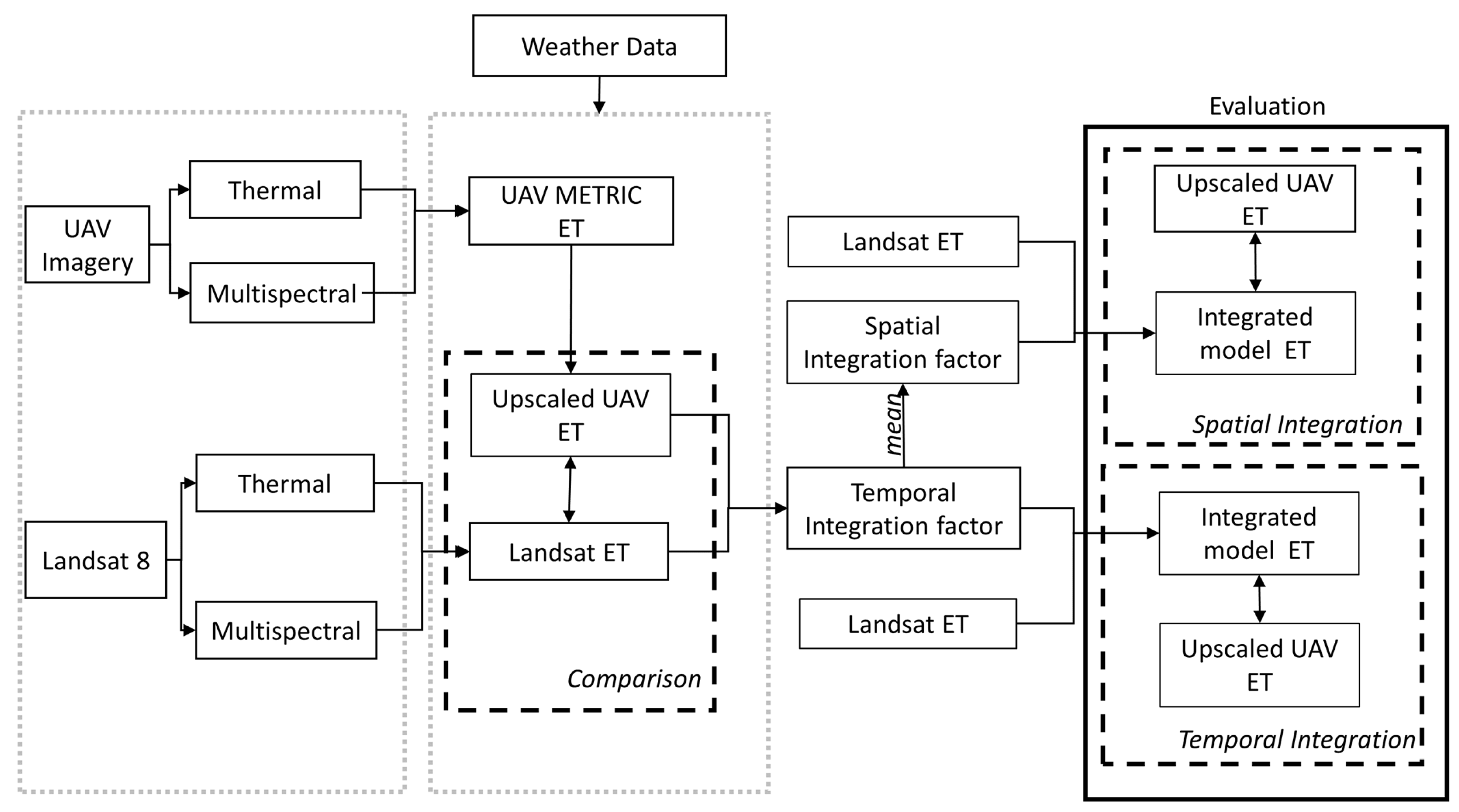
In this study, we propose a method for fusing satellite and UAV ET estimates towards the better prediction of watershed-scale ET estimates. The method employs both temporal and spatial fusion techniques to combine data from the satellite sensor and the UAV using the integration factor. The detailed process used for integration of sensors and model evaluations is shown in Figure 3.

2.7.1. Temporal Integration

We used the temporal integration method for correcting the Landsat ET estimate on day T2 for the same place/crop using the integration factor calculated on day T1. The pixel-by-pixel integration factor (IF) was calculated by taking the ratio of UAV-based ET to Landsat-based ET at day T1 (training day) (Equation (6)).

$${IF}_{temporal}=\frac{{\left({UAV}_{ET}\right)}_{T1}}{{\left({Landsat}_{ET}\right)}_{T1}}$$

(6)

where ${\left({UAV}_{ET}\right)}_{T1}$ is the UAV estimated ET on day T1 and ${\left({Landsat}_{ET}\right)}_{T1}$ is the Landsat estimated ET on day T1. Then the calculated integration factor was multiplied with Landsat ET on day T2 to get the assumed corrected ET (Integrated ET) values on T2 (testing day) (Equation (7)).

$${Integrated}_{ET}={\left({Landsat}_{ET}\right)}_{T2}\times {IF}_{temporal}$$

(7)

where ${Integrated}_{ET}$ is the corrected combination of Landsat and UAV ET on day T2, and ${\left({Landsat}_{ET}\right)}_{T2}$ is Landsat estimated ET on day T2.

For temporal integration, the mapping of the same place with the same crop within a growing season was needed to see how it performed with the correction factor at different times of the year. Since we have these two sets of images only for three crops (alfalfa, peas, and rye grass), the temporal integration is performed only on these crops as farmers rotated corn and wheat with other crops. The details of the sites and days used for integration factor computation and evaluation are provided in

Table 5. Details of the sites used (three crops) for temporal integration factor computation and the testing. Temporal integration factor was calculated using the estimated ET on Training day (T1). Integration and evaluation was done on Testing day (T2).

S.N.	Crop	Site	Training Day Month Year	Testing Day Month Year
1	Peas	Site 10	11 May 2022	21 June 2022
2	Alfalfa	Site 8	11 May 2022	21 June 2022
3	Rye grass	Site 2	12 May 2022	21 June 2022

. Evaluation of the temporal integration factor application was done using the four statistical measures R², RMSE, MAE, and bias.

2.7.2. Spatial Integration

We used the spatial integration method for correcting the Landsat ET estimate at the different place but on same day/crop using the integration factor. The mean value of the pixel-by-pixel integration factor was calculated dividing the UAV ET by the Landsat ET (Equation (8)).

$${IF}_{spatial}=mean\left(\frac{{\left({UAV}_{ET}\right)}_{P1}}{{\left({Landsat}_{ET}\right)}_{P1}}\right)$$

(8)

where ${\left({UAV}_{ET}\right)}_{P1}$ is the UAV estimated ET at site P1, ${\left({Landsat}_{ET}\right)}_{P1}$ is Landsat estimated ET at site P1, and ${IF}_{spatial}$ is the spatial integration factor. Then the calculated mean value of the spatial integration factor was multiplied with Landsat ET at the other site (P2) to get the assumed corrected Landsat ET (Integrated ET) on same day at P2 (testing site) (Equation (9)).

$${Integrated}_{ET}={\left({Landsat}_{ET}\right)}_{P2}\times {IF}_{spatial}$$

(9)

where ${Integrated}_{ET}$ is the corrected combination of Landsat and UAV ET at site P2, and ${\left({Landsat}_{ET}\right)}_{P1}$ is Landsat estimated ET at site P2.

Table 6. Details of the sites (five crops) used for spatial correction factor computation (training) and the testing. Spatial integration factor was calculated using the estimated ET at Training site (P1). Integration and evaluation was done on Testing site (P2).

S.N.	Crop	Day Month Year	Training Site	Testing Site
1	Corn	11 July 2021	Site 1	Site 4
2	Rye grass	11 May 2022	Site 1	Site 2
3	Alfalfa	11 May 2022	Site 4	Site 8
4	Peas	11 May 2022	Site 10	Site 9
5	Wheat	21 June 2022	Site 6	Site 7

details the crop, sites, and days used for the integration factor computation and evaluation. Since R² values do not alter with the division or multiplication by a constant, we evaluated the performance after the application of the spatial integration factor using the RMSE, MAE, and bias statistical measures only.

3. Results

3.1. UAV and Landst Based ET Comparison

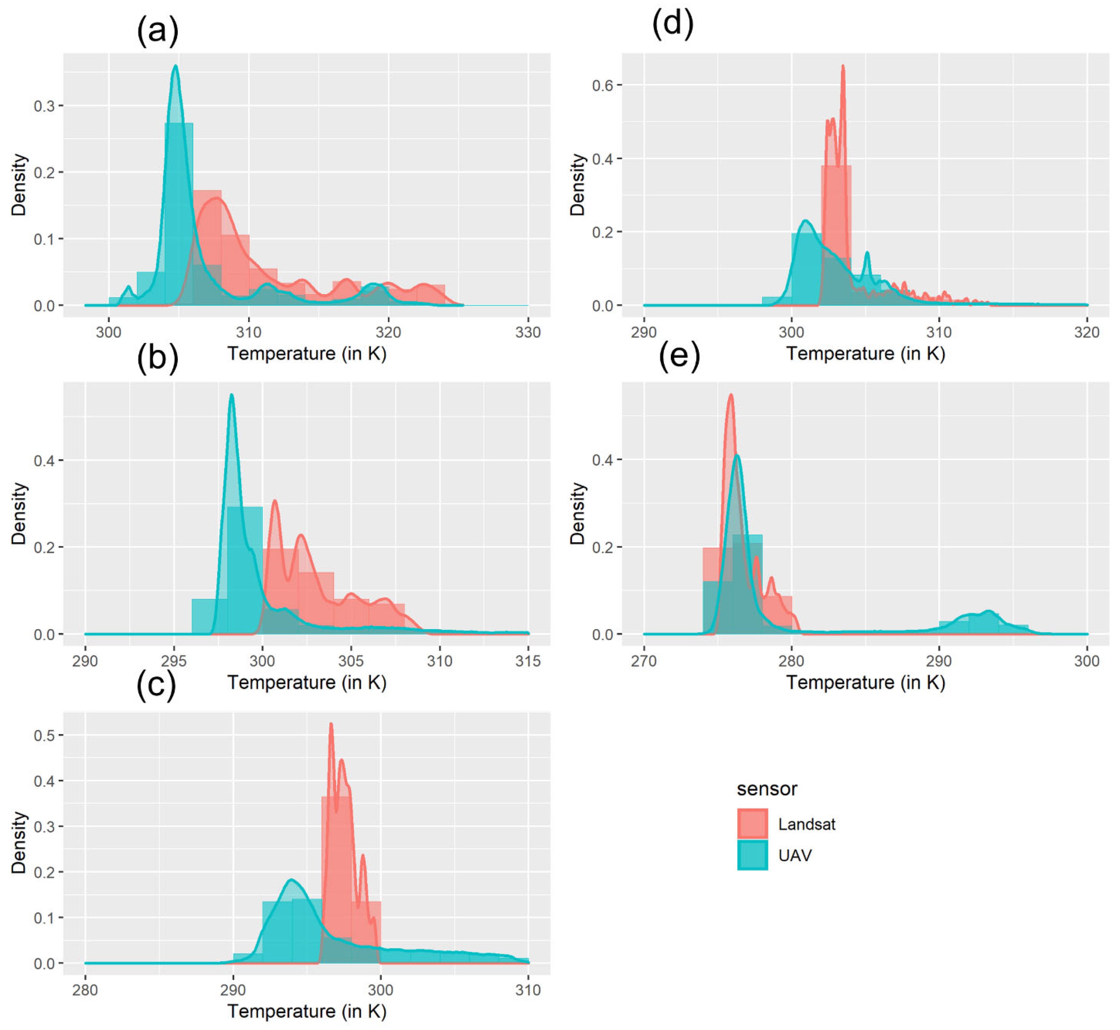
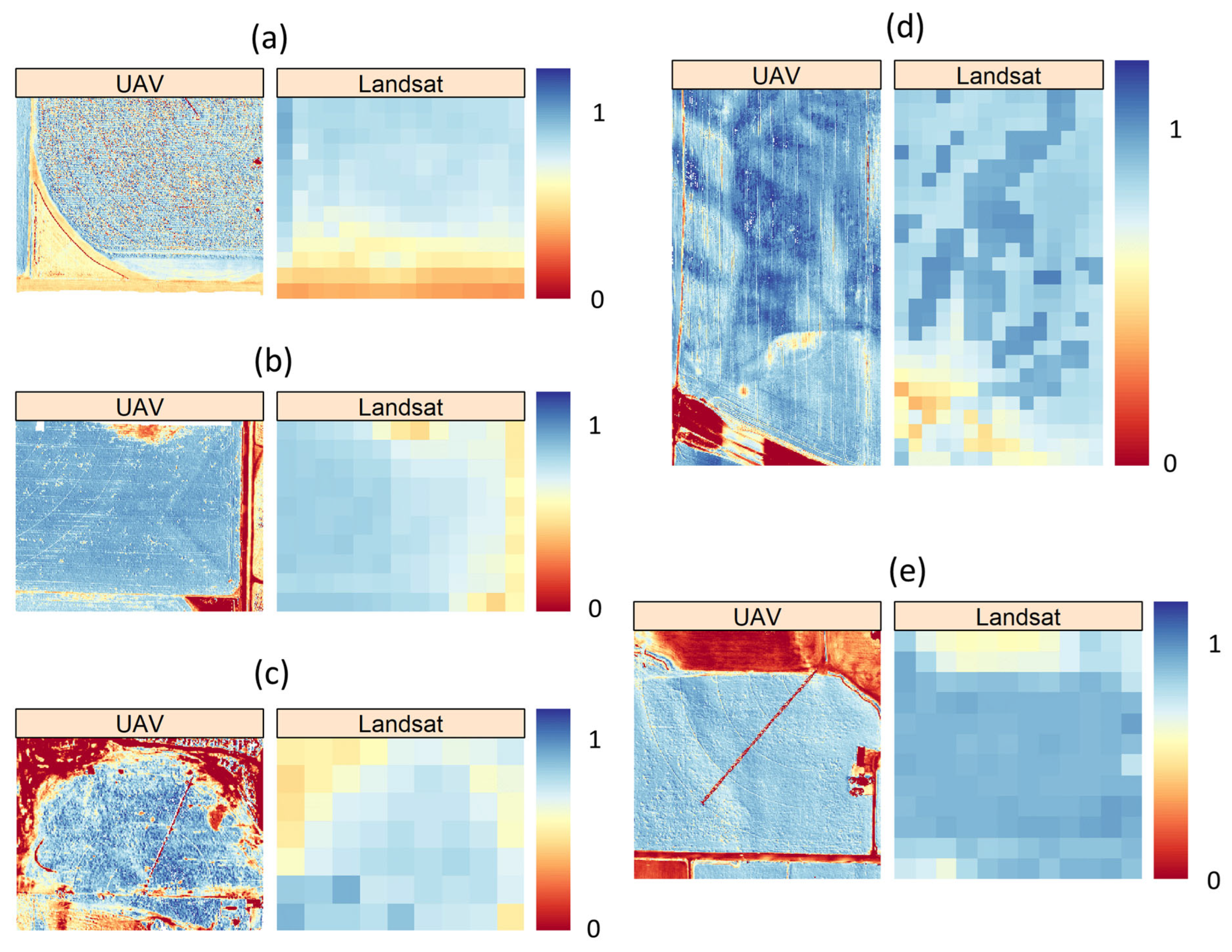
Figure 4 shows the sample mapping of the 24 h ET on five different crops. In line with results from previous studies [43,44], we found an overall similar pattern for ET mapped using both types of imagery. However, detail comparison shows significant spatial variations between barren and highly vegetated areas (

Table 7. Summary statistics of ET on sample five crops across UAV and Landsat sensor at Landsat scale. Min, Max, Mean, Sd represents the minimum, maximum, average, and standard deviation of ET on the corresponding field.

Crop	Day Month Year	UAV (mm/day)				Landsat (mm/day)
		Min	Max	Mean	Sd	Min	Max	Mean	Sd
Corn	11 July 2021	4.73	8.40	7.21	1.02	3.25	9.61	6.97	1.49
Peas	21 June 2022	1.21	6.19	5.33	1.26	2.96	5.66	4.94	0.63
Rye grass	11 May 2022	0.37	5.29	3.40	1.37	2.47	4.96	3.83	0.55
Wheat	21 June 2022	0.1	7.27	5.67	1.25	2.52	6.81	5.35	0.76
Alfalfa	12 May 2022	0.11	2.71	1.99	0.76	1.77	2.88	2.60	0.27

). We found that Landsat consistently overpredicted ET in areas that were relatively bare and underpredicted ET in areas that were covered in vegetation (Figure 4). Overprediction of Landsat ET in bare areas are most noticeable in peas, rye grass, and alfalfa, and underprediction in vegetation areas are most noticeable in wheat. One of the reasons for this variation might be because of varying temperature as the various landscapes exhibit varying temperature differences due to pixel resolution and differing in sensing times. Therefore, we checked the difference between the temperature by plotting the corresponding normalized thermal histogram (Figure 5). Despite the fact that the thermal distribution of both UAV and Landsat is similar (right skewed) for all crops, the median value of UAV-based temperature is lower compared to Landsat. The variation in median value of temperature is due to the differing time of acquisition of UAV and Landsat overpass time (Table 1) as land surface temperature fluctuates significantly during the day, reaching its highest point in the middle of the afternoon, which might have led to the some noticeable variation in ET [45].

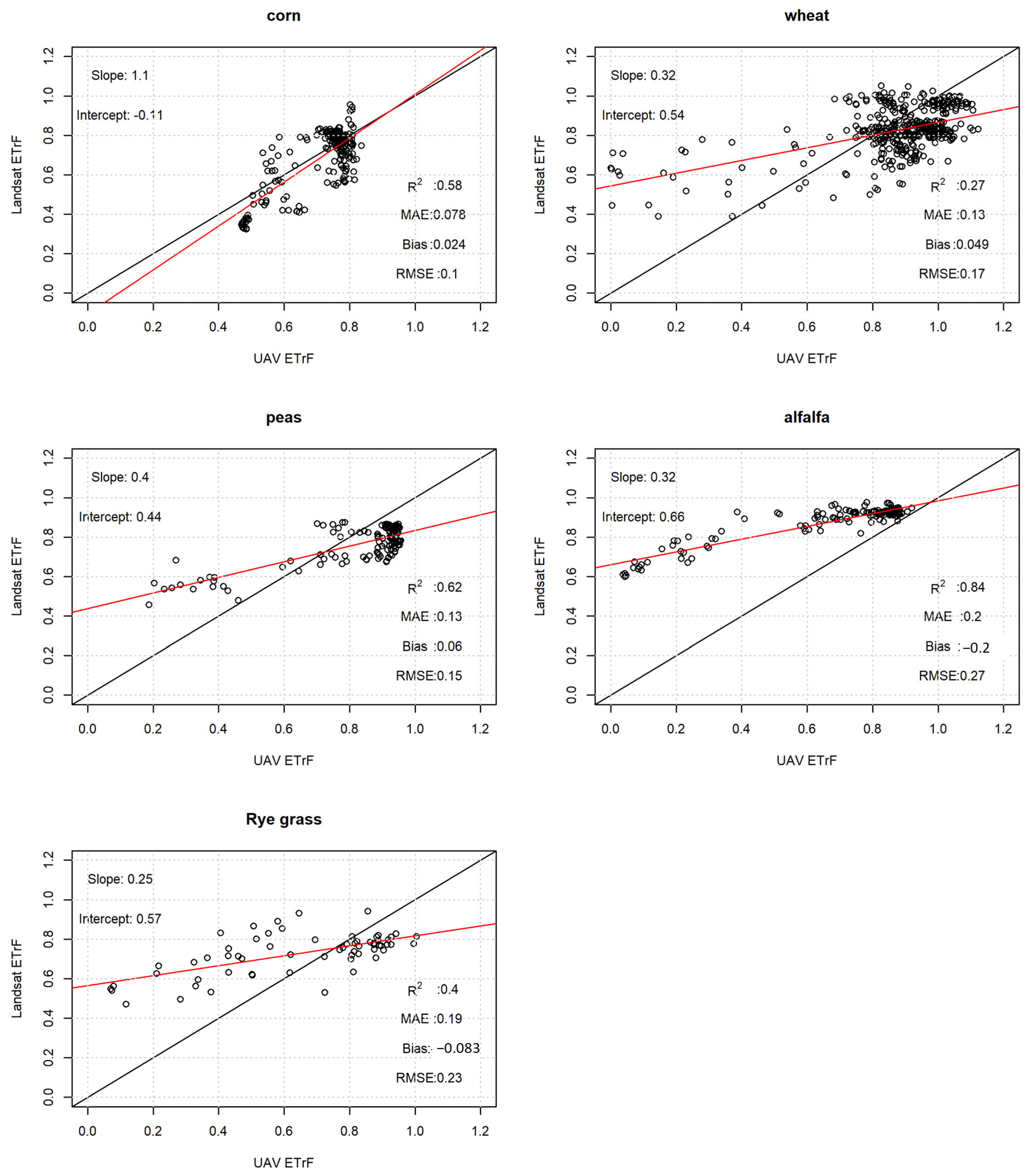
3.2. Statistical Comparison of Fractional Evapotranspiration (ETrF)

While comparison of daily evapotranspiration shows how crop ET varies on a particular day, the comparison of fractional evapotranspiration (ETrF), which is the ratio of actual ET to reference ET, is easier for evaluating how it performs across different crops within the same scale. Figure 6 shows scatterplots between sample aggregated UAV and Landsat ETrF (one for each crop) whereas

Table 8. Statistical measure of the relationship between fractional evapotranspiration mapped using the Landsat and UAV imagery at 30 m resolution for each day of Landsat overpass on five crops.

Crop	Day Month Year	R2	RMSE	MAE	Bias
Alfalfa	11 July 2021	0.64	0.15	0.06	0.04
	11 May 2022	0.64	0.24	0.22	−0.21
	12 May 2022	0.84	0.27	0.20	−0.20
	21 June 2022	0.69	0.12	0.10	0.03
Wheat	11 July 2021	0.68	0.10	0.12	0.10
	21 June 2022	0.27	0.17	0.13	0.05
Rye grass	11 May 2022	0.40	0.23	0.19	−0.08
	12 May 2022	0.40	0.20	0.19	−0.21
	21 June 2022	0.46	0.12	0.10	−0.09
Peas	11 May 2022	0.49	0.19	0.18	−0.17
	21 June 2022	0.62	0.15	0.13	0.06
Corn	11 July 2021	0.58	0.10	0.08	0.02

shows the statistical comparison at each overpass date at a 30 m resolution. Overall, we found the R² values in the range of 0.27 to 0.84 comparable with the aggregated aerial temperature and Landsat temperature comparison [44]. RMSE and MAE ranged from 0.1 to 0.27 and 0.06 to 0.22, respectively. Similarly, the bias ranges from −0.21 to 0.2, where the positive bias imply that the ETrF obtained from the Landsat images were overestimated, whereas negative bias suggests that the ETrF values were underestimated from those obtained from UAV images.

Evaluated by crop, alfalfa (0.64–0.84), peas (0.49–0.62), corn (0.58), rye grass (0.4–0.46), and wheat (0.27–0.68) showed an excellent R² (0.4) with the exception of wheat on 21 June 2022. A major factor responsible for low R² values for wheat on 21 June 2022 is the concentration of most of the ETrF values in the range of 0.8 to 1.1, with few below 0.8, as it was the peak stage of water consumption for wheat, giving higher ET values. This can be further verified from the RMSE values, which is just 0.17 in the case of wheat whereas RMSE is 0.27 in the case of alfalfa which has the good R² value of 0.84. Although good correlation was found, there is a significant bias (alfalfa: −0.21 to 0.03, wheat: 0.05 to 0.1, rye grass: −0.21 to −0.08, peas: −0.17, 0.06, corn: 0.02) in the ETrF mapped using UAV and Landsat imagery. The positive biases for wheat on 11 July 2021 and 21 June 2022 implies the EtrF values obtained from the Landsat images were overestimated, whereas negative biases for rye grass on 11 May, 12 May, and 21 June 2022 suggests that the temperature values were slightly deviating from those obtained from UAV images. We also found that if the UAV technique is employed as benchmark, Landsat data exhibit a propensity to exaggerate low values and underestimate high values. While the exact cause of this error needs to be further investigated, it may be due to the Landsat thermal band’s inferior resolution at 100 m. Although this data is processed and reduced to 30 m, the averaging may result in ET estimates that were different than the UAV estimates, as land surface temperature is a key element in determining ET using METRIC method. For successful integration of ET obtained from UAV and Landsat images we need estimation of the integration factors. As seen from the Figure 6 (slope and intercept), there are unique relationships between the ET mapped using UAV imagery for each crop and the ET mapped using Landsat imagery. These findings hint that each crop has a distinct connection, and that the integration of the ET mapped using these sensors requires distinct integration factors.

3.3. Variability of ETrF

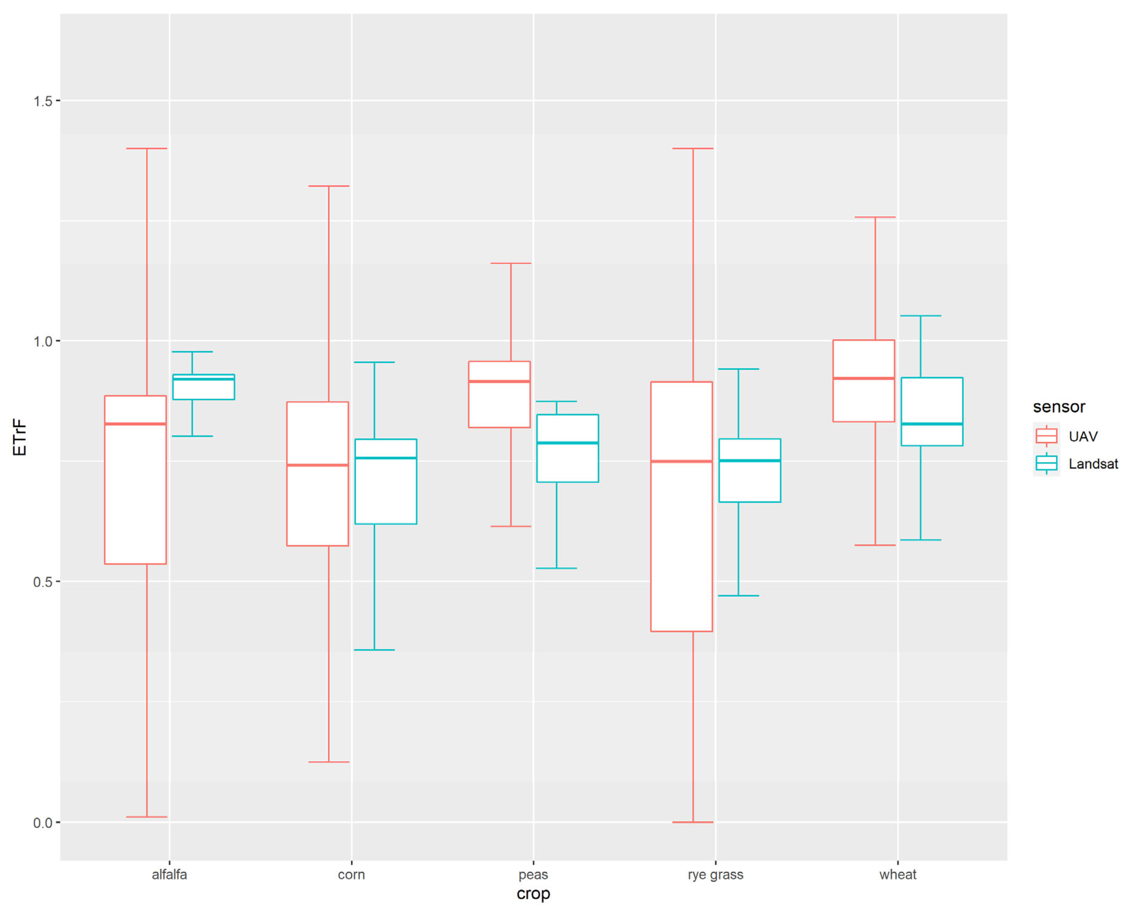
The spatial variability of ETrF captured by the UAV and Landsat modeling approaches on sample sites are shown in Figure 7. As pixel sizes are small for the UAV compared to Landsat, more variability is captured. The information regarding variability of water demand is crucial for the better management of water in precision agriculture including the application of variable irrigation [46,47,48]. From Figure 8 we can infer that the median values of fractional ETrF do not show any trend of ET variation. Alfalfa and wheat have greater median ETrF values for Landsat, while peas have lower values. On maize and rye grass, the median ETrF values predicted by both sensors are comparable. The Figure 8 shows much more variability across the field on two crops of alfalfa and on rye whereas show less variability in the case of peas and wheat. This is because there were constant applications of irrigation on alfalfa and rye with some part remaining to irrigate whereas, irrigation was just turned off after complete application on wheat and peas.

3.4. Partial Cloud Effect on UAV-ET

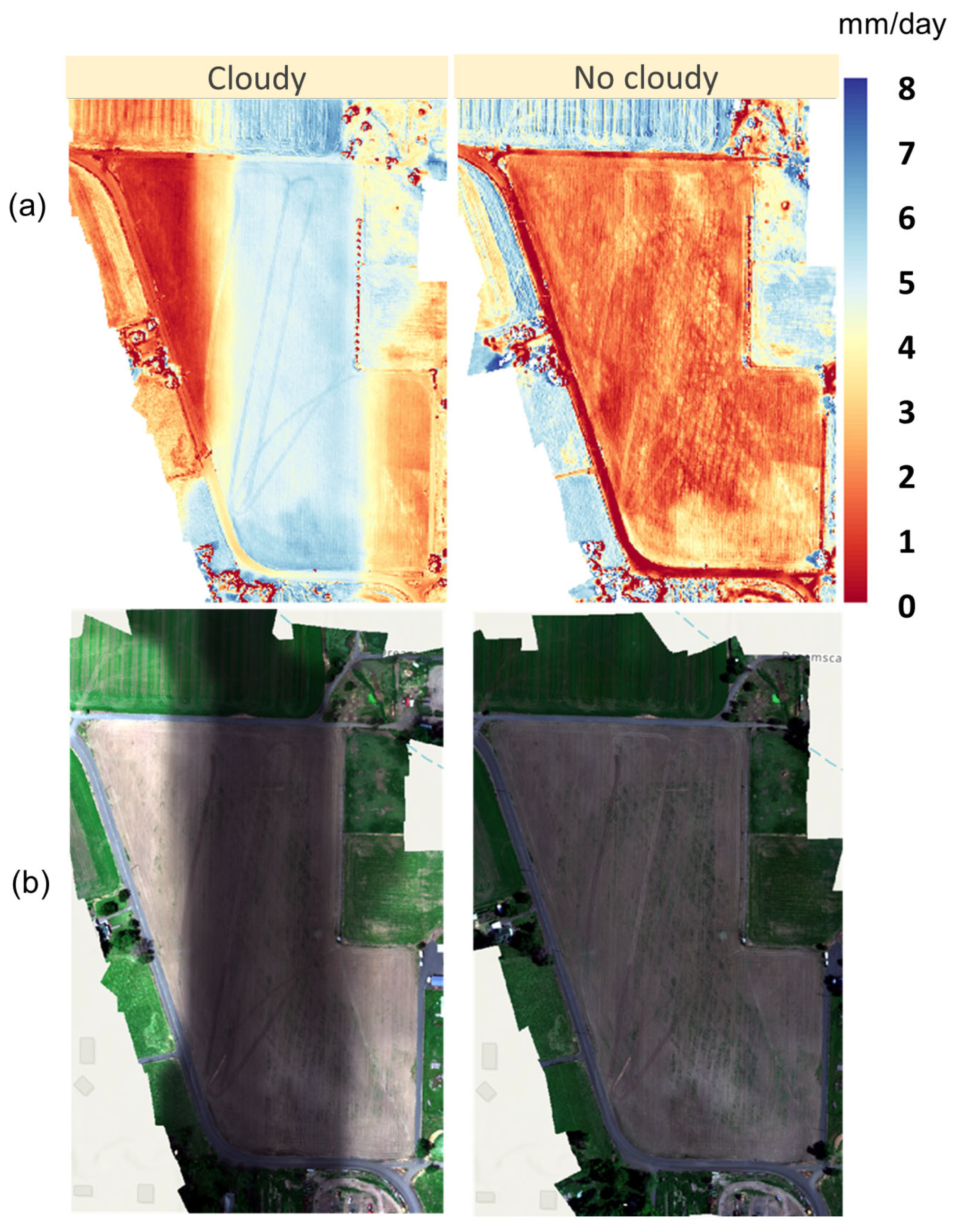
Figure 9 below shows the UAV ET mapping for a cornfield at site3 on the same day but at different times under partial cloud and cloud free conditions. It shows that the predicted evapotranspiration is higher in places superimposed by cloud shadows than in other cloud-free places. This is because the pixel overlaid over cloud shadows resulted in lesser LST values giving the weaker longwave radiation from the ground based on the Stefan-Boltzman equation. As a result, in comparison to the pixels in the non-cloudy areas, the net radiation (and subsequently the predicted ET) of the pixels overlaid under cloud shadows increased more than the ET, which was unexpected. Direct comparison between the two images shows that the ET mapped are almost similar in places other than the overcast cloud shadows. Therefore, although the UAV can be flown under the cloudy conditions, there seems to be a direct influence on the ET estimation that needs to be accounted for especially during partly cloudy sampling.

3.5. Temporal Integration of ET

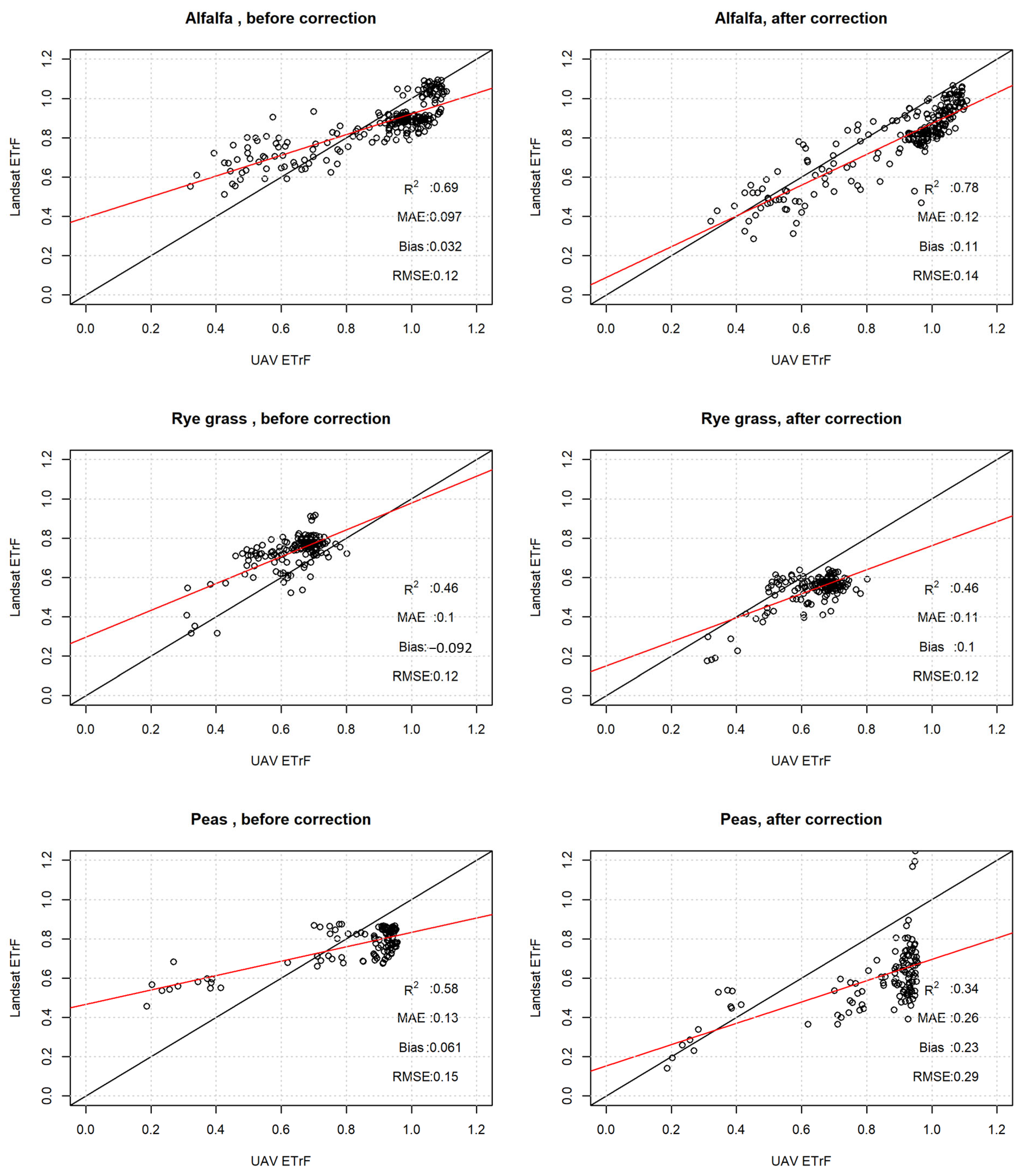
Since 24-h ET estimated by two sensors departs from each other, it raises the question of whether ET estimated using these two sensors can be combined for time series integration. To answer this question, we compared the ET estimated using the UAV imagery with ET estimated using the Landsat imagery with and without the application of the integration factor. For time series integration, we need to map the same place with the same crop within a growing season to see how it behaves at different times of the year. As we have needed two sets of images for three crops only, the comparison results presented here are based on these three crops. The pixel-by-pixel integration factor was calculated by dividing the UAV predicted ETrF by Landsat predicted ETrF on 11 May and 12 May, and thus the calculated integration factor was applied to get the corrected ET values on 21 June of 2022. Interestingly, the integration assessment revealed that the application of the integration factor for time series integration depends upon the plant’s growth stage and the irrigation water application (Figure 10). This becomes more evident from the comparison of relationship of alfalfa and peas, where R² values significantly improve with the application of the integration factor from 0.69 to 0.78 whereas it decreases in the case of peas from 0.58 to 0.34. One reason that leads to such variation between these two crops is that alfalfa was being irrigated during both flights, whereas the peas were not irrigated at the first image and was irrigated later. This might be also because the METRIC ET at the early stage of the crop growth is not good and the integration factor calculated using this crop at an early stage might not work for the later stage of the crop. Similarly, we can see that there is no variation on R² for the rye grass with and without the application of the correction factor, which might be because this field was constantly irrigated and cow calves were constantly grazed, making these two situations not ideal. Thus, the application of the correction factor has no meaning here. Therefore, based on this result we can infer that for the time series integration, the integration factor from one image to another can be done if they are in a similar growth stage and have similar irrigation applications.

3.6. Spatial Integration of ET

As temporal integration did not show any constant pattern of improvement with the use of integration factors, we further examined whether these ET estimates could be integrated spatially by the application of integration factors. Since the pixel-by-pixel correlation factor cannot be applied for ET computation at other sites as in previous steps, here we computed the mean value of the integration factor.

Table 9. Spatial integration factors for five crops in the descending order.

S.N.	Crop	Day Month Year	Integration Factor
1	Wheat	21 June 2022	1.19
2	Rye grass	11 May 2022	0.87
3	Alfalfa	11 May 2022	0.75
4	Corn	11 July 2021	0.84
5	Peas	11 May 2022	0.65

shows the mean values of the integration factor, calculated using these two sensors on all five crops on the particular day listed below. The integration factors were found in the increasing order from peas, alfalfa, corn, rye grass, and wheat. The highest integration factor on wheat might be because the Landsat predicts a relatively low value of ET on dense vegetation areas compared to UAV ET. Similarly, the lowest integration factor of 0.65 on peas was also because the Landsat predicts relatively high values on bare areas compared to UAV ET. The integration factor for alfalfa and peas calculated on the same day have different values, based on this result we can say that the integration factor is unique for each crop even on a single day.

While Figure 11 depicts the comparison raster plot of ET across sensors,

Table 10. Summary of statistical measure (root mean square error, mean absolute error, and bias) with and without the application of integration factor.

S.N.	Crop	Before Integration (mm/day)			After Integration (mm/day)
		RMSE	MAE	Bias	RMSE	MAE	Bias
1	Wheat	1.71	1.56	1.55	0.91	0.76	0.49
2	Rye grass	1.30	1.27	−1.26	0.72	0.65	−0.64
3	Alfalfa	1.22	1.15	−1.15	0.42	0.30	0.16
4	Corn	1.60	1.30	−1.27	1.03	0.76	−0.32
5	Peas	2.63	2.55	−2.55	1.14	1.09	−0.91

summarizes the change in statistical values with and without the application of integration factors on hold out set. Our result shows that the METRIC ET predicted using Landsat will be significantly decreased with the application of integration factor RMSE (35.75% to 65.52%), MAE (41.99% to 73.81%), bias (49.56% to 85.85%). Evaluated by crop, the highest improvements were found in alfalfa with the RMSE (1.22 to 0.42), MAE (1.15 to 0.3), and bias (−1.15 to 0.16), whereas the lowest improvement was found on the corn with RMSE (1.6 to 1.03), MAE (1.3 to 0.76). Since the mean value of the correction was applied, this might be because there was less variability in ET for alfalfa compared to the corn. Similarly, we found the improvement greater than 45% on all RMSE, MAE, and bias values for other crops of rye grass, wheat, and peas. Based on the Figure 11 and the Table 10 it is conceivable that the integration factor computed at one location for a crop can be applied at the other location and this will help in the better prediction of the watershed scale ET.

4. Discussion

4.1. Comparison of Total ET

Integration of sensors is a cost-effective way of mapping earth observations with the fusion of satellite and UAV images becoming increasingly popular [20,49,50]. A positive correlation between Landsat predicted and UAV predicted seasonal ET has been shown [19,43]. Since daily ET estimation is critical for effective water management, in this study the METRIC model was used for comparing and integrating the daily ET. We first demonstrated that Landsat estimated 24 h ET was positively correlated with the UAV ET with the coefficient of determination in the range of 0.27–0.84, consistent with the literature on seasonal ET comparison [43,44]. In particular, the median values of ET for a field was similar (Figure 5), forming the base for the integration of sensors.

Since UAV-based ET mapping incurs a certain extra cost for water managers [51], we further asked whether there is a sizeable difference in ET mapped using UAV versus satellite imagery. Our result shows that although the median values are similar and positively correlated, the Landsat ET and UAV ET vary across the field (Figure 7), resulting in a change in the total water budget. We found that the total water budget can vary up to 114 m³ (wheat: 114 m³ for an area of 36.45 hectares, alfalfa: 78 m³ for an area of 12.96 hectares, corn: 43 m³ for an area of 18.72 hectares, rye grass: 25 m³ for an area of 5.67 hectares, and peas: 45 m³ for an area of 11.7 hectares). Besides, Landsat ET is normally over-predicted around bare land areas and under-predicted around the dense vegetation areas compared to UAV ET (Figure 4). The reason for this difference is due to the varying sensing time and pixel resolution as the various landscapes exhibit varying temperature and ET results are influenced by the aggregation [44,45,52]. As ET mapped using UAV-based imagery was done at higher spatial resolution, the variability in ET captured using UAV imagery is higher compared to Landsat imagery. Thus, the UAV approach of ET estimation supersedes the Landsat approach for their application in precision agriculture such as identifying ponding locations, identifying water stress or overirrigation at the field size, and identifying irrigation system malfunctions [46,47,48]. Therefore, our results indicate that this difference in ET variability across two sensors warrant the further investment in UAV-based image mapping for field scale evaluation.

4.2. Cloud Cover Effect

We also assessed the possible cloud impact on UAV based ET estimation. As illustrated in Figure 9, additional precautions are needed for ET mapping using UAV imagery as cloud-based illumination impedes the ET estimation from the field. Although the UAV can be flown under the clouds [46,53], the shadows cast by the clouds appear to have a direct influence on ET estimation. The timing for UAV flying to determine the ET from the field is thus constrained. Further research and investments are required to check whether there is an effect under partial cloud only or when we have full cloud conditions.

4.3. Integration of ET

We examined if there is a way to combine these two sensors for better prediction of ET. Similar to other remote sensing integration applications [52,54,55], our spatial integration result shows that the Landsat ET can be used in synergy with UAV ET. We found that the RMSE, MAE, and bias values are significantly reduced in all crops by the application of the integration factor by at least 35.75% (Table 10). This work will not only reduce the reliability of people on single satellite-based imagery or UAV-based imagery for the computation of the watershed scale ET, but will also significantly reduce the operational cost of UAV image acquisition as only fewer flights are needed for the computation of the integration factor. Therefore, the computation of an integration factor is crucial for the successful integration of these two sensors. Once the integration factor is computed it can be applied to the Landsat based ET. Additionally, our results provide evidence that ET estimation would benefit from the synergy of UAV imagery with Landsat imagery for mapping ET at a watershed scale as they can complement each other in their ET prediction.

In contrast to the spatial integration, temporal integration shows the mix result for UAV ET integration with Landsat ET. We computed the integration factor using the image collected on May of 2022, which was applied with the image collected on June 2022. The purpose was to see if we could apply the same pixel by pixel integration factor at a place for a crop within the same growing season as done in other spatiotemporal studies [55,56]. We found mixed results in alfalfa, with R² values significantly increased from 0.69 to 0.78 with a small reduction in RMSE and MAE values, whereas all R², RMSE, and MAE values did not improve by using such an integration factor on peas and rye grass (Figure 10). This suggests that the pixel by pixel factor can only be applied if the crop’s growth stage does not differ a lot and if there is similar application of irrigation with less variation in hydrothermal condition similar to the study on crop landscape [57,58].

This study is the first step in identifying a possible integration factor for the use of Landsat ET in combination with UAV ET. The data suggest that with the integration factor Landsat ET can be used in synergy with the UAV ET for a better prediction of watershed scale ET. Understanding these earlier steps of ET integration provide a novel approach in using the satellite of ET with UAV ET, which may ultimately lead to effective field and watershed scale water management. This work will reduce people’s reliability on a single satellite or UAV-based imagery for the computation of the watershed scale ET. It is also conceivable that such a method of integration could work in many other crops including annual and perennial crops, as well as for many other types of satellite and UAV sensors.

Finally, it is crucial to acknowledge a number of critical decision-making processes that were considered beyond the scope of the current project. UAV-based ET was utilized in this work to correct Landsat-based ET, however no ground observations were used to determine the accuracy of UAV-based ET because of the lack of Eddy Covariance stations in our study. Further, we used the same equations for the broadband albedo estimation from the narrow band without considering the crop growth stage. However, as pointed out by Bartmiński and Siłuch [52], the surface albedo equation needs adjustment for crop growth stage. Besides, the current study was performed on working fields (not experimental plots) allowing the farmers to use their own management practice, irrigation application, and crop rotation. While this may make the study better for real world approximation, it hinders the research as we could not get the corn crop in the same field for two consecutive years. Future work could address these dimensions, as well as formulating a more complex integration model that accounts for the change in crop growth stage and variation across the annual and perennial crop. Comparing integrated ET along with UAV and satellite-based ET with Eddy Covariance stations could also provide additional insight.

5. Conclusions

We have estimated and analyzed daily ET values using two different remote sensing platforms typically used for earth observations. Pixel-by-pixel comparison suggest that the daily ET estimates have varying degrees of coefficient of determination in the range of 0.27 to 0.84 depending upon crop types. The UAV-based ET estimates exhibit higher variability in ET and can provide real time ET estimation that has a heightened interest for routine monitoring of daily ET and surface energy fluxes. Thus, UAV-based ET estimates are crucial for the real time ET estimation. Moreover, the similarity in the median value of the ET mapped by two sensors and the positive correlation suggest that integrating these two methods may provide a good earth observation like in similar applications. The initial proof-of-concept experiment demonstrates that the combination of these two sensors will improve ET prediction and that the errors are greatly reduced when an integration factor is applied. The possibility of integrating two sources of ET estimates with the application of an integration factor provides the additional justification for the investment in UAV based consumptive use measurements and monitoring—a critical element for water markets in the western United States. This will help reduce costs, as mapping the entire watershed is not required, and for same day mapping the integration factor computed at one location can be applied to a similar crop within the watershed. Further application of this integration of UAV ET with Landsat ET will help better predict watershed scale ET, thereby increasing our understanding of demand and availability of water for effective water management.

References

- Vörösmarty, C.J.; Green, P.; Salisbury, J.; Lammers, R.B. Global Water Resources: Vulnerability from Climate Change and Population Growth. Science 2000, 289, 284. [Google Scholar] [CrossRef]
- Scanlon, B.R.; Faunt, C.C.; Longuevergne, L.; Reedy, R.C.; Alley, W.M.; McGuire, V.L.; McMahon, P.B. Groundwater depletion and sustainability of irrigation in the US High Plains and Central Valley. Proc. Natl. Acad. Sci. USA 2012, 109, 9320. [Google Scholar] [CrossRef]
- Flörke, M.; Schneider, C.; McDonald, R.I. Water competition between cities and agriculture driven by climate change and urban growth. Nat. Sustain. 2018, 1, 51–58. [Google Scholar] [CrossRef]
- Khanal, R.; Brady, M.P.; Stöckle, C.O.; Rajagopalan, K.; Yoder, J.; Barber, M.E. The Economic and Environmental Benefits of Partial Leasing of Agricultural Water Rights. Water Resour. Res. 2021, 57, e2021WR029712. [Google Scholar] [CrossRef]
- Schaible, G.; Aillery, M. Water Conservation in Irrigated Agriculture: Trends and Challenges in the Face of Emerging Demands. SSRN Electron. J. 2012. [Google Scholar] [CrossRef]
- D’Odorico, P.; Chiarelli, D.; Rosa, L.; Bini, A.; Zilberman, D.; Rulli, M.C. The global value of water in agriculture. Proc. Natl. Acad. Sci. USA 2020, 117, 21985–21993. [Google Scholar] [CrossRef] [PubMed]
- Khanal, R.; Barber, M. Modeling Water Leasing Impacts on Instream Flows for River Ecosystem Protection. In Proceedings of the AGU Fall Meeting 2021, New Orleans, LA, USA, 13–17 December 2021; Volume 2021, p. H35Q-1231. [Google Scholar]
- Caselles, V.; Sobrino, J.; Coll, C. On the use of satellite thermal data for determining evapotranspiration in partially vegetated areas. Int. J. Remote Sens. 1992, 13, 2669–2682. [Google Scholar] [CrossRef]
- Kustas, W.; Norman, J. Use of remote sensing for evapotranspiration monitoring over land surfaces. Hydrol. Sci. J. 1996, 41, 495–516. [Google Scholar] [CrossRef]
- Zhang, Y.; Peña-Arancibia, J.L.; McVicar, T.R.; Chiew, F.H.S.; Vaze, J.; Liu, C.; Lu, X.; Zheng, H.; Wang, Y.; Liu, Y.Y.; et al. Multi-decadal trends in global terrestrial evapotranspiration and its components. Sci. Rep. 2016, 6, 19124. [Google Scholar] [CrossRef]
- Jung, M.; Reichstein, M.; Margolis, H.A.; Cescatti, A.; Richardson, A.D.; Arain, M.A.; Arneth, A.; Bernhofer, C.; Bonal, D.; Chen, J.; et al. Global patterns of land-atmosphere fluxes of carbon dioxide, latent heat, and sensible heat derived from eddy covariance, satellite, and meteorological observations. J. Geophys. Res. Biogeosci. 2011, 116. [Google Scholar] [CrossRef]
- Dhungel, S.; Barber, M.E. Estimating Calibration Variability in Evapotranspiration Derived from a Satellite-Based Energy Balance Model. Remote Sens. 2018, 10, 1695. [Google Scholar] [CrossRef]
- Koch, J.; Zhang, W.; Martinsen, G.; He, X.; Stisen, S. Estimating Net Irrigation Across the North China Plain Through Dual Modeling of Evapotranspiration. Water Resour. Res. 2020, 56, e2020WR027413. [Google Scholar] [CrossRef]
- Zhang, K.; Kimball, J.S.; Running, S.W. A review of remote sensing based actual evapotranspiration estimation. WIREs Water 2016, 3, 834–853. [Google Scholar] [CrossRef]
- Bellvert, J.; Adeline, K.; Baram, S.; Pierce, L.; Sanden, B.L.; Smart, D.R. Monitoring Crop Evapotranspiration and Crop Coefficients over an Almond and Pistachio Orchard Throughout Remote Sensing. Remote Sens. 2018, 10, 2001. [Google Scholar] [CrossRef]
- Jia, D.; Cheng, C.; Song, C.; Shen, S.; Ning, L.; Zhang, T. A Hybrid Deep Learning-Based Spatiotemporal Fusion Method for Combining Satellite Images with Different Resolutions. Remote Sens. 2021, 13, 645. [Google Scholar] [CrossRef]
- Feng, G.; Masek, J.; Schwaller, M.; Hall, F. On the blending of the Landsat and MODIS surface reflectance: Predicting daily Landsat surface reflectance. IEEE Trans. Geosci. Remote Sens. 2006, 44, 2207–2218. [Google Scholar] [CrossRef]
- Ma, X.; Sanguinet, K.A.; Jacoby, P.W. Direct root-zone irrigation outperforms surface drip irrigation for grape yield and crop water use efficiency while restricting root growth. Agric. Water Manag. 2020, 231, 105993. [Google Scholar] [CrossRef]
- Chandel, A.K.; Khot, L.R.; Molaei, B.; Peters, R.T.; Stöckle, C.O.; Jacoby, P.W. High-Resolution Spatiotemporal Water Use Mapping of Surface and Direct-Root-Zone Drip-Irrigated Grapevines Using UAS-Based Thermal and Multispectral Remote Sensing. Remote Sens. 2021, 13, 954. [Google Scholar] [CrossRef]
- Mokhtari, A.; Ahmadi, A.; Daccache, A.; Drechsler, K. Actual Evapotranspiration from UAV Images: A Multi-Sensor Data Fusion Approach. Remote Sens. 2021, 13, 2315. [Google Scholar] [CrossRef]
- Backes, D.J.; Teferle, F.N. Multiscale Integration of High-Resolution Spaceborne and Drone-Based Imagery for a High-Accuracy Digital Elevation Model Over Tristan da Cunha. Front. Earth Sci. 2020, 8, 319. [Google Scholar] [CrossRef]
- Díaz-Varela, R.A.; De la Rosa, R.; León, L.; Zarco-Tejada, P.J. High-Resolution Airborne UAV Imagery to Assess Olive Tree Crown Parameters Using 3D Photo Reconstruction: Application in Breeding Trials. Remote Sens. 2015, 7, 4213–4232. [Google Scholar] [CrossRef]
- Ortega-Farías, S.; Ortega-Salazar, S.; Poblete, T.; Kilic, A.; Allen, R.; Poblete-Echeverría, C.; Ahumada-Orellana, L.; Zuñiga, M.; Sepúlveda, D. Estimation of Energy Balance Components over a Drip-Irrigated Olive Orchard Using Thermal and Multispectral Cameras Placed on a Helicopter-Based Unmanned Aerial Vehicle (UAV). Remote Sens. 2016, 8, 638. [Google Scholar] [CrossRef]
- Gautam, D.; Ostendorf, B.; Pagay, V. Estimation of Grapevine Crop Coefficient Using a Multispectral Camera on an Unmanned Aerial Vehicle. Remote Sens. 2021, 13, 2639. [Google Scholar] [CrossRef]
- Pearson, W.A. Drones in Precision Agriculture: Corn Field Testing and Sampling through Drone Mapping; California State University: Frenso, CA, USA, 2018. [Google Scholar]
- Colomina, I.; Molina, P. Unmanned aerial systems for photogrammetry and remote sensing: A review. ISPRS J. Photogramm. Remote Sens. 2014, 92, 79–97. [Google Scholar] [CrossRef]
- Xia, T.; Kustas, W.P.; Anderson, M.C.; Alfieri, J.G.; Gao, F.; McKee, L.; Prueger, J.H.; Geli, H.M.E.; Neale, C.M.U.; Sanchez, L.; et al. Mapping evapotranspiration with high-resolution aircraft imagery over vineyards using one- and two-source modeling schemes. Hydrol. Earth Syst. Sci. 2016, 20, 1523–1545. [Google Scholar] [CrossRef]
- Qin, L.; Yan, C.; Yu, L.; Chai, M.; Wang, B.; Hayat, M.; Shi, Z.; Gao, H.; Jiang, X.; Xiong, B.; et al. High-resolution spatio-temporal characteristics of urban evapotranspiration measured by unmanned aerial vehicle and infrared remote sensing. Build. Environ. 2022, 222, 109389. [Google Scholar] [CrossRef]
- Gray, P.C.; Ridge, J.T.; Poulin, S.K.; Seymour, A.C.; Schwantes, A.M.; Swenson, J.J.; Johnston, D.W. Integrating Drone Imagery into High Resolution Satellite Remote Sensing Assessments of Estuarine Environments. Remote Sens. 2018, 10, 1257. [Google Scholar] [CrossRef]
- Bhatnagar, S.; Gill, L.; Regan, S.; Waldren, S.; Ghosh, B. A nested drone-satellite approach to monitoring the ecological conditions of wetlands. ISPRS J. Photogramm. Remote Sens. 2021, 174, 151–165. [Google Scholar] [CrossRef]
- Niu, H.; Hollenbeck, D.; Zhao, T.; Wang, D.; Chen, Y. Evapotranspiration Estimation with Small UAVs in Precision Agriculture. Sensors 2020, 20, 6427. [Google Scholar] [CrossRef]
- Mokari, E.; Samani, Z.; Heerema, R.; Dehghan-Niri, E.; DuBois, D.; Ward, F.; Pierce, C. Development of a new UAV-thermal imaging based model for estimating pecan evapotranspiration. Comput. Electron. Agric. 2022, 194, 106752. [Google Scholar] [CrossRef]
- R Core Team. R: A Language and Environment for Statistical Computing 2020; Foundation for Statistical Computing: Vienna, Austria, 2019. [Google Scholar]
- MicaSense. What Are the Units of the Atlas Geo TIFF Output? Available online: https://support.micasense.com/hc/en-us/articles/215460518-What-are-the-units-of-the-Atlas-GeoTIFF-output- (accessed on 16 September 2022).
- MicaSense. Converting Altum Thermal to Degrees C after Processing in Agisoft or Pix4D. Available online: https://support.micasense.com/hc/en-us/articles/360022446473-Converting-Altum-Thermal-to-degrees-C-after-processing-in-Agisoft-or-Pix4D (accessed on 16 September 2022).
- Allen, R.G.; Tasumi, M.; Morse, A.; Trezza, R. A Landsat-based energy balance and evapotranspiration model in Western US water rights regulation and planning. Irrig. Drain. Syst. 2005, 19, 251–268. [Google Scholar] [CrossRef]
- Liaqat, U.; Choi, M. Surface energy fluxes in the Northeast Asia ecosystem: SEBS and METRIC models using Landsat satellite images. Agric. For. Meteorol. 2015, 214–215, 60–79. [Google Scholar] [CrossRef]
- Khanal, R.; Dhungel, S.; Brewer, S.C.; Barber, M.E. Statistical Modeling to Predict Climate Change Effects on Watershed Scale Evapotranspiration. Atmosphere 2021, 12, 1565. [Google Scholar] [CrossRef]
- Allen, R.G.; Tasumi, M.; Trezza, R. Satellite-Based Energy Balance for Mapping Evapotranspiration with Internalized Calibration (METRIC)—Model. J. Irrig. Drain. Eng. 2007, 133, 380–394. [Google Scholar] [CrossRef]
- Brest, C.L.; Goward, S.N. Deriving surface albedo measurements from narrow band satellite data. Int. J. Remote Sens. 1987, 8, 351–367. [Google Scholar] [CrossRef]
- Olmedo, G.F.; Ortega-Farías, S.; de la Fuente-Sáiz, D.; Fonseca-Luego, D.; Fuentes-Peñailillo, F. Water: Tools and Functions to Estimate Actual Evapotranspiration Using Land Surface Energy Balance Models in R. R J. 2016, 8, 352–369. [Google Scholar] [CrossRef]
- Molaei, B.; Peters, R.T.; Khot, L.R.; Stöckle, C.O. Assessing Suitability of Auto-Selection of Hot and Cold Anchor Pixels of the UAS-METRIC Model for Developing Crop Water Use Maps. Remote Sens. 2022, 14, 4454. [Google Scholar] [CrossRef]
- Chandel, A.K.; Molaei, B.; Khot, L.R.; Peters, R.T.; Stöckle, C.O. High Resolution Geospatial Evapotranspiration Mapping of Irrigated Field Crops Using Multispectral and Thermal Infrared Imagery with METRIC Energy Balance Model. Drones 2020, 4, 52. [Google Scholar] [CrossRef]
- Peddinti, S.R.; Kisekka, I. Effect of aggregation and disaggregation of land surface temperature imagery on evapotranspiration estimation. Remote Sens. Appl. Soc. Environ. 2022, 27, 100805. [Google Scholar] [CrossRef]
- Awais, M.; Li, W.; Hussain, S.; Cheema, M.J.M.; Li, W.; Song, R.; Liu, C. Comparative Evaluation of Land Surface Temperature Images from Unmanned Aerial Vehicle and Satellite Observation for Agricultural Areas Using In Situ Data. Agriculture 2022, 12, 184. [Google Scholar] [CrossRef]
- Zheng, C.; Abd-Elrahman, A.; Whitaker, V.; Dalid, C. Prediction of Strawberry Dry Biomass from UAV Multispectral Imagery Using Multiple Machine Learning Methods. Remote Sens. 2022, 14, 4511. [Google Scholar] [CrossRef]
- Fan, J.; Zhou, J.; Wang, B.; de Leon, N.; Kaeppler, S.M.; Lima, D.C.; Zhang, Z. Estimation of Maize Yield and Flowering Time Using Multi-Temporal UAV-Based Hyperspectral Data. Remote Sens. 2022, 14, 3052. [Google Scholar] [CrossRef]
- Qin, W.; Wang, J.; Ma, L.; Wang, F.; Hu, N.; Yang, X.; Xiao, Y.; Zhang, Y.; Sun, Z.; Wang, Z.; et al. UAV-Based Multi-Temporal Thermal Imaging to Evaluate Wheat Drought Resistance in Different Deficit Irrigation Regimes. Remote Sens. 2022, 14, 5608. [Google Scholar] [CrossRef]
- Zou, Y.; Li, G.; Wang, S. The Fusion of Satellite and Unmanned Aerial Vehicle (UAV) Imagery for Improving Classification Performance. In Proceedings of the 2018 IEEE International Conference on Information and Automation (ICIA), Wuyishan, China, 11–13 August 2018; pp. 836–841. [Google Scholar]
- Alvarez-Vanhard, E.; Corpetti, T.; Houet, T. UAV & satellite synergies for optical remote sensing applications: A literature review. Sci. Remote Sens. 2021, 3, 100019. [Google Scholar] [CrossRef]
- Murugan, D.; Garg, A.; Singh, D. Development of an Adaptive Approach for Precision Agriculture Monitoring with Drone and Satellite Data. IEEE J. Sel. Top. Appl. Earth Obs. Remote Sens. 2017, 10, 5322–5328. [Google Scholar] [CrossRef]
- Bartmiński, P.; Siłuch, M. Mapping the albedo of the active surface at different stages of the growing season using data from various sources. Remote Sens. Appl. Soc. Environ. 2022, 28, 100818. [Google Scholar] [CrossRef]
- Xue, Y.; Jing, Z.; Kang, S.; He, X.; Li, C. Combining UAV and Landsat data to assess glacier changes on the central Tibetan Plateau. J. Glaciol. 2021, 67, 862–874. [Google Scholar] [CrossRef]
- Zhang, S.; Zhao, G.; Lang, K.; Su, B.; Chen, X.; Xi, X.; Zhang, H. Integrated Satellite, Unmanned Aerial Vehicle (UAV) and Ground Inversion of the SPAD of Winter Wheat in the Reviving Stage. Sensors 2019, 19, 1485. [Google Scholar] [CrossRef] [PubMed]
- Li, S.; Wang, J.; Li, D.; Ran, Z.; Yang, B. Evaluation of Landsat 8-like Land Surface Temperature by Fusing Landsat 8 and MODIS Land Surface Temperature Product. Processes 2021, 9, 2262. [Google Scholar] [CrossRef]
- Qiu, Y.; Zhou, J.; Chen, J.; Chen, X. Spatiotemporal fusion method to simultaneously generate full-length normalized difference vegetation index time series (SSFIT). Int. J. Appl. Earth Obs. Geoinf. 2021, 100, 102333. [Google Scholar] [CrossRef]
- Löw, F.; Duveiller, G. Defining the Spatial Resolution Requirements for Crop Identification Using Optical Remote Sensing. Remote Sens. 2014, 6, 9034–9063. [Google Scholar] [CrossRef]
- Wei, J.; Yang, H.; Tang, W.; Li, Q. Spatiotemporal-Spectral Fusion for Gaofen-1 Satellite Images. IEEE Geosci. Remote Sens. Lett. 2022, 19, 1–5. [Google Scholar] [CrossRef]
Figure 1.
Map of the Walla Walla River basin with color ramp for elevation. Blue pinpoints indicate the locations of the study area while pink pinpoint represents the weather station. Sites 1–5 are located in valley Chapel, sites 6 and 7 are located in old highway, and sites 8–10 are located in hood road.
Figure 2.
Flowchart showing the process for obtaining layerstacked (blue, green, red, near infrared, and thermal bands) UAV imagery.
Figure 3.
Flowchart for the comparison and integration of ET. Integrated model ET is the combination of the Landsat and UAV ET.
Figure 4.
Sample comparison of 24-h ET mapped with UAV and Landsat at Landsat scale on five crops: (a) corn (area: 18.72 hectares) on 11 July 2021, (b) peas (area: 11.7 hectares) on 21 June 2022, (c) rye grass (area: 5.67 hectares) on 11 May 2022, (d) wheat (area: 36.45 hectares) on 21 June 2022, and (e) alfalfa (area: 12.96 hectares) on 12 May 2022.
Figure 5.
Thermal density histogram plot of the sample five crops (a) corn on 11 July 2021, (b) peas on 21 June 2022 (c) rye grass on 11 May 2022, (d) wheat on 21 June 2022 and (e) alfalfa on 12 May 2022. The green and pink lines are the curves for kernel density distribution for UAV and Landsat temperature respectively.
Figure 6.
Scatterplot of Landsat ETrF vs. UAV EtrF on five sample crops used for this study. Each subplots represent the scatterplot with the corresponding slope, intercept, coefficient of determination, mean absolute error, bias, and root mean square error values. Black line is the line with slope of 1 and red line is the line of regression.
Figure 7.
Raster plot showing the variability of ETrF being captured by UAV and Landsat on five crops: (a) corn (area: 18.72 hectares) on 11 July 2021, (b) peas (11.7 hectares) on 21 June 2022, (c) rye grass (5.67 hectares) on 11 May 2022, (d) wheat (36.45 hectares) on 21 June 2022, and (e) alfalfa (12.96 hectares) on 12 May 2022.
Figure 8.
The boxplot showing the variability of ETrF being captured by the two sensors for five different crops alfalfa, corn, peas, rye grass, and wheat.
Figure 9.
(a) METRIC actual evapotranspiration (b) true color image over site3 on 20 June 2022 at 11:10 a.m. (cloudy) and 9:35 a.m. (no cloudy) in Pacific Daylight Saving Time.
Figure 10.
Change of ETrF with and without the application of the time series integration factor on alfalfa, rye grass, and peas. Each subplot represents the scatterplot with the corresponding coefficient of determination, mean absolute error, bias, and root mean square values. Black line is the line with slope of 1 and red line is the line of regression.
Figure 11.
The UAV and Landsat based ET with and without the application of the integration factor on Landsat based ET (a) wheat on 21 June 2022 (b) alfalfa on 11 May (c) corn on 11 July 2021 (d) rye grass on 11 May 2022 (e) peas on 11 May 2022. UAV, Landsat, and Integrated represents the UAV estimated ET, Landsat estimated ET, and integrated ET, respectively.