Article

Non-Stationary Precipitation Frequency Estimates for Resilient Infrastructure Design in a Changing Climate: A Case Study in Sydney

by
Shahab Doulabian
1,*,
Erfan Ghasemi Tousi
2,
Amirhossein Shadmehri Toosi
3 and
Sina Alaghmand
4
1
Department of Civil Engineering, Shahrood University of Technology, Shahrood 3619995161, Iran
2
Department of Civil & Architectural Engineering and Mechanics, The University of Arizona, Tucson, AZ 85719, USA
3
College of Science and Engineering, Flinders University, Adelaide, SA 5042, Australia
4
Department of Civil Engineering, Monash University, Melbourne, VIC 3800, Australia
*
Author to whom correspondence should be addressed.
Hydrology 2023, 10(6), 117; https://doi.org/10.3390/hydrology10060117
Submission received: 1 May 2023 / Revised: 16 May 2023 / Accepted: 23 May 2023 / Published: 24 May 2023
(This article belongs to the Special Issue New Perspectives in Rainfall-Runoff Modelling and Flood Forecasting)

Abstract

:
The intensity–duration–frequency (IDF) curve is a commonly utilized tool for estimating extreme rainfall events that are used for many purposes including flood analysis. Extreme rainfall events are expected to become more intense under the changing climate, and there is a need to account for non-stationarity IDF curves to mitigate an underestimation of the risks associated with extreme rainfall events. Sydney, Australia, has recently started experiencing flooding under climate change and more intense rainfall events. This study evaluated the impact of climate change on altering the precipitation frequency estimates (PFs) used in generating IDF curves at Sydney Airport. Seven general circulation models (GCMs) were obtained, and the best models in terms of providing the extreme series were selected. The ensemble of the best models was used for comparing the projected 24 h PFs in 2031–2060 with historical values provided by Australian Rainfall and Runoff (ARR). The historical PFs consistently underestimate the projected 24 h PFs for all return periods. The projected 24 h 100 yr rainfall events are increased by 9% to 41% for the least and worst-case scenario compared to ARR historical PFs. These findings highlight the need for incorporating the impact of climate change on PFs and IDF curves in Sydney toward building a more prepared and resilient community. The findings of this study can also aid other communities in adapting the same framework for developing more robust and adaptive approaches to reducing extreme rainfall events’ repercussions under changing climates.

1. Introduction

During recent decades, climate change significantly impacted extreme weather events, such as heatwaves, droughts, floods, and hurricanes [1,2]. As the temperature rises, atmospheric water vapor increases, leading to more intense rainfall events [3]. The frequency, intensity, and duration of these events are increasing and becoming more unpredictable [4]. These changes can lead to physical damage, disruption of service, and economic losses, particularly in urban areas that are densely populated and highly interconnected [5]. Evaluating infrastructure vulnerability to climate change is crucial for building resilient cities. Infrastructure systems, such as transportation, energy, water supply, and communication, are essential for the functioning of urban areas. Therefore, assessing the vulnerability of infrastructure to climate change is necessary to identify potential risks and develop adaptation strategies to reduce their impacts.
To effectively manage the risk of flooding in a city, it is crucial to improve the green infrastructures and drainage systems [6]. Designing drainage systems with climate change in mind is crucial to ensure that they can cope with increasingly extreme weather events, such as heavy rainfall and flooding, and mitigate the negative impacts of climate change on communities and infrastructure [7]. The traditional design approach for stormwater infrastructure relies on intensity–duration–frequency (IDF) curves and a stationary assumption, which may not be valid under changing climatic conditions. As a result, there is a growing recognition of the need to update IDF curves for climate change and to consider non-stationary design approaches [4].
Several studies have highlighted the importance of updating IDF curves for climate change [8,9,10,11,12,13,14]. Yan et al. (2021) summarized observed changes in urban short-duration extreme precipitation and introduced two major approaches for updating IDF curves [8]. Ragno et al. (2018) evaluated climate change impacts on IDF curves in the 14 most populated cities in the United States [13]. The results show that while annual precipitation is expected to remain unchanged, an increase of up to 20% in intensity, and doubling the frequency, are expected for projected events compared to the historical values. Ren et al. (2019) evaluated the impact of non-stationary and spatial heterogeneity under climate change on the variability in the IDF curves on a watershed in north-eastern California, United States [12]. Their results show a 10% to 60% increase in 24 h 100 yr events compared to the historical values by the end of the century, which demonstrated under-designing infrastructure in the case of using historical values. Agilan and Umamahesh (2016) evaluated the impact of incorporating different covariates on updating IDF curves under climate change [14]. Their results show events with shorter duration are impacted more by changes in local temperature and other local processes, while events with longer duration are impacted more by global processes such as global warming. Regardless of the influential factors, extreme events are projected to increase for all durations from 1 h to 48 h and for all return periods ranging from 2 yr to 100 yr. Cook et al. (2020) examined the impact of both the spatial resolution of the regional climate model (RCM) ensemble and the spatial adjustment technique on the climate-corrected IDF curves and the resulting stormwater infrastructure designs for 34 cities in the United States spanning the years 2020 to 2099 [10]. The IDF values significantly differed in most cities between three spatial adjustment techniques and two RCM spatial resolutions. Kourtis et al. (2022) introduced a generic framework for updating IDF curves considering climate change. Their results showed that the variability in future climate projections is significant [11]. Li et al. (2017) used a high-resolution RCM to predict the changes in sub-daily design rainfalls for the Greater Sydney region in Australia [15]. Sixteen methods for estimating future sub-daily design rainfall were assessed, and an increasing trend in design rainfalls was found for all methods. In their study, Ghasemi Tousi et al. (2021) analysed the future projections of eight general circulation models (GCMs) from the Coupled Model Intercomparison Project Phase 6 (CMIP6) and updated the IDF curves for the City of Tucson, Arizona, USA, for the period of 2020–2051 [4]. They selected the most representative climate models for their study based on climate model performance on annual maximum series (AMS) and partial duration series (PDS) in the historical period. Their results indicate the importance of climate model selection for each case study, where one out of eight models was selected as the only representative model for their case study. Moreover, they highlighted that the rise in the frequency of climate change-related extreme weather events necessitates a revision of design standards to address future climate changes and strengthen the resilience of urban areas.
Australia encounters weather patterns that are highly erratic, marked by prolonged periods of drought followed by heavy rainfall, which can cause significant flooding [16,17,18]. Further, climate change has exacerbated the natural variability in weather patterns, making extreme weather events, such as floods, more common and severe [19,20]. Among Australian cities, Sydney is a coastal city in Australia that is particularly vulnerable to the impacts of climate change, including increased flooding and extreme weather events [21]. The compound impact of climate change on increasing rainfall intensities as well as sea level rise makes coastal cities more vulnerable to climate change impacts [22]. Therefore, it is essential to develop effective strategies to manage flood risks in Sydney. Using these measures, Sydney can better prepare for the impacts of climate change and ensure the resilience of its infrastructure and communities.
Pluvial flooding is a type of flooding that occurs due to heavy rainfall events that exceed the capacity of the drainage systems, leading to water accumulation in streets, highways, and buildings. Pluvial flooding is becoming more frequent and severe due to more intense and frequent extreme events under climate change [23,24]. Sydney, one of Australia’s most populated cities, is at a higher risk of flooding due to its dense urban development, topography, and changing weather patterns. Stormwater infrastructure is critical to urban areas, as it manages the flow of stormwater and reduces the risk of flooding and water-related hazards [25,26,27]. Updating stormwater infrastructure design in Sydney is vital to ensure its resilience and adaptability to cope with the challenges of climate change and population growth. This research highlights the importance of updating stormwater infrastructure design in Sydney to address current and future challenges and to safeguard the well-being of the city’s residents, infrastructure, and environment.
The main aim of this study is to assess the effects of climate change on extreme weather events and the design of stormwater drainage systems in Sydney, Australia. To achieve this, we used climate projections from CMIP6 and Shared Socioeconomic Pathways (SSPs) to develop non-stationary precipitation frequency estimates (PFs). We selected the most representative climate models for Sydney for the purpose of generating PFs and IDF curves. This is to reduce the uncertainties in the projected IDF curves produced using difference models shown in previous studies [4,10,11]. Climate model selection was performed based on the models’ performance for extreme series in the historical period, following Ghasemi Tousi et al. (2021) [4]. The AMS was selected as the extreme series for model selection to better align with the Australian Rainfall and Runoff (ARR) guidelines for generating IDF curves that are also based on AMS. The projected and historical PFs were used to examine culvert design under non-stationary conditions in different climate scenarios. The findings of this research can inform the design and management of stormwater infrastructure in Sydney and other coastal cities, enhancing their resilience to climate change impacts.

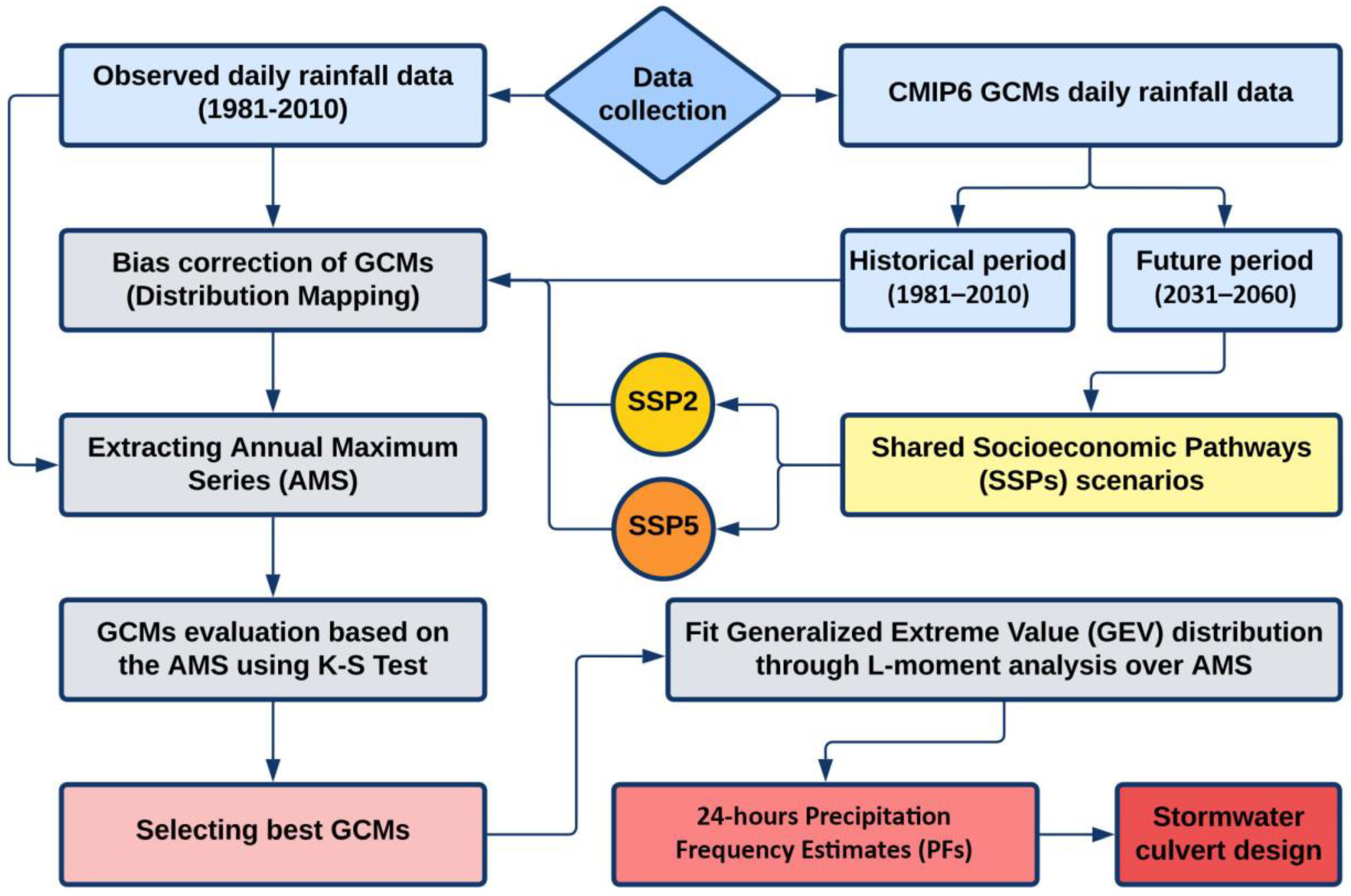
2. Materials and Methods
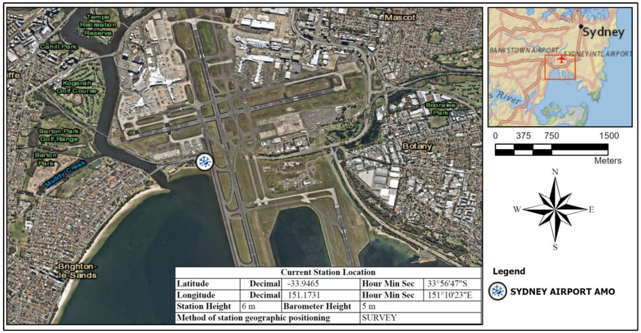
In the current study, we estimated the potential impact of climate change on rainfall extremes and designed stormwater infrastructure in Sydney, Australia. The framework used is outlined in Figure 1. The following subsections explain the data used and analysis performed.

2.1. Study Area

Sydney, located on Australia’s south-eastern coast, is the largest city in the country, with a population of approximately 5.4 million people [28]. It has an area of 12,367 square kilometres and is the capital of New South Wales [28]. The city is surrounded by various water bodies, including the Pacific Ocean and several bays and rivers. Sydney experiences a moderate oceanic climate with warm summers and mild winters. The city’s rainfall is relatively evenly distributed throughout the year, with a mean annual rainfall of approximately 1200 mm [29].
Sydney is an ideal case study to evaluate the impacts of climate change on stormwater management. The city’s location on the coast makes it susceptible to sea-level rise and storm surges, which can exacerbate flooding risks [30,31]. The city has experienced several significant floods, including the recent one in early July 2022. Heavy flooding broke out in the Central Coast and Sydney areas of New South Wales, Australia. Due to months of prior heavy rainfall, the land was already saturated, causing significant flood damage when additional rain fell. Some regions along the eastern seaboard experienced their third major flood of 2022. With the increasing frequency and intensity of extreme precipitation events due to climate change, the risk of flooding in Sydney is expected to increase [21].
Drainage infrastructure systems, such as culverts and stormwater drains, are essential in Sydney as they are designed to collect stormwater and control flooding. Hence, there is a need to refine the design of stormwater infrastructure systems to reduce the city’s vulnerability to flooding caused by climate change. To achieve this, we chose Sydney Airport AMO station as a showcase (Figure 2). This station has extensive and uninterrupted data records and is located in a strategic location in the city, making it an excellent representative of the broader Sydney region.

2.2. Data Overview

The long-term daily rainfall data spanning 30 years from 1981 to 2010 was obtained from the Bureau of methodology for Sydney Airport AMO station (http://bom.gov.au/climate/data/, accessed on 1 March 2023). Daily rainfall simulations from seven CMIP6 GCMs forced by the latest scenarios provided by the Intergovernmental Panel on Climate Change (IPCC) for both historical (1981–2010) and future (2031–2060) periods were downloaded from the Earth System Grid Federation (ESGF) website (https://esgf-node.llnl.gov/projects/cmip6/ (accessed on 1 March 2023)). The selected GCMs cover a range of different methodologies, parameterizations, and spatial resolutions, ensuring a diverse representation of the models commonly used in the field. This diversity adds robustness to our findings and provides a more comprehensive understanding of the role of GCMs in extreme event analysis. Our focus was not to utilize all available models, but rather to choose a representative subset that effectively highlights the importance of non-stationarity and the consideration of climate models. Table 1 provides further details on the specific models used in this study.
Table 1 provides the full names, abbreviations, providing institution name and ID, and spatial resolution of GCMs. Model abbreviations will be used hereafter to refer GCMs for brevity. The GCMs’ projections are reported under different scenarios of climate change. The IPCC has previously provided Representative Concentration Pathways (RCPs) as scenarios. However, these have been replaced by SSPs, which were developed to depict underlying socioeconomic characteristics and shared policy assumptions of that world for mitigating and adapting to climate change [32]. The five narratives outlined in the SSPs depict broad socioeconomic trends that could influence future societies and are designed to cover a wide range of potential futures.
We used the SSP2-4.5 (SSP2) and SSP5-8.5 (SSP5) scenarios to analyse climate change impacts on PFs and culvert design under two different limits of greenhouse gas emissions. SSP2, also known as the “middle-of-the-road” scenario, represents a moderate scenario that assumes future trends throughout the 21st century will follow historical patterns. The mitigation measures for decreasing greenhouse gas emissions are moderately implemented in SSP2, and one of the lowest CO2 levels compared to other scenarios is projected by the end of the century. On the other hand, SSP5 assumes high population and economic growth, along with a slower transition to low-emission technologies, leading to higher emissions. SSP5 is the worst-case scenario in terms of projecting the highest CO2 emissions by the end of this century [33,34]. By considering these scenarios in our analysis, we can better understand the potential consequences of different policy and development choices for the future of our planet.

2.3. Data Analysis

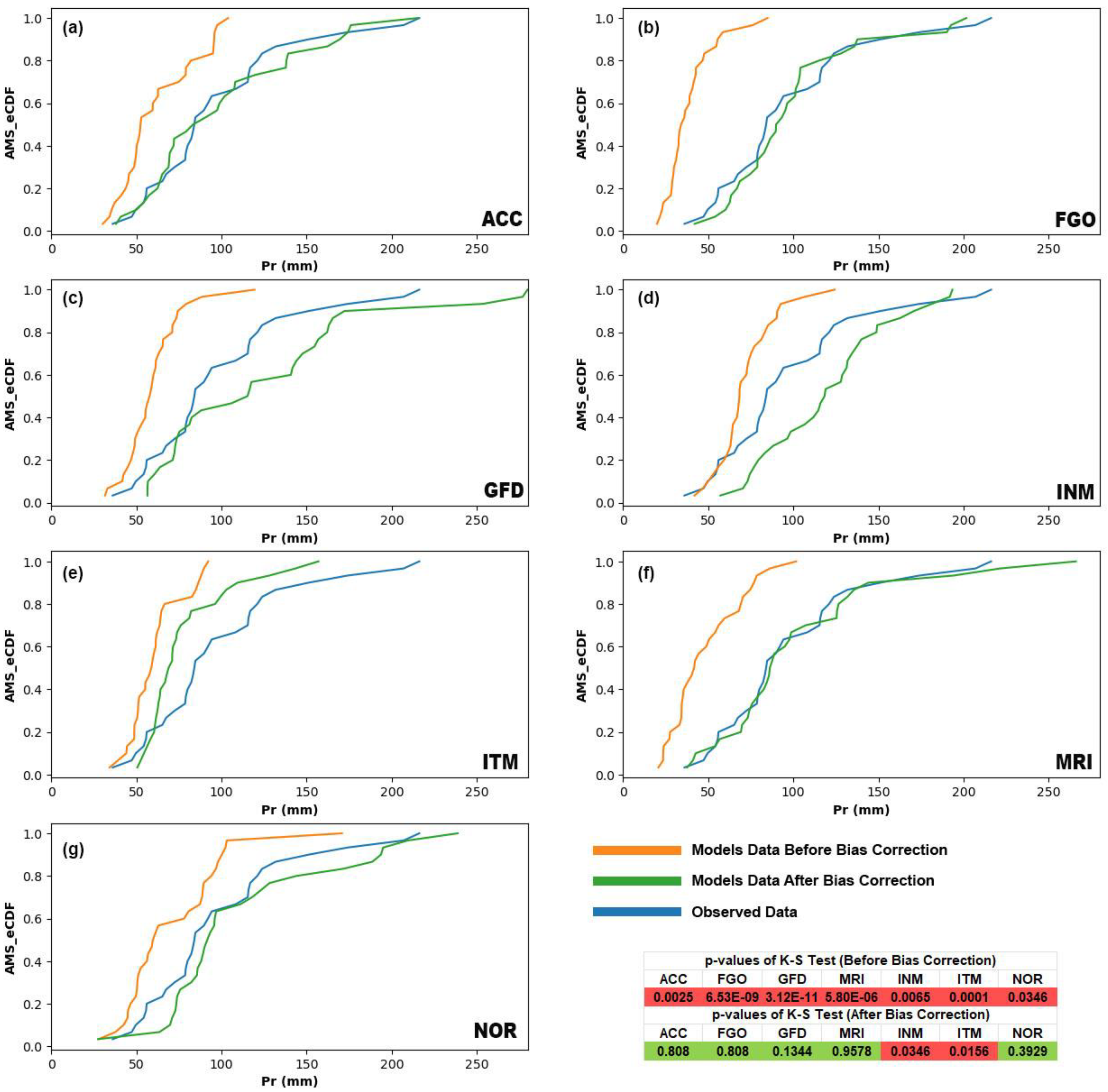
2.3.1. GCMs Bias Correction and Performance Evaluation

Recent research has utilized GCMs to investigate changes in high-impact weather events, such as extreme rainfall. However, GCMs typically are available at a spatial resolution of 100 km or more [35,36], which can introduce errors due to discretization and areal averaging within grid cells. As such, systematic model errors represent a primary source of bias in GCM data [37]. Statistical techniques, such as distribution mapping, can be used to correct the existing biases in model output and match observed values at a finer spatial resolution [38,39].
The selection of a bias correction algorithm has a substantial impact on the future projection of rainfall. Therefore, it is advisable to limit the choice of methods for current conditions to those that have demonstrated high performance in similar studies [40]. Distribution mapping is a well-known technique for correcting biases in stochastic variables such as rainfall. This approach corrects the biases present in GCM simulations by adjusting the distribution of the GCM data to match the observed distribution using transfer functions [37,41]. Unlike most methods that only correct the daily mean values, distribution mapping accounts for biases in all statistical moments [42]. CMhyd, a widely used statistical downscaling tool (https://swat.tamu.edu/software/cmhyd/ (accessed on 1 March 2023)), was used in this study to bias correct the GCM daily rainfall data [37,43].
While bias-corrected GCMs may agree on large-scale climate trends, there can be significant variations in their output at local scales [44]. This variation results in inherent uncertainty in the future projections of GCMs, making the process of decision-making challenging. Different GCMs can propose diverse adaptation strategies and corresponding plans that come with different implementation costs [4]. For example, variations in projected extreme events between GCMs can significantly affect the design size of stormwater drainage infrastructure, potentially doubling the cost [10]. Therefore, while evaluating multiple GCMs for a desired location is essential to broadly capture the characteristics of extreme events, there is a need to reduce the existing uncertainties in GCM outputs. Choosing the right model can further manage uncertainty, improve our method’s objectivity, and support more informed decisions [45,46].
Instead of selecting GCMs based on mean annual, seasonal, or monthly precipitation, extreme series were chosen to assess the impact of climate change on extreme events and design stormwater infrastructures in Sydney [4]. To generate the IDF curves and PFs, the extreme series is the main input; therefore, GCMs were selected based on their ability to reproduce the historical extreme series. It is expected that GCMs with higher performance in terms of extreme series in the historical period have more accountable projections [4]. The AMS, which involves selecting the maximum daily precipitation over the course of a year, was utilized as an extreme series to evaluate GCMs. This method is widely used for creating IDF curves and PFs [47], as recommended by the ARR guidelines [48]. The two-tailed Kolmogorov–Smirnov (K-S) test at the significant level of 0.05 [49] was used to evaluate the GCM’s performance in AMS. The empirical cumulative distribution function (eCDF) of observed AMS was compared against the eCDF of the bis-corrected GCMs’ AMS for the same historical period of 1981–2010. The null hypothesis in the K-S test is that the two samples (i.e., observed AMS and GCM AMS) have the same underlying distribution. The p-value represents the probability of not rejecting the null hypothesis, which is calculated based on the maximum difference between the CDFs (i.e., eCDFs in this case) of the two samples. A high p-value (i.e., >0.05) suggests that the differences between the two samples are likely due to random sampling error and there is not enough evidence to reject the null hypothesis that both samples are from the same distribution. In contrast, a low p-value rejects the null hypothesis and indicates that the differences may be due to the samples having different underlying distributions [10]. This test shows whether the given bias-corrected GCM provides nearly the same AMS as the observed data, which is a metric for selecting GCMs for generating IDF curves [50].
The ensemble of selected GCMs (α = 0.05) was used to further manage uncertainty and increase confidence in climate projections by generating a range of different possible outcomes. Ensemble modelling helps to account for the fact that no single GCM is perfect and provides insight into the range of potential future climates. Each GCM has its strengths and weaknesses, and by combining the outputs of multiple selected models, we can leverage the strengths of each model while mitigating its weaknesses. This can lead to more robust and reliable projections of future climate change [51,52,53].

2.3.2. Extreme Value Fitting

This section presents a summary of the process used to derive the 24 h PFs for annual exceedance probabilities (AEPs) ranging from 50% to 1%, which are used for generating IDF curves appropriate for most design situations [48]. The AEP of 50% to 1% corresponds to 2 yr to 100 yr rainfall events. PFs were generated in this study using the ARR guidelines, which is the primary source for engineering design in Australia. [48]. This involves several steps, including collating quality-controlled rainfall data, extraction of extreme value series, and frequency analysis.
The AMS was used instead of PDS to define the extreme value series due to its unambiguous definition, relatively simple application, and the problem of bias associated with the PDS for less frequent AEPs [48]. Daily AMS was converted to 24 h AMS using a conversion factor of 1.15, provided by ARR guidelines, to convert daily rainfall observation restricted to 9:00 a.m. to 9:00 a.m. to the actual, unrestricted 24 h events. The generalised extreme value (GEV) distribution was used to fit the AMS, which best fits the AMS on an at-site analysis per ARR guidelines [48]. L-moment, a widely used method in rainfall and flood frequency analysis was used to fit AMS to GEV using a linear combination of the mean, variation, and skewness of data, known as L-moments [54]. L-moment is an efficient method for fitting the data and does not have biases in sample estimates, particularly in higher-order moments, unlike ordinary moments [55]. We utilized the lmomRFA package in R 4.3.0 to implement the L-moments for fitting GEV and generating 24 h design PFs with return periods of 100, 50, 25, 10, 5, and 2 years [56,57].

2.3.3. Illustrative Culvert Design Example

A culvert design example was chosen to demonstrate how the projected change in design rainfall may affect stormwater drainage infrastructure design in Sydney. The example was demonstrated using the selected GCMs and their ensemble. The design example for the culvert was performed on a hypothetical watershed that was relatively urbanized, with an area of 4 hectares (i.e., 1 acre) and a runoff coefficient of 0.65. It was carried out for the 1 h 100 yr event at the Sydney airport station using baseline PFs of ARR and predicted PFs from the GCMs for two scenarios (i.e., SSP2, SSP5) [4,10]. The ratio of the 1 h to 24 h 100 yr historical ARR PF was obtained at Sydney airport station. This ratio was multiplied by the 24 h 100 yr projected PFs from the GCMs to obtain a 1 h projected event for the culvert design. To calculate peak stormflow for design, the rational method was used, as shown in Equation (1). In this equation, Q represents the peak stormflow (m3/s), which is calculated using the runoff coefficient (C), the average rainfall intensity (I) for a given duration and return period, and the area (A) of the watershed. The design was carried out for an average rainfall intensity with a duration of 1 h, assuming a time of concentration of 1 h for the small watershed [10,58].
Q = C I A
Manning’s equation (Equation (2)) was used to determine the appropriate size for the stormwater culvert. The equation uses Rh as the hydraulic radius (m), S0 (m/m) as the culvert slope, and n as the Manning roughness coefficient. In this particular case, a circular concrete culvert was designed using Manning’s equation with a culvert slope of 0.005 and a Manning roughness coefficient of 0.013 [59].
Q = 1 n A R h 2 / 3 S 0 1 / 2
The computed diameters of the culvert for both the past and projected extreme precipitation events were approximated to the closest standard pipe size used in Australia, which includes sizes of 600, 675, 750, and 825 mm.

3. Results and Discussion

3.1. Evaluation of GCMs Performance

The ability of bias-corrected GCMs to replicate the AMS during the historical period (1981–2010) was tested using the K-S test (α = 0.05). AMS is the primary input for calculating PFs, and therefore, it was crucial to evaluate the GCMs’ skill in replicating AMS accurately. Figure 3 shows the eCDFs of AMS for the observed, raw GCMs and bias-corrected GCMs, along with the associated K-S p-values in the historical period. The findings indicated that the distribution mapping bias-correction method significantly improves the fitting of all GCMs to the observed data. This is shown by shifting the raw AMS eCDF of models toward the observed AMS eCDF using bias correction. Some models (e.g., MRI, see Figure 3f) show a very similar AMS eCDF to the observed AMS after bias-correcting compared to the raw AMS eCDF. Further, the K-S test results confirm the importance of bias correction, with all models showing increased p-values after bias correction. However, two models (i.e., ITM, see Figure 3e; INM, see Figure 3d) reject the K-S test null hypothesis, indicating that bias-correcting could not improve (i.e., p-value < α = 0.05) the performance of these GCMs enough to produce similar AMS to the observed AMS in the historical period. Therefore, five out of seven bias-corrected GCMs (i.e., ACC, see Figure 3a; FGO, see Figure 3b; GFD, see Figure 3c; MRI, see Figure 3f; NOR, see Figure 3g) passed the K-S test and were selected for the rest of the analysis. These models demonstrated higher performance for generating extreme events in the study area. The ensemble of the selected GCMs was used to further reduce uncertainty, increase confidence in projections, and account for the strengths and weaknesses of different models. To encompass all potential future projections based on the chosen GCMs, culvert design practices and projected 24 h PFs are presented for each individual GCM as well as the ensemble of selected models. The findings demonstrate the effectiveness of the distribution mapping approach in correcting biases and emphasize the significance of selecting appropriate models to precisely project extreme events.

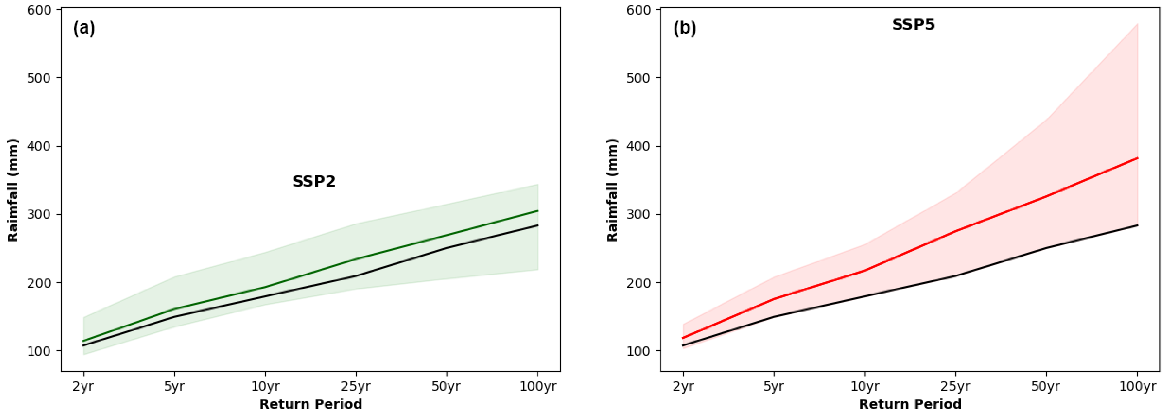
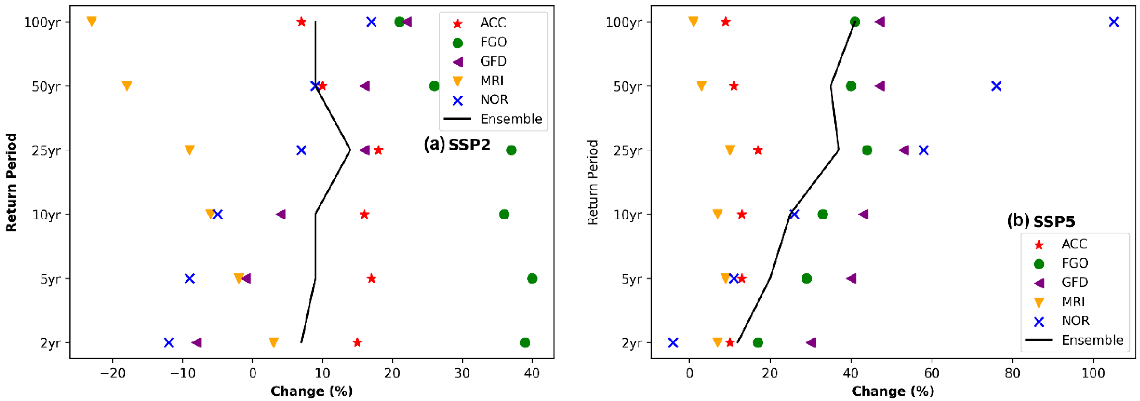
3.2. Projected 24 h Precipitation Frequency Estimates

Figure 4 depicts the 24 h PFs for five return periods (i.e., 2 yr, 5 yr, 10 yr, 25 yr, 50 yr, 100 yr) and two scenarios (i.e., SSP5, see Figure 4b and SSP2, see Figure 3a) for the Sydney airport station, based on the historical and projected data. The historical PFs were obtained from the ARR design rainfall data [48]. The projected PFs were estimated using the selected GCMs and their ensemble for two scenarios: SSP5 and SSP2. Figure 5 shows the changes in the projected 24 h PFs relative to historical values of the ARR for the selected GCMs and their ensemble for all return periods under the two scenarios in SSP5 (see Figure 5b) and SSP2 (see Figure 5a). The results (see Figure 4 and Figure 5) highlight that projected extreme rainfall events are expected to occur at bigger magnitudes than in the historical period, consistent with previous studies [2,10,60,61]. For both scenarios, the historical PFs lie between the lowest projected PFs and the ensemble of GCMs (see Figure 4). This shows a consistent underestimation of historical PFs compared to the average projected PFs shown by the GCMs ensemble (see Figure 4). This is sounder for the worst-case scenario in SSP5 (see Figure 4b), where historical PFs lie almost at the lowest limit of projected PFs. The projected 24 h 100yr PFs for the ensemble of models are 308 mm and 398 mm for SSP2 (see Figure 4a) and SSP5 (see Figure 4b), respectively. These are, respectively, 9% (see Figure 5a) and 41% higher (see Figure 5b) compared to the historical value of ARR (i.e., 283 mm) for the same event.
The divergence between the projected PFs and historical values increases with longer return periods, regardless of the future scenario or GCM used, which aligns with earlier findings [60,62]. For extreme events, this shows the underestimation of historical PFs is even higher. Figure 4 and Figure 5 show how almost consistently, for both scenarios, the increase in the ensemble of projected PFs compared to the historical PFs rises for the more extreme events. Uncertainties in the projected PFs also increase for more extreme events compared to less extreme events for both scenarios and most models (Figure 4 and Figure 5). For example, for SSP5, the range for the projected 24 h 2 yr PFs is 36 mm (from 103 mm to 139 mm), while the same range for 24 h 100 yr is 293 mm (from 286 mm to 579 mm) (see Figure 4b).
As expected, the projected PFs are generally higher for the worst-case scenario in SSP5 compared to SSP2. SSP2 assumes that future trends will follow the historical trends with less projected greenhouse gas emissions compared to SSP5, with the highest projected emission that results in more intense projected precipitation. The average increase in projected PFs based on the models’ ensemble for all return periods is 9% and 28% for SSP2 (see Figure 5a) and SSP5 (see Figure 5b), respectively. On the other hand, the uncertainty is also higher for SSP5 (see Figure 4b) compared to SSP2 (see Figure 4a), with a larger range of projected PFs. The average range of 24 h PFs in all events (i.e., 2 yr, 5 yr, 10 yr, 25 yr, 50 yr, 100 yr) for the selected models is 89 mm and 120 mm for SSP5 and SSP2, respectively.
These findings suggest that climate change may lead to more severe rainfall extremes, particularly under the SSP5 scenario, which warrants proactive measures to mitigate potential impacts. The projected PFs suggest that the risk of extreme events in the future may be underestimated by the currently used stationary approach of ARR. Infrastructure such as stormwater drainage systems, roads, and bridges, which are designed based on stationary assumptions, possibly will not have the capacity to withstand the expected extreme events resulting from climate change over their expected service life.

3.3. Culvert Design under Climate Change

A typical culvert was chosen as a representative case study to demonstrate the impact of climate change on infrastructure. Table 2 displays the rainfall intensities of 1 h 100 yr events and the estimated peak stormflows for two scenarios of the models’ ensemble, in addition to the historical values of ARR. The results in Table 2 indicate that peak stormflows are expected to increase by 8% and 41% for the SSP2 and SSP5 scenarios, respectively, compared to the past values calculated using ARR data. These findings suggest that culverts currently designed based on ARR may not be sufficient in the future for both scenarios.
Figure 6 depicts the complete range of differences in culvert design sizes across various models and scenarios due to climate change at Sydney airport station. The design was evaluated against historical values obtained from ARR, which represent the main foundation for engineering design in the study region.
According to the past values of ARR, a culvert with the size of 675 mm is adequate to manage a 1 h 100 yr storm in the Sydney study area. The designed culvert size under climate change varies depending on the scenario, ranging from 600 mm to 825 mm. However, with the projected increase in extreme weather events, larger culverts are required to handle the same event in the future under the worst-case scenario. The ensemble of GCMs for SSP5 suggests one size higher culvert of 750 mm for 2031–2060. The ensemble of GCMs for SSP2 suggests the same culvert size (i.e., 675 mm) as the past value of ARR; the same results were also obtained by Ghasemi Tousi et al. (2021) [4] for the best-selected model of MPI-ESM1- 2-H in a case study in Tucson, AZ, U.S.
The selection of GCMs can impact the results obtained. Different models may utilize distinct assumptions and numerical schemes, leading to different projections [63,64]. Nonetheless, the sensitivity of results to GCM selection is a subject of ongoing research and debate. It is crucial to recognize these limitations and uncertainties to properly interpret and apply the findings of GCMs in climate-related research and decision-making processes. Furthermore, other factors, such as land use change and topography, can significantly impact rainfall patterns [65,66,67,68]. Land use changes, such as urbanization, deforestation, and agricultural practices, can alter the surface characteristics of an area. Consequently, these changes can disrupt natural hydrological cycles, affect evapotranspiration rates, and change the distribution and intensity of rainfall [66,67]. Similarly, topography plays a vital role in shaping rainfall patterns. The presence of topographic features can influence the movement and intensity of weather systems, leading to localized variations in rainfall [65,69]. In our study, we focused specifically on quantifying the impacts of climate change on extreme rainfall events. Therefore, we did not consider other factors, such as land use change or topography, which could affect rainfall patterns. Future research should examine the combined impacts of climate change, land use change, and topography on extreme rainfall events. By integrating these multiple dimensions, researchers can better understand the complexities of future implications of extreme rainfall events.

4. Conclusions

In conclusion, incorporating non-stationary PFs in infrastructure design flood mitigation is essential for building resilience in a changing climate, particularly in urban areas such as Sydney. In recent years, the City of Sydney has experienced several extreme weather events, including floods, and climate models predict that such events will likely increase [70,71]. As climate change continues to exacerbate extreme weather events, it is crucial to use a forward-looking approach to flood estimation that accounts for non-stationary factors such as changing rainfall patterns and intensifying rainfall events. This study highlights the importance of model selection in generating PFs and IDF curves, where out of seven climate models, only five of them were selected, and their ensemble was used to represent the projected extreme events at Sydney airport. The projected 24 h 100 yr rainfall events are increased by 9% to 41% for the least and worst-case scenario in 2031–2060. The historical PFs from ARR are consistently underestimating the future rainfall events, particularly the more extreme events under the horizon of 2031–2060 in Sydney. The projected PFs from this study and historical PFs from ARR were used in a typical culvert design in Sydney to showcase the impact of climate change. For the worst-case scenario (i.e., SSP5), based on the 2031–2060 projected 1 h 100 yr event, the required culvert is one size higher (i.e., 750 mm) than the culvert size (i.e., 675 mm) needed for the same storm based on historical values of ARR and the less extreme scenario (i.e., SSP2). This is valuable information that can be used by Sydney planners and officials to practically incorporate the impact of climate change in their policies regarding flood mitigation and resilient infrastructure design in Sydney. The same framework can also be used by other case studies seeking more resilient policies coping with climate change. The findings of this research can inform policy decisions and guide the development of more sustainable and resilient communities that are better equipped to cope with the challenges of a changing climate.

Author Contributions

Conceptualization, S.D., E.T., S.A., and A.S.; methodology, S.D., E.T, S.A.; software, S.D., E.T., A.S.; validation, S.D. and E.T.; formal analysis, S.D.; investigation, S.D. and S.A.; resources, S.D.; data curation, S.D.; writing—original draft preparation, S.D.; writing—review and editing, S.D., E.T., A.S., and S.A.; visualization, A.S.; supervision, S.A.; project administration, S.A.. All authors have read and agreed to the published version of the manuscript.

Funding

This research received no external funding.

Data Availability Statement

The data that support the findings of this study are available upon request. Requests for access to the data should be addressed to Shahab Doulabian at [email protected].

Conflicts of Interest

The authors declare no conflict of interest.

References

  1. Abram, N.J.; Henley, B.J.; Gupta, A.S.; Lippmann, T.J.R.; Clarke, H.; Dowdy, A.J.; Sharples, J.J.; Nolan, R.H.; Zhang, T.; Wooster, M.J.; et al. Connections of climate change and variability to large and extreme forest fires in southeast Australia. Commun. Earth Environ. 2021, 2, 8. [Google Scholar] [CrossRef]
  2. Lopez-Cantu, T.; Prein, A.F.; Samaras, C. Uncertainties in Future U.S. Extreme Precipitation From Downscaled Climate Projections. Geophys. Res. Lett. 2020, 47, e2019GL086797. [Google Scholar] [CrossRef]
  3. Pour, S.H.; Abd Wahab, A.K.; Shahid, S.; Asaduzzaman, M.; Dewan, A. Low impact development techniques to mitigate the impacts of climate-change-induced urban floods: Current trends, issues and challenges. Sustain. Cities Soc. 2020, 62, 102373. [Google Scholar] [CrossRef]
  4. Tousi, E.G.; O’brien, W.; Doulabian, S.; Toosi, A.S. Climate changes impact on stormwater infrastructure design in Tucson Arizona. Sustain. Cities Soc. 2021, 72, 103014. [Google Scholar] [CrossRef]
  5. Haghighatafshar, S.; Becker, P.; Moddemeyer, S.; Persson, A.; Sörensen, J.; Aspegren, H.; Jönsson, K. Paradigm shift in engineering of pluvial floods: From historical recurrence intervals to risk-based design for an uncertain future. Sustain. Cities Soc. 2020, 61, 102317. [Google Scholar] [CrossRef]
  6. Cea, L.; Costabile, P. Flood Risk in Urban Areas: Modelling, Management and Adaptation to Climate Change. A Review. Hydrology 2022, 9, 50. [Google Scholar] [CrossRef]
  7. Silva, M.M.; Costa, J.P. Urban Floods and Climate Change Adaptation: The Potential of Public Space Design When Accommodating Natural Processes. Water 2018, 10, 180. [Google Scholar] [CrossRef]
  8. Yan, L.; Xiong, L.; Jiang, C.; Zhang, M.; Wang, D.; Xu, C. Updating intensity–duration–frequency curves for urban infrastructure design under a changing environment. Wiley Interdiscip. Rev. Water 2021, 8, e1519. [Google Scholar] [CrossRef]
  9. Kourtis, I.M.; Tsihrintzis, V.A. Update of intensity-duration-frequency (IDF) curves under climate change: A review. Water Supply 2022, 22, 4951–4974. [Google Scholar] [CrossRef]
  10. Cook, L.M.; McGinnis, S.; Samaras, C. The effect of modeling choices on updating intensity-duration-frequency curves and stormwater infrastructure designs for climate change. Clim. Chang. 2020, 159, 289–308. [Google Scholar] [CrossRef]
  11. Kourtis, I.M.; Nalbantis, I.; Tsakiris, G.; Psiloglou, B.; Tsihrintzis, V.A. Updating IDF Curves Under Climate Change: Impact on Rainfall-Induced Runoff in Urban Basins. Water Resour. Manag. 2022, 37, 2403–2428. [Google Scholar] [CrossRef]
  12. Ren, H.; Hou, Z.J.; Wigmosta, M.; Liu, Y.; Leung, L.R. Impacts of Spatial Heterogeneity and Temporal Non-Stationarity on Intensity-Duration-Frequency Estimates—A Case Study in a Mountainous California-Nevada Watershed. Water 2019, 11, 1296. [Google Scholar] [CrossRef]
  13. Ragno, E.; AghaKouchak, A.; Love, C.A.; Cheng, L.; Vahedifard, F.; Lima, C.H. Quantifying changes in future intensity-duration-frequency curves using multimodel ensemble simulations. Water Resour. Res. 2018, 54, 1751–1764. [Google Scholar] [CrossRef]
  14. Agilan, V.; Umamahesh, N. Is the covariate based non-stationary rainfall IDF curve capable of encompassing future rainfall changes? J. Hydrol. 2016, 541, 1441–1455. [Google Scholar] [CrossRef]
  15. Li, J.; Johnson, F.; Evans, J.; Sharma, A. A comparison of methods to estimate future sub-daily design rainfall. Adv. Water Resour. 2017, 110, 215–227. [Google Scholar] [CrossRef]
  16. King, A.D.; Pitman, A.J.; Henley, B.J.; Ukkola, A.M.; Brown, J.R. The role of climate variability in Australian drought. Nat. Clim. Chang. 2020, 10, 177–179. [Google Scholar] [CrossRef]
  17. Nicholls, N.; Drosdowsky, W.; Lavery, B. Australian rainfall variability and change. Weather 1997, 52, 66–72. [Google Scholar] [CrossRef]
  18. Freund, M.; Henley, B.J.; Karoly, D.J.; Allen, K.J.; Baker, P.J. Multi-century cool- and warm-season rainfall reconstructions for Australia’s major climatic regions. Clim. Past 2017, 13, 1751–1770. [Google Scholar] [CrossRef]
  19. Phillips, N.; Nogrady, B. The race to decipher how climate change influenced Australia’s record fires. Nature 2020, 577, 610–612. [Google Scholar] [CrossRef]
  20. Vardoulakis, S.; Matthews, V.; Bailie, R.S.; Hu, W.; Salvador-Carulla, L.; Barratt, A.L.; Chu, C. Building resilience to Australian flood disasters in the face of climate change. Med. J. Aust. 2022, 217, 342–345. [Google Scholar] [CrossRef]
  21. El-Zein, A.; Ahmed, T.; Tonmoy, F. Geophysical and social vulnerability to floods at municipal scale under climate change: The case of an inner-city suburb of Sydney. Ecol. Indic. 2020, 121, 106988. [Google Scholar] [CrossRef]
  22. Hallegatte, S.; Green, C.; Nicholls, R.J.; Corfee-Morlot, J. Future flood losses in major coastal cities. Nat. Clim. Chang. 2013, 3, 802–806. [Google Scholar] [CrossRef]
  23. Axelsson, C.; Soriani, S.; Culligan, P.; Marcotullio, P. Urban policy adaptation toward managing increasing pluvial flooding events under climate change. J. Environ. Plan. Manag. 2020, 64, 1408–1427. [Google Scholar] [CrossRef]
  24. Kc, S.; Shrestha, S.; Ninsawat, S.; Chonwattana, S. Predicting flood events in Kathmandu Metropolitan City under climate change and urbanisation. J. Environ. Manag. 2021, 281, 111894. [Google Scholar] [CrossRef] [PubMed]
  25. Veiga, M.M.; Castiglia-Feitosa, R.; Marques, R.C. Analyzing barriers for stormwater management utilities. Water Supply 2021, 21, 1506–1513. [Google Scholar] [CrossRef]
  26. Mishra, B.K.; Chakraborty, S.; Kumar, P.; Saraswat, C. Urban stormwater management: Practices and governance. In Sustainable Solutions for Urban Water Security; Water Science and Technology Library; Springer: Cham, Switzerland, 2020; Volume 93, pp. 115–146. [Google Scholar] [CrossRef]
  27. Teshome, M. A Review of Recent Studies on Urban Stormwater Drainage System for Urban Flood Management. Architecture 2020, 2020100295. [Google Scholar] [CrossRef]
  28. Statistics, A.B.O. Census Community Profiles. 2011. Census of Population and Housing. Available online: https://www.abs.gov.au/ (accessed on 1 March 2023).
  29. Pilgrim, D.H.; Cordery, I. Rainfall Temporal Patterns for Design Floods. J. Hydraul. Div. 1975, 101, 81–95. [Google Scholar] [CrossRef]
  30. Hague, B.S.; McGregor, S.; Murphy, B.F.; Reef, R.; Jones, D.A. Sea Level Rise Driving Increasingly Predictable Coastal Inundation in Sydney, Australia. Earth’s Future 2020, 8, e2020EF001607. [Google Scholar] [CrossRef]
  31. Dall’Osso, F.; Dominey-Howes, D.; Moore, C.; Summerhayes, S.; Withycombe, G. The exposure of Sydney (Australia) to earthquake-generated tsunamis, storms and sea level rise: A probabilistic multi-hazard approach. Sci. Rep. 2014, 4, 7401. [Google Scholar] [CrossRef]
  32. O’Neill, B.C.; Tebaldi, C.; van Vuuren, D.P.; Eyring, V.; Friedlingstein, P.; Hurtt, G.; Knutti, R.; Kriegler, E.; Lamarque, J.-F.; Lowe, J.; et al. The Scenario Model Intercomparison Project (ScenarioMIP) for CMIP6. Geosci. Model Dev. 2016, 9, 3461–3482. [Google Scholar] [CrossRef]
  33. Pörtner, H.O.; Roberts, D.C.; Poloczanska, E.S.; Mintenbeck, K.; Tignor, M.; Alegría, A.; Craig, M.; Langsdorf, S.; Löschke, S.; Möller, V.; et al. Summary for policymakers. In Climate Change 2022: Impacts, Adaptation, and Vulnerability: Contribution of Working Group II to the Sixth Assessment Report of the Intergovernmental Panel on Climate Change; IPCC: Cambridge, UK; New York, NY, USA, 2022; pp. 3–33. [Google Scholar]
  34. Riahi, K.; Van Vuuren, D.P.; Kriegler, E.; Edmonds, J.; O’Neill, B.C.; Fujimori, S.; Bauer, N.; Calvin, K.; Dellink, R.; Fricko, O.; et al. The Shared Socioeconomic Pathways and their energy, land use, and greenhouse gas emissions implications: An overview. Glob. Environ. Chang. 2017, 42, 153–168. [Google Scholar] [CrossRef]
  35. Wilby, R.; Wigley, T. Downscaling general circulation model output: A review of methods and limitations. Prog. Phys. Geogr. Earth Environ. 1997, 21, 530–548. [Google Scholar] [CrossRef]
  36. Wilby, R.L.; Charles, S.P.; Zorita, E.; Timbal, B.; Whetton, P.; Mearns, L.O. Guidelines for Use of Climate Scenarios Developed from Statistical Downscaling Methods. Analysis 2004, 27, 1–27. [Google Scholar]
  37. Teutschbein, C.; Seibert, J. Bias correction of regional climate model simulations for hydrological climate-change impact studies: Review and evaluation of different methods. J. Hydrol. 2012, 456–457, 12–29. [Google Scholar] [CrossRef]
  38. Yang, Y.; Bai, L.; Wang, B.; Wu, J.; Fu, S. Reliability of the global climate models during 1961–1999 in arid and semiarid regions of China. Sci. Total Environ. 2019, 667, 271–286. [Google Scholar] [CrossRef]
  39. Christensen, J.H.; Boberg, F.; Christensen, O.B.; Lucas-Picher, P. On the need for bias correction of regional climate change projections of temperature and precipitation. Geophys. Res. Lett. 2008, 35, L20709. [Google Scholar] [CrossRef]
  40. Toosi, A.S.; Danesh, S.; Tousi, E.G.; Doulabian, S. Annual and seasonal reliability of urban rainwater harvesting system under climate change. Sustain. Cities Soc. 2020, 63, 102427. [Google Scholar] [CrossRef]
  41. Gutowski Jr, W.J.; Decker, S.G.; Donavon, R.A.; Pan, Z.; Arritt, R.W.; Takle, E.S. Temporal–spatial scales of observed and simulated precipitation in central US climate. J. Clim. 2003, 16, 3841–3847. [Google Scholar] [CrossRef]
  42. Switanek, M.B.; Troch, P.A.; Castro, C.L.; Leuprecht, A.; Chang, H.-I.; Mukherjee, R.; Demaria, E.M.C. Scaled distribution mapping: A bias correction method that preserves raw climate model projected changes. Hydrol. Earth Syst. Sci. 2017, 21, 2649–2666. [Google Scholar] [CrossRef]
  43. Teutschbein, C.; Seibert, J. Regional Climate Models for Hydrological Impact Studies at the Catchment Scale: A Review of Recent Modeling Strategies. Geogr. Compass 2010, 4, 834–860. [Google Scholar] [CrossRef]
  44. Zappa, G.; Shepherd, T.G. Storylines of Atmospheric Circulation Change for European Regional Climate Impact Assessment. J. Clim. 2017, 30, 6561–6577. [Google Scholar] [CrossRef]
  45. McSweeney, C.F.; Jones, R.G.; Lee, R.W.; Rowell, D.P. Selecting CMIP5 GCMs for downscaling over multiple regions. Clim. Dyn. 2015, 44, 3237–3260. [Google Scholar] [CrossRef]
  46. Shepherd, T.G.; Boyd, E.; Calel, R.A.; Chapman, S.C.; Dessai, S.; Dima-West, I.M.; Fowler, H.J.; James, R.; Maraun, D.; Martius, O.; et al. Storylines: An alternative approach to representing uncertainty in physical aspects of climate change. Clim. Chang. 2018, 151, 555–571. [Google Scholar] [CrossRef] [PubMed]
  47. Vrban, S.; Wang, Y.; McBean, E.A.; Binns, A.; Gharabaghi, B. Evaluation of Stormwater Infrastructure Design Storms Developed Using Partial Duration and Annual Maximum Series Models. J. Hydrol. Eng. 2018, 23, 04018051. [Google Scholar] [CrossRef]
  48. Ball, J.; Babister, M.; Nathan, R.; Weeks, W.; Weinmann, E.; Retallick, M.; Testoni, I. (Eds.) Australian Rainfall and Runoff: A Guide to Flood Estimation; Commonwealth of Australia: Canberra, Australia, 2016. [Google Scholar]
  49. Massey, F.J., Jr. The Kolmogorov-Smirnov Test for Goodness of Fit. J. Am. Stat. Assoc. 1951, 46, 68–78. [Google Scholar] [CrossRef]
  50. Motamarri, S.; Boccelli, D.L. Development of a neural-based forecasting tool to classify recreational water quality using fecal indicator organisms. Water Res. 2012, 46, 4508–4520. [Google Scholar] [CrossRef]
  51. Pfeifer, S.; Bülow, K.; Gobiet, A.; Hänsler, A.; Mudelsee, M.; Otto, J.; Rechid, D.; Teichmann, C.; Jacob, D. Robustness of Ensemble Climate Projections Analyzed with Climate Signal Maps: Seasonal and Extreme Precipitation for Germany. Atmosphere 2015, 6, 677–698. [Google Scholar] [CrossRef]
  52. Jose, D.M.; Vincent, A.M.; Dwarakish, G.S. Improving multiple model ensemble predictions of daily precipitation and temperature through machine learning techniques. Sci. Rep. 2022, 12, 4678. [Google Scholar] [CrossRef]
  53. Semenov, M.; Stratonovitch, P. Use of multi-model ensembles from global climate models for assessment of climate change impacts. Clim. Res. 2010, 41, 1–14. [Google Scholar] [CrossRef]
  54. Hosking, J.R.M.; Wallis, J.R. Regional Frequency Analysis: An Approach Based on L-Moments; Cambridge University Press: Cambridge, UK, 1997. [Google Scholar] [CrossRef]
  55. Hosking, J.R. L-moments: Analysis and estimation of distributions using linear combinations of order statistics. J. R. Stat. Soc. Ser. B Methodol. 1990, 52, 105–124. [Google Scholar] [CrossRef]
  56. Hosking, J. Regional Frequency Analysis Using L-Moments, lmomRFA R Package, Version 2.2. 2009. Available online: https://cran.r-project.org/web/packages/lmomRFA/index.html (accessed on 10 March 2023).
  57. Team, R.C. R: A Language and Environment for Statistical Computing; R Foundation for Statistical Computing: Vienna, Austria, 2016; Available online: http://www.R-project.org/ (accessed on 15 March 2023).
  58. McCuen, R.H. Hydrologic Analysis and Design; Pearson Prentice Hall Upper: Saddle River, NJ, USA, 2005; Volume 3. [Google Scholar]
  59. Normann, J.M.; Houghtalen, R.J.; Johnston, W.J. Hydraulic Design of Highway Culverts. HDS-5 (Hydraulic Design Series 5). FHWA-IP-85-15; NTIS Publication PB86196961: Alexandria, VA, USA, 1985. [Google Scholar]
  60. Coulibaly, P.; Shi, X. Identification of the Effect of Climate Change on Future Design Standards of Drainage Infrastructure in Ontario; McMaster University: Hamilton, ON, USA, 2005; p. 82. [Google Scholar]
  61. Schardong, A.; Simonovic, S.P.; Gaur, A.; Sandink, D. Web-Based Tool for the Development of Intensity Duration Frequency Curves under Changing Climate at Gauged and Ungauged Locations. Water 2020, 12, 1243. [Google Scholar] [CrossRef]
  62. Fadhel, S.; Rico-Ramirez, M.A.; Han, D. Uncertainty of Intensity–Duration–Frequency (IDF) curves due to varied climate baseline periods. J. Hydrol. 2017, 547, 600–612. [Google Scholar] [CrossRef]
  63. Kaini, S.; Nepal, S.; Pradhananga, S.; Gardner, T.; Sharma, A.K. Representative general circulation models selection and downscaling of climate data for the transboundary Koshi river basin in China and Nepal. Int. J. Clim. 2019, 40, 4131–4149. [Google Scholar] [CrossRef]
  64. Her, Y.; Yoo, S.-H.; Cho, J.; Hwang, S.; Jeong, J.; Seong, C. Uncertainty in hydrological analysis of climate change: Multi-parameter vs. multi-GCM ensemble predictions. Sci. Rep. 2019, 9, 4974. [Google Scholar] [CrossRef]
  65. Li, S.; Yang, S.; Ran, L. Impacts of changes in land cover and topography on a heavy precipitation event in Central Asia. Atmos. Ocean. Sci. Lett. 2022, 15, 100207. [Google Scholar] [CrossRef]
  66. Kayitesi, N.M.; Guzha, A.C.; Mariethoz, G. Impacts of land use land cover change and climate change on river hydro-morphology- a review of research studies in tropical regions. J. Hydrol. 2022, 615, 128702. [Google Scholar] [CrossRef]
  67. Wierik, S.A.T.; Cammeraat, E.L.H.; Gupta, J.; Artzy-Randrup, Y.A. Reviewing the Impact of Land Use and Land-Use Change on Moisture Recycling and Precipitation Patterns. Water Resour. Res. 2021, 57, e2020WR029234. [Google Scholar] [CrossRef]
  68. Winkler, K.; Fuchs, R.; Rounsevell, M.; Herold, M. Global land use changes are four times greater than previously estimated. Nat. Commun. 2021, 12, 2501. [Google Scholar] [CrossRef]
  69. Anders, A.M.; Roe, G.H.; Hallet, B.; Montgomery, D.R.; Finnegan, N.J.; Putkonen, J. Spatial patterns of precipitation and topography in the Himalaya. In Tectonics, Climate, and Landscape Evolution; Geological Society of America: Boulder, CO, USA, 2006. [Google Scholar] [CrossRef]
  70. Rice, M.; Hughes, L.; Steffen, W.; Bradshaw, S.; Bambrick, H.; Hutley, N.; Morgan, W. A Supercharged Climate: Rain Bombs, Flash Flooding and Destruction; Climate Council: New South Wales, Australia, 2022. [Google Scholar]
  71. Hague, B.S.; Jones, D.A.; Jakob, D.; McGregor, S.; Reef, R. Australian coastal flooding trends and forcing factors. Earth’s Future 2022, 10, e2021EF002483. [Google Scholar] [CrossRef]
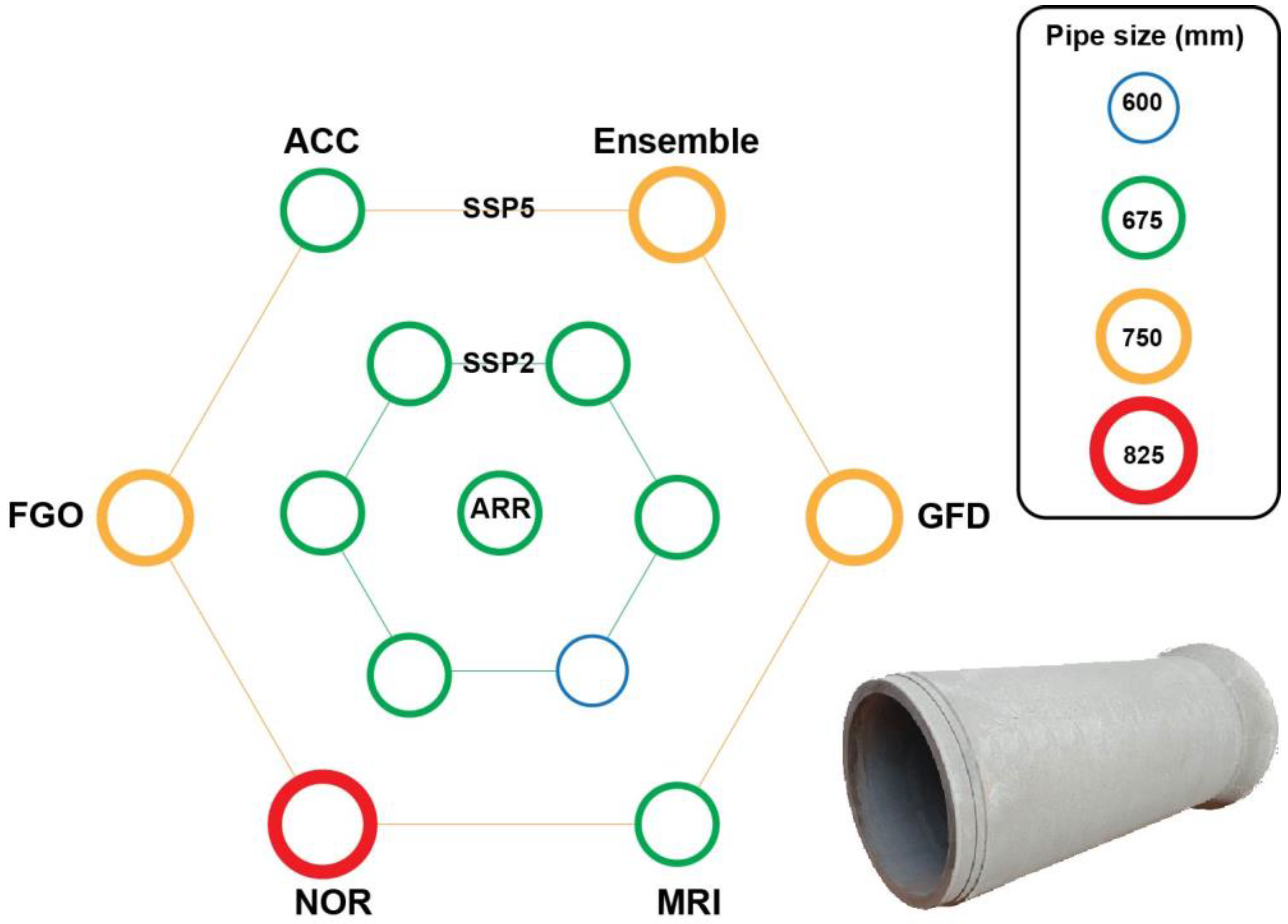
Figure 1. Methodology Framework.
Hydrology 10 00117 g001
Figure 2. Study Area.
Hydrology 10 00117 g002
Figure 3. eCDF of AMS for both observed and GCMs in the historical period (The abbreviations correspond to different GCMs: (a) ACC, (b) FGO, (c) GFD, (d) INM, (e) ITM, (f) MRI, (g) NOR).
Hydrology 10 00117 g003
Figure 4. Projected (2031–2060) 24 h PFs for the different return periods of all GCMs for two scenarios (green and red lines) compared to historical PFs of ARR (black line) for Sydney airport station ((a) corresponds to SSP2 and (b) corresponds to SSP5). For the historical PFs of ARR, the 2 yr IDF does not correspond to the 2-year average recurrence interval (ARI) IDF, and rather, it corresponds to the 1.44 ARI. Similarly, the 5 yr IDF corresponds to the 4.48 ARI [48].
Hydrology 10 00117 g004
Figure 5. Variations in projected 24 h PFs from the historical values of ARR for different GCMs in two scenarios at Sydney airport station ((a) corresponds to SSP2 and (b) corresponds to SSP5).
Hydrology 10 00117 g005
Figure 6. The size of culvert based on different GCMs and scenarios for the projected period, 2031–2060.
Hydrology 10 00117 g006
Table 1. Characteristics of the seven CMIP6 GCMs used in this study.
ModelModel AbbreviationContact InstitutionInstitution IDSpatial Resolution (lon × lat)
ACCESS-CM2ACCAustralian Community Climate and Earth-System SimulatorCSIRO1.875° × 1.25°
FGOALS-g3FGOChinese Academy of SciencesCAS2° × 2.25°
GFDL-ESM4GFDNOAA Geophysical Fluid Dynamics Laboratory, Princeton, New Jersey, USANOAA-GFDL1° × 1°
IITM-ESMITMIndian Institute of Tropical MeteorologyIITM1° × 1°
INM-CM5-0INMInstitute of Numerical Mathematics, Moscow, RussiaINM2° × 1.5°
MRI-ESM2-0MRIMeteorological Research Institute, Tsukuba, JapanMRI1.125° × 1.1215°
NorESM2-MMNORNorwegian Climate Service CentreNCC1.25° × 0.9424°
Table 2. Culvert design comparison for 1 h 100 yr rainfall event using historical, ARR, and projected PFs of the GCMs’ ensemble.
ARRSSP2SSP5
Rainfall intensity(mm/h)687495.7
Storm runoff (m3/s)0.490.530.69
Disclaimer/Publisher’s Note: The statements, opinions and data contained in all publications are solely those of the individual author(s) and contributor(s) and not of MDPI and/or the editor(s). MDPI and/or the editor(s) disclaim responsibility for any injury to people or property resulting from any ideas, methods, instructions or products referred to in the content.

