

Discerning Watershed Response to Hydroclimatic Extremes with a Deep Convolutional Residual Regressive Neural Network
 , , , and
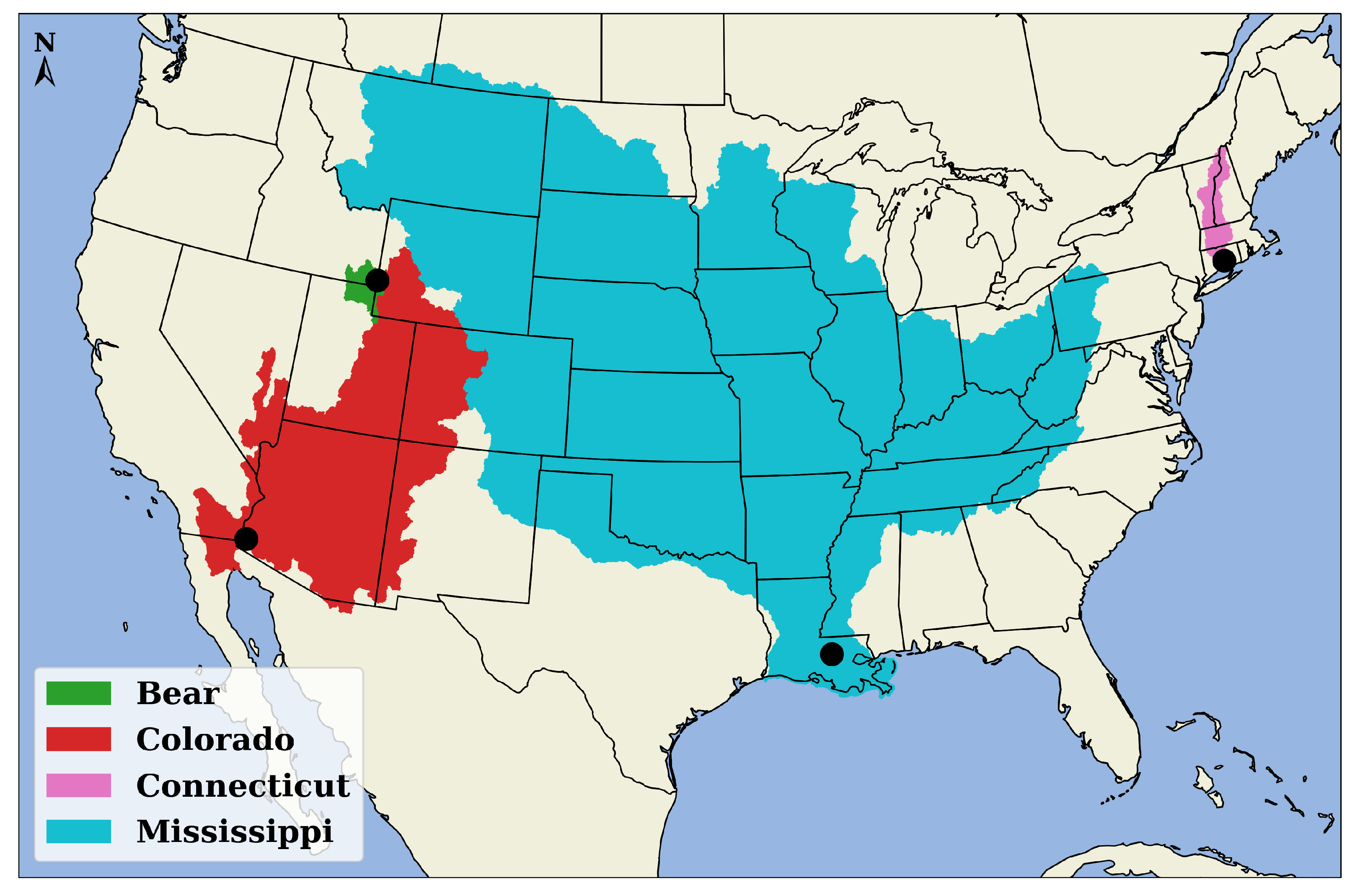
Abstract
:1. Introduction
2. Materials and Methods
2.1. Study Areas
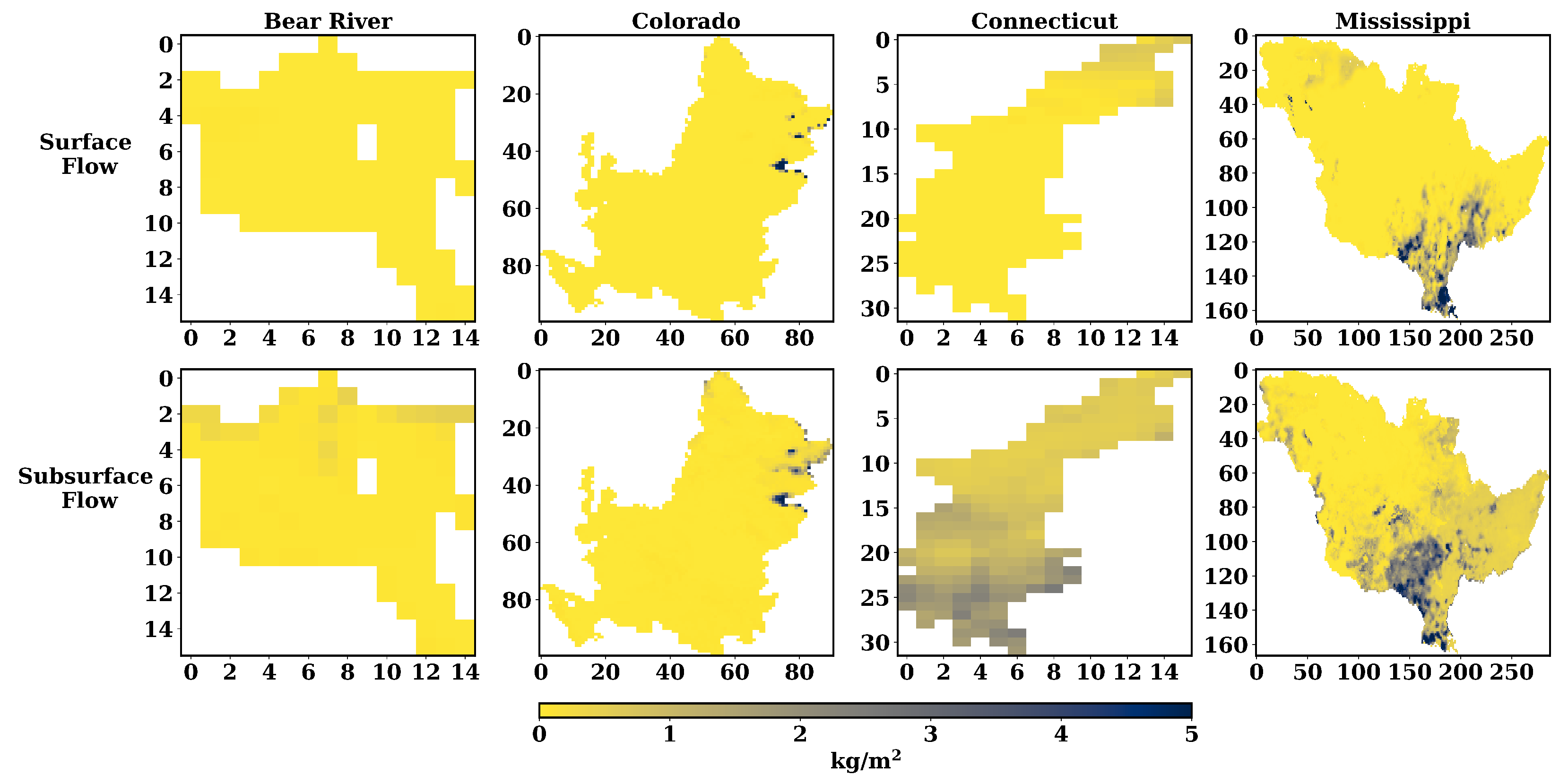
2.2. Satellite-Derived Observations
2.3. Ground-Truth Measurements
2.4. Data Collection and Preprocessing
2.5. Treatment
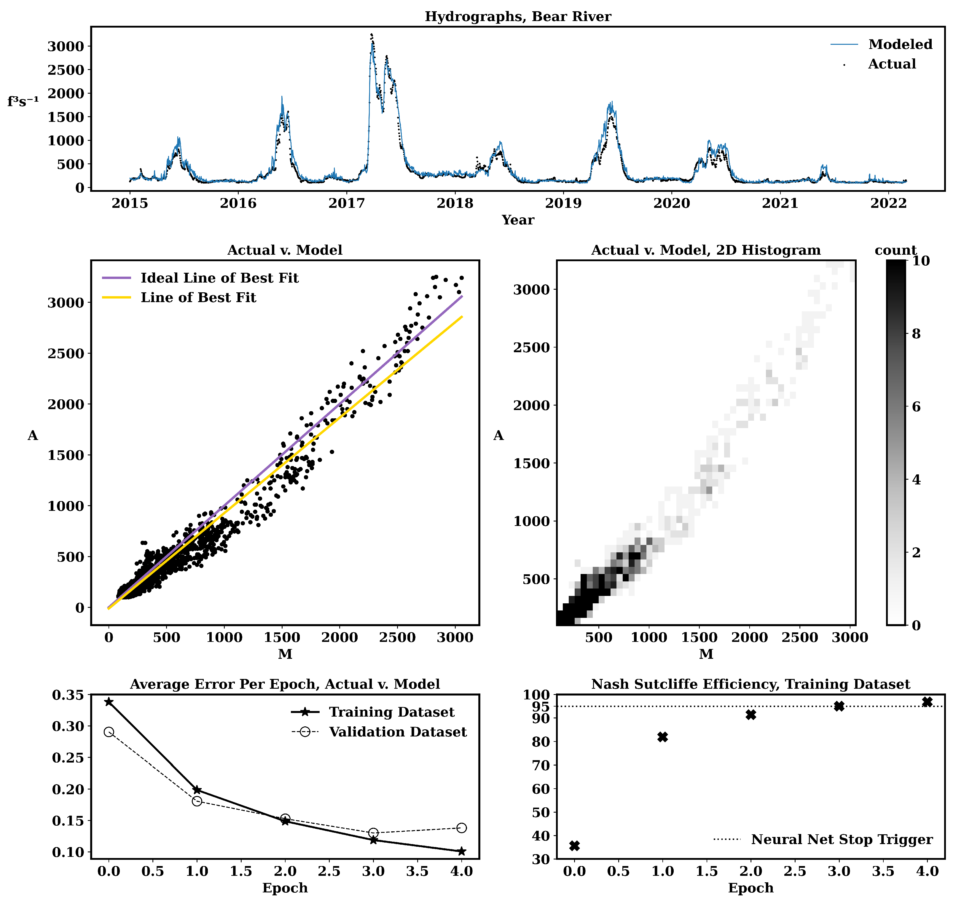
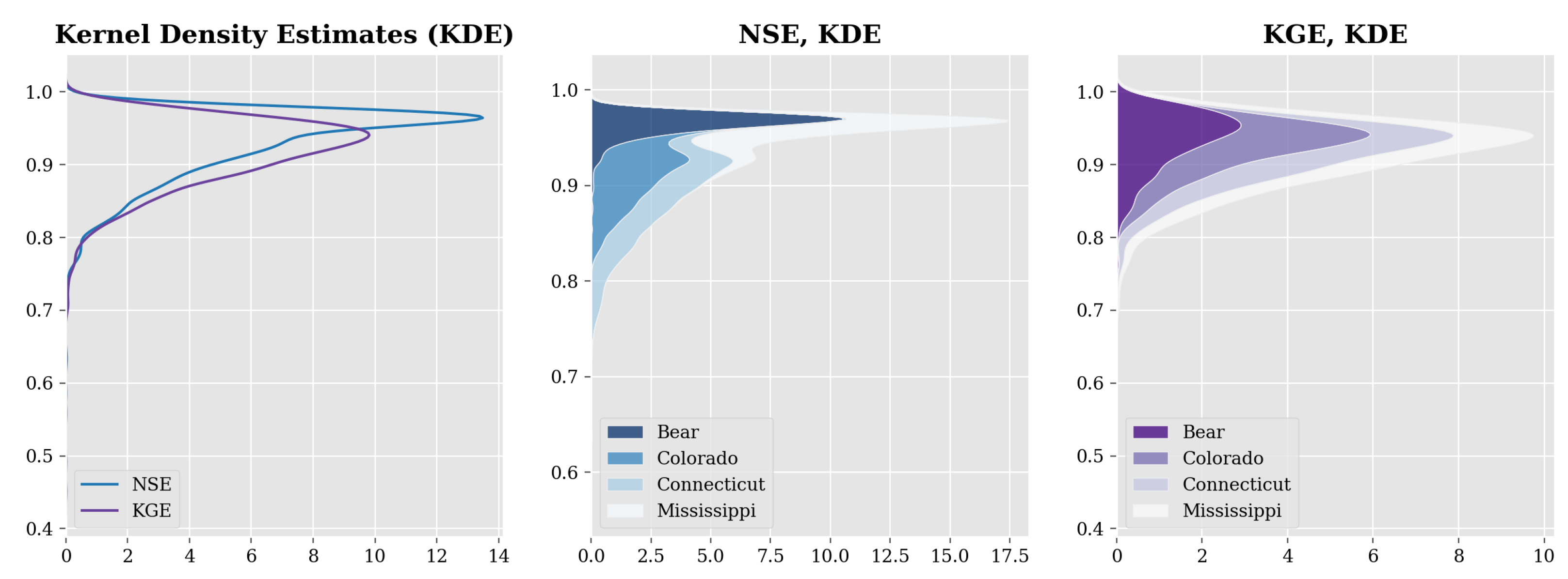
3. Results
4. Discussion
5. Conclusions
Author Contributions
Funding
Institutional Review Board Statement
Data Availability Statement
Acknowledgments
Conflicts of Interest
Abbreviations
| dcrrnn | deep convolutional residual regressive neural network |
| F2F | Flux to Flow |
| NASA | National Aeronautics and Space Administration |
| GLDAS | Global Land Data Assimilation System |
| NLDAS | National Land Data Assimilation System |
| USGS | United States Geological Survey |
| kg/m | kilograms per square meter |
| ft/s | cubic feet per second |
| A | actual gauged in the river measurement |
| M | modeled measurement via neural network |
| NSE | Nash–Sutcliffe efficiency |
| KGE | Kling–Gupta efficiency |
| KDE | kernel density estimate |
| TTS | training–test split |
References
- Stott, P. How climate change affects extreme weather events. Science 2016, 352, 1517–1518. [Google Scholar] [CrossRef] [PubMed]
- Qin, Y.; Abatzoglou, J.T.; Siebert, S.; Huning, L.S.; AghaKouchak, A.; Mankin, J.S.; Hong, C.; Tong, D.; Davis, S.J.; Mueller, N.D. Agricultural risks from changing snowmelt. Nat. Clim. Chang. 2020, 10, 459–465. [Google Scholar] [CrossRef]
- Min, C.; Yang, Q.; Chen, D.; Yang, Y.; Zhou, X.; Shu, Q.; Liu, J. The emerging Arctic shipping corridors. Geophys. Res. Lett. 2022, 45, e2022GL099157. [Google Scholar] [CrossRef]
- Tebaldi, C.; Ranasinghe, R.; Vousdoukas, M.; Rasmussen, D.; Vega-Westhoff, B.; Kirezci, E.; Kopp, R.E.; Sriver, R.; Mentaschi, L. Extreme sea levels at different global warming levels. Nat. Clim. Chang. 2021, 11, 746–751. [Google Scholar] [CrossRef]
- Sévellec, F.; Fedorov, A.V.; Liu, W. Arctic sea-ice decline weakens the Atlantic meridional overturning circulation. Nat. Clim. Chang. 2017, 7, 604–610. [Google Scholar] [CrossRef]
- Karl, T.R.; Nicholls, N.; Gregory, J. The coming climate. Sci. Am. 1997, 276, 78–83. [Google Scholar] [CrossRef]
- Underwood, E. Models predict longer, deeper US droughts. Science 2015, 347, 707. [Google Scholar] [CrossRef]
- Milly, P.C.D.; Wetherald, R.T.; Dunne, K.; Delworth, T.L. Increasing risk of great floods in a changing climate. Nature 2002, 415, 514–517. [Google Scholar] [CrossRef]
- Hirabayashi, Y.; Mahendran, R.; Koirala, S.; Konoshima, L.; Yamazaki, D.; Watanabe, S.; Kim, H.; Kanae, S. Global flood risk under climate change. Nat. Clim. Chang. 2013, 3, 816–821. [Google Scholar] [CrossRef]
- Parmesan, C.; Root, T.L.; Willig, M.R. Impacts of extreme weather and climate on terrestrial biota. Bull. Am. Meteorol. Soc. 2000, 81, 443–450. [Google Scholar] [CrossRef]
- Gleick, P.H.; Cooley, H. Freshwater Scarcity. Annu. Rev. Environ. Resour. 2021, 46, 319–348. [Google Scholar] [CrossRef]
- Crisp, N.H.; Roberts, P.C.; Livadiotti, S.; Oiko, V.T.A.; Edmondson, S.; Haigh, S.; Huyton, C.; Sinpetru, L.; Smith, K.; Worrall, S.; et al. The benefits of very low earth orbit for earth observation missions. Prog. Aerosp. Sci. 2020, 117, 100619. [Google Scholar] [CrossRef]
- Minzu, V.; Riahi, S.; Rusu, E. Optimal control of an ultraviolet water disinfection system. Appl. Sci. 2021, 11, 2638. [Google Scholar] [CrossRef]
- Horton, P.; Schaefli, B.; Kauzlaric, M. Why do we have so many different hydrological models? A review based on the case of Switzerland. Wiley Interdiscip. Rev. Water 2022, 9, e1574. [Google Scholar] [CrossRef]
- Abbaspour, K.C.; Yang, J.; Maximov, I.; Siber, R.; Bogner, K.; Mieleitner, J.; Zobrist, J.; Srinivasan, R. Modelling hydrology and water quality in the pre-alpine/alpine Thur watershed using SWAT. J. Hydrol. 2007, 333, 413–430. [Google Scholar] [CrossRef]
- Wang, Y.; Jiang, R.; Xie, J.; Zhao, Y.; Yan, D.; Yang, S. Soil and water assessment tool (SWAT) model: A systemic review. J. Coast. Res. 2019, 93, 22–30. [Google Scholar] [CrossRef]
- Beven, K.J.; Buytaert, W.; Smith, L.A.; Westerberg, I.K.; McMillan, H.K. A decade of Predictions in Ungauged Basins (PUB)—A review. Hydrol. Sci. J. 2013, 58, 1198–1255. [Google Scholar]
- Kiehl, J.T. Twentieth century climate model response and climate sensitivity. Geophys. Res. Lett. 2007, 34, L22710. [Google Scholar] [CrossRef]
- Vano, J.A.; Das, T.; Tague, C.; Padowski, J.; Udall, B.; Bart, R.; Klos, P.Z. Hydrologic implications of dynamical and statistical approaches to downscaling climate model outputs. Clim. Chang. 2013, 119, 519–539. [Google Scholar]
- Haidvogel, D.B.; Arango, H.G.; Hedstrom, K.S.; Beckmann, A.; Malanotte-Rizzoli, P.; Shchepetkin, A.F. Model evaluation experiments in the North Atlantic Basin: Simulations in nonlinear terrain-following coordinates. Dyn. Atmos. Ocean. 2008, 44, 28–48. [Google Scholar] [CrossRef]
- Marshall, J.; Adcroft, A.; Hill, C.; Perelman, L.; Heisey, C. A finite-volume, incompressible Navier Stokes model for studies of the ocean on parallel computers. J. Geophys. Res. Ocean. 1997, 102, 5753–5766. [Google Scholar] [CrossRef]
- Xia, Y.; Mitchell, K.; Ek, M.; Sheffield, J.; Cosgrove, B.; Wood, E.; Luo, L.; Alonge, C.; Wei, H.; Meng, J.; et al. Continental-scale water and energy flux analysis and validation for the North American Land Data Assimilation System project phase 2 (NLDAS-2): 1. Intercomparison and application of model products. J. Geophys. Res. Atmos. 2012, 117, D03109. [Google Scholar] [CrossRef]
- Liang, X.; Lettenmaier, D.P.; Wood, E.F.; Burges, S.J. A simple hydrologically based model of land surface water and energy fluxes for general circulation models. J. Geophys. Res. Atmos. 1994, 99, 14415–14428. [Google Scholar] [CrossRef]
- Ries, K.G. The national water information system: A United States government water data infrastructure. Int. J. River Basin Manag. 2015, 13, 289–298. [Google Scholar]
- Mueller, D.K.; Wagner, R.J.; Nystrom, E.A. Overview of the United States Geological Survey National Water Information System database. J. Water Resour. Plan. Manag. 2016, 142, 05016004. [Google Scholar]
- Stewart, D.W.; Caldwell, R.R.; Hunt, R.J.; Viger, R.J. The US Geological Survey’s Water Availability and Use Science Program: Overview and selected research activities. US Geol. Surv. Fact Sheet 2018, 2018, 1–6. [Google Scholar]
- Benson, M.A.; Carter, J.M.; Ritzman, R.A.; Landers, M.N. US Geological Survey stream-gaging program: Overview and highlights, 1879–2007. US Geol. Surv. Circ. 2009, 1331, 1–60. [Google Scholar]
- Hirsch, R.M.; De Cicco, L.A. USGS streamgages and US Environmental Protection Agency water quality monitoring: A successful partnership. Environ. Monit. Assess. 2010, 171, 21–27. [Google Scholar]
- Karhunen, J.; Oja, E.; Wang, L.; Vigario, R.; Joutsensalo, J. A class of neural networks for independent component analysis. IEEE Trans. Neural Netw. 1997, 8, 486–504. [Google Scholar] [CrossRef]
- Chen, Z.; Bei, Y.; Rudin, C. Concept whitening for interpretable image recognition. Nat. Mach. Intell. 2020, 2, 772–782. [Google Scholar] [CrossRef]
- He, K.; Zhang, X.; Ren, S.; Sun, J. Deep residual learning for image recognition. In Proceedings of the IEEE Conference on Computer Vision and Pattern Recognition, Las Vegas, NV, USA, 27–30 June 2016; pp. 770–778. [Google Scholar]
- Weiss, K.; Khoshgoftaar, T.M.; Wang, D. A survey of transfer learning. J. Big Data 2016, 3, 9. [Google Scholar] [CrossRef]
- David, C.H.; Maidment, D.R.; Niu, G.Y.; Yang, Z.L.; Habets, F.; Eijkhout, V. River network routing on the NHDPlus dataset. J. Hydrometeorol. 2011, 12, 913–934. [Google Scholar] [CrossRef]
- PyTorch. PyTorch: Deep Learning with PyTorch. Available online: https://pytorch.org/tutorials/beginner/deep_learning_60min_blitz.html (accessed on 30 March 2023).
- Rawat, W.; Wang, Z. Deep convolutional neural networks for image classification: A comprehensive review. Neural Comput. 2017, 29, 2352–2449. [Google Scholar] [CrossRef] [PubMed]
- Agarap, A.F. Deep learning using rectified linear units (relu). arXiv 2018, arXiv:1803.08375. [Google Scholar]
- Ioffe, S.; Szegedy, C. Batch normalization: Accelerating deep network training by reducing internal covariate shift. In International Conference on Machine Learning; PMLR: London, UK, 2015; pp. 448–456. [Google Scholar]
- Amari, S.i. Backpropagation and stochastic gradient descent method. Neurocomputing 1993, 5, 185–196. [Google Scholar] [CrossRef]
- Kingma, D.P.; Ba, J. Adam: A method for stochastic optimization. arXiv 2014, arXiv:1412.6980. [Google Scholar]
- Nash, J.E.; Sutcliffe, J.V. River flow forecasting through conceptual models part I—A discussion of principles. J. Hydrol. 1970, 10, 282–290. [Google Scholar] [CrossRef]
- Gupta, H.; Kling, H.; Yilmaz, K.; Martinez, G. Decomposition of the mean squared error and NSE performance criteria: Implications for improving hydrological modelling. J. Hydrol. 2009, 377, 80–91. [Google Scholar] [CrossRef]
- Gupta, H.; Kling, H. On typical range, sensitivity, and normalization of Mean Squared Error and Nash-Sutcliffe Efficiency type metrics. Water Resour. Res. 2011, 47, W10601. [Google Scholar] [CrossRef]
- Knoben, W.J.; Freer, J.E.; Woods, R.A. Inherent benchmark or not? Comparing Nash–Sutcliffe and Kling–Gupta efficiency scores. Hydrol. Earth Syst. Sci. 2019, 23, 4323–4331. [Google Scholar] [CrossRef]
- Van Der Ent, R.J.; Tuinenburg, O.A. The residence time of water in the atmosphere revisited. Hydrol. Earth Syst. Sci. 2017, 21, 779–790. [Google Scholar] [CrossRef]
- Gimeno, L.; Eiras-Barca, J.; Durán-Quesada, A.M.; Dominguez, F.; van der Ent, R.; Sodemann, H.; Sánchez-Murillo, R.; Nieto, R.; Kirchner, J.W. The residence time of water vapour in the atmosphere. Nat. Rev. Earth Environ. 2021, 2, 558–569. [Google Scholar] [CrossRef]
- Qi, J.; Wang, Q.; Zhang, X. On the use of NLDAS2 weather data for hydrologic modeling in the Upper Mississippi River Basin. Water 2019, 11, 960. [Google Scholar] [CrossRef]
- Chen, M.; Cui, Y.; Gassman, P.W.; Srinivasan, R. Effect of watershed delineation and climate datasets density on runoff predictions for the Upper Mississippi River Basin using SWAT within HAWQS. Water 2021, 13, 422. [Google Scholar] [CrossRef]
- Tran, H.; Zhang, J.; O’Neill, M.M.; Ryken, A.; Condon, L.E.; Maxwell, R.M. A hydrological simulation dataset of the Upper Colorado River Basin from 1983 to 2019. Sci. Data 2022, 9, 16. [Google Scholar] [CrossRef]
- Cai, X.; Yang, Z.L.; Xia, Y.; Huang, M.; Wei, H.; Leung, L.R.; Ek, M.B. Assessment of simulated water balance from Noah, Noah-MP, CLM, and VIC over CONUS using the NLDAS test bed. J. Geophys. Res. Atmos. 2014, 119, 13–751. [Google Scholar] [CrossRef]
- Yang, F.; Cerrai, D.; Anagnostou, E.N. The effect of lead-time weather forecast uncertainty on outage prediction modeling. Forecasting 2021, 3, 501–516. [Google Scholar] [CrossRef]
- Jiang, X.; Adames, Á.F.; Kim, D.; Maloney, E.D.; Lin, H.; Kim, H.; Zhang, C.; DeMott, C.A.; Klingaman, N.P. Fifty years of research on the Madden-Julian Oscillation: Recent progress, challenges, and perspectives. J. Geophys. Res. Atmos. 2020, 125, e2019JD030911. [Google Scholar] [CrossRef]
- Hu, D.; Wu, L.; Cai, W.; Gupta, A.S.; Ganachaud, A.; Qiu, B.; Gordon, A.L.; Lin, X.; Chen, Z.; Hu, S.; et al. Pacific western boundary currents and their roles in climate. Nature 2015, 522, 299–308. [Google Scholar] [CrossRef]
- Ionita, M.; Nagavciuc, V.; Scholz, P.; Dima, M. Long-term drought intensification over Europe driven by the weakening trend of the Atlantic Meridional Overturning Circulation. J. Hydrol. Reg. Stud. 2022, 42, 101176. [Google Scholar] [CrossRef]
- Siders, A.R. Social justice implications of US managed retreat buyout programs. Clim. Chang. 2019, 152, 239–257. [Google Scholar] [CrossRef]
- Hino, M.; Field, C.B.; Mach, K.J. Managed retreat as a response to natural hazard risk. Nat. Clim. Chang. 2017, 7, 364–370. [Google Scholar] [CrossRef]
- GulfNews. Death Toll from Pakistan Floods Reaches 25. Gulf News, 5 September 2022.
- CBS. Flooding across Mississippi Amid Heavy Rainfall. CBS News, 29 August 2022.
- Blake, E.S.; Gibney, E.J.; Center, N.H. Hurricane Harvey: 17–31 August 2017. Mon. Weather. Rev. 2018, 146, 3605–3609. [Google Scholar]
- Elsner, J.B.; Basu, S.; Fragomeni, M.V. Projected Atlantic hurricane surge threat from rising temperatures. Environ. Res. Lett. 2020, 15, 014014. [Google Scholar]
- Charrua, A.B.; Padmanaban, R.; Cabral, P.; Bandeira, S.; Romeiras, M.M. Impacts of the tropical cyclone idai in mozambique: A multi-temporal landsat satellite imagery analysis. Remote Sens. 2021, 13, 201. [Google Scholar] [CrossRef]
- Parks, R.; McLaren, M.; Toumi, R.; Rivett, U. Experiences and Lessons in Managing Water from Cape Town; Grantham Institute Briefing Paper No. 29; Imperial College London: London, UK, 2019; pp. 1–20. [Google Scholar]
- Zhao, C.; Wang, G.; Zhang, M.; Wang, G.; de With, G.; Bezhenar, R.; Maderich, V.; Xia, C.; Zhao, B.; Jung, K.T.; et al. Transport and dispersion of tritium from the radioactive water of the Fukushima Daiichi nuclear plant. Mar. Pollut. Bull. 2021, 169, 112515. [Google Scholar] [CrossRef]
- Machida, M.; Yamaguchi, T.; Okuda, K. Current and historical cesium distribution in sediments in Fukushima coastal estuaries: Impact of a mega-typhoon on the remobilization and accumulation of radiocesium. J. Environ. Radioact. 2018, 189, 109–116. [Google Scholar] [CrossRef]
- Ghosh, S.; Islam, M.R.; Danish, M.S.S. A review of early warning systems for urban flood management. J. Hydrol. 2017, 548, 672–691. [Google Scholar] [CrossRef]
- Goodwill, J.E.; Ray, P.; Nock, D.; Miller, C.M. Emerging investigator series: Moving beyond resilience by considering antifragility in potable water systems. Environ. Sci. Water Res. Technol. 2022, 8, 8–21. [Google Scholar] [CrossRef]
- Vogel, J.; Åkesson, A.; Bohnenstengel, K. Evaluating the impact of blue-green infrastructure on urban flooding in southeast Norway using hydrodynamic modelling. Sustainability 2019, 11, 335. [Google Scholar] [CrossRef]
- CBD. Convention on Biological Diversity-Nature-Based Solutions. 2019. Available online: https://www.cbd.int (accessed on 11 April 2023).
- Ebi, K.L.; Ford, J.D. Inequalities in heat-related mortality in a warming world: The role of adaptive capacity. Curr. Epidemiol. Rep. 2019, 6, 61–69. [Google Scholar]
- Masson-Delmotte, V.; Zhai, P.; Pörtner, H.O.; Roberts, D.; Skea, J.; Shukla, P.R.; Pirani, A.; Moufouma-Okia, W.; Péan, C.; Pidcock, R.; et al. Global warming of 1.5 C. IPCC Spec. Rep. Impacts Glob. Warm. 2018, 1, 43–50. [Google Scholar]
- Xia, Y.; Ek, M.; Wei, H.; Meng, J. Comparative analysis of relationships between NLDAS-2 forcings and model outputs. Hydrol. Process 2012, 26, 467–474. [Google Scholar] [CrossRef]
- East, A.E.; Stevens, A.W.; Ritchie, A.C.; Barnard, P.L.; Campbell-Swarzenski, P.; Collins, B.D.; Conaway, C.H. A regime shift in sediment export from a coastal watershed during a record wet winter, California: Implications for landscape response to hydroclimatic extremes. Earth Surf. Process. Landf. 2018, 43, 2562–2577. [Google Scholar] [CrossRef]
- Brown, C.F.; Brumby, S.P.; Guzder-Williams, B.; Birch, T.; Hyde, S.B.; Mazzariello, J.; Czerwinski, W.; Pasquarella, V.J.; Haertel, R.; Ilyushchenko, S.; et al. Dynamic World, Near real-time global 10 m land use land cover mapping. Sci. Data 2022, 9, 251. [Google Scholar] [CrossRef]
- Derakhshani, R.; Zaresefat, M.; Nikpeyman, V.; GhasemiNejad, A.; Shafieibafti, S.; Rashidi, A.; Nemati, M.; Raoof, A. Machine Learning-Based Assessment of Watershed Morphometry in Makran. Land 2023, 12, 776. [Google Scholar] [CrossRef]
- Hosseinzadeh, P.; Nassar, A.; Boubrahimi, S.F.; Hamdi, S.M. ML-Based Streamflow Prediction in the Upper Colorado River Basin Using Climate Variables Time Series Data. Hydrology 2023, 10, 29. [Google Scholar] [CrossRef]
- Khan, S.; Naseer, M.; Hayat, M.; Zamir, S.W.; Khan, F.S.; Shah, M. Transformers in vision: A survey. ACM Comput. Surv. (CSUR) 2022, 54, 1–41. [Google Scholar] [CrossRef]


Disclaimer/Publisher’s Note: The statements, opinions and data contained in all publications are solely those of the individual author(s) and contributor(s) and not of MDPI and/or the editor(s). MDPI and/or the editor(s) disclaim responsibility for any injury to people or property resulting from any ideas, methods, instructions or products referred to in the content. |
© 2023 by the authors. Licensee MDPI, Basel, Switzerland. This article is an open access article distributed under the terms and conditions of the Creative Commons Attribution (CC BY) license (https://creativecommons.org/licenses/by/4.0/).
Share and Cite
Larson, A.; Hendawi, A.; Boving, T.; Pradhanang, S.M.; Akanda, A.S. Discerning Watershed Response to Hydroclimatic Extremes with a Deep Convolutional Residual Regressive Neural Network. Hydrology 2023, 10, 116. https://doi.org/10.3390/hydrology10060116
Larson A, Hendawi A, Boving T, Pradhanang SM, Akanda AS. Discerning Watershed Response to Hydroclimatic Extremes with a Deep Convolutional Residual Regressive Neural Network. Hydrology. 2023; 10(6):116. https://doi.org/10.3390/hydrology10060116
Chicago/Turabian StyleLarson, Albert, Abdeltawab Hendawi, Thomas Boving, Soni M. Pradhanang, and Ali S. Akanda. 2023. "Discerning Watershed Response to Hydroclimatic Extremes with a Deep Convolutional Residual Regressive Neural Network" Hydrology 10, no. 6: 116. https://doi.org/10.3390/hydrology10060116