Article

Developing a Modified Online Water Quality Index: A Case Study for Brazilian Reservoirs

by
Pamela Lais Cabral Silva
,
Alisson Carraro Borges
*,
Lucas Sampaio Lopes
and
André Pereira Rosa
Department of Agricultural Engineering, Federal University of Viçosa, Viçosa 36570-000, MG, Brazil
*
Author to whom correspondence should be addressed.
Hydrology 2023, 10(6), 115; https://doi.org/10.3390/hydrology10060115
Submission received: 12 April 2023 / Revised: 15 May 2023 / Accepted: 17 May 2023 / Published: 23 May 2023
(This article belongs to the Special Issue Advances in River Monitoring)

Abstract

:
Online approaches for monitoring water quality can be an alternative aid to rapid decision-making in watershed management, especially reservoirs, given their vulnerability to the process of eutrophication. In this study, a modified water quality index (WQI) was developed using parameters that are easily measured with sensors, which would allow for the online monitoring of reservoirs. The modified WQI was based on WQICETESB and we used regression models to obtain values for the parameters: total phosphorus (TP), total nitrogen (TN), biochemical oxygen demand (BOD) and total solids (TS). Water quality data from reservoirs from 2003 to 2020 were used, which were provided by the Environmental Company of the State of São Paulo (CETESB), Brazil. The adjusted modified WQI employing weight redistribution (WQIRWAdj or WQISOL) presented the most promising results, with a Pearson correlation of 0.92 and a success rate of 72.6% and 97.0% for the CETESB and simplified classifications, respectively. WQISOL, which was proposed in the present study, exhibited a satisfactory performance, allowing the water quality of reservoirs to be monitored remotely and in real-time.

1. Introduction

Currently, there is a reduction in the availability of surface water due to degradation from anthropogenic activities and natural processes. According to Boretti and Rosa [1], water resources suitable for human consumption will be scarce by 2050. This scarcity will make it impossible to use water for multiple purposes, including human consumption, industrial and agricultural use, and even for recreational purposes [2,3,4]. As a result, water resource management has been increasing, and action to prevent the degradation of surface water bodies has taken a prominent role.
The use of tools to monitor surface water has proven advantageous from environmental, health, and economic standpoints, as they help safeguard the quality of this essential and irreplaceable resource [4,5]. Such monitoring is fundamental to water resource management, as it can indicate trends in the loss of water quality and point out possible sources of pollution [6].
One tool that is widely used around the world to evaluate and optimize the monitoring of surface water quality is the water quality index (WQI) [7,8,9,10,11]. Such indices consist of mathematical techniques that gather various parameters into a single value, enabling water quality to be classified in a simple way that is easy for the general population to understand [3,6]. In recent years, various new approaches have been reported regarding WQI, for example, using the concepts of entropy in WQI for groundwater and surface water assessments [8,9] and the incorporation of health risk assessments [10].
Despite the advantages, obtaining the necessary parameters for WQIs use may make the periodic monitoring of water quality a laborious and costly task [6,12,13]. Due to these obstacles, the development of tools that allow accurate, simultaneous results and that require a smaller range of parameters can result in more efficient monitoring of water quality [6].
In this respect, WQIs that are modified to only include water parameters that can be measured using analytical instruments are promising, as they allow the quality to be monitored remotely and in real-time and dispensed with methodologies that include analyses using toxic and dangerous reagents. In light of these aspects, this study aimed to obtain an online water quality index that would allow remote and real-time water quality monitoring in reservoirs.

2. Materials and Methods

2.1. Sampling

The state of São Paulo, located in southeastern Brazil, has a strong tradition of monitoring its water bodies, resulting in a larger volume of water quality data compared to other Brazilian states. São Paulo is home to an expressive resident population of 46.29 million people and has the highest number of industrial establishments in Brazil, making it an important area for the study of water pollution sources. This study focused on 32 reservoirs with 48 monitoring points (Figure 1), and the water quality data were obtained from CETESB’s basic network of surface water monitoring in the InfoÁguas platform. The dataset included information on several water quality parameters. In addition, the database contained information on sampling points, altitude, and sampling dates, providing a comprehensive picture of water quality in the state of São Paulo. The data provided a valuable source of information for the development of a modified representative WQI, which could help assess and manage the quality of water resources in the state and ensure their sustainable use and conservation.
The study used seven explanatory variables, including electrical conductivity (EC), nitrate nitrogen (NO3-N), ammoniacal nitrogen (NH3-N), dissolved oxygen (DO), hydrogenionic potential (pH), water temperature (T), and turbidity (Turb). These parameters can be measured directly by analytical instruments. Sampling dates for determining the precipitation regime were also included. The response variables of the regression models are biochemical oxygen demand (BOD), total phosphorus (TP), total nitrogen (TN), coliforms, and total solids (TS). These water quality parameters have complex measurement methodologies.
It is important to note that adjustments were made to the TN and thermotolerant coliforms (TC) data due to changes in the methodology used by CETESB over the 18-year period. As such, TN was determined using the sum of total Kjeldahl nitrogen (TKN) and NO3-N, and the TC counts was transformed into E. coli using a correction factor of 1.25 proposed by CETESB itself [14,15,16]. Regarding outliers in time series, when necessary, the robust regression followed by the outlier identification (ROUT) method was used.

2.2. Regression Models for BOD, TP, TN, Coliforms, and TS Predictions

A time series from 2008 to 2017 was used to construct the predictive models. The correlations between the pre-selected explanatory variables (EC, NO3-N, NH3-N, DO, pH, T, and Turb) and the target variables (TP, TN, coliforms, and TS) were carried out using the Spearman’s correlation analysis [17]. As the precipitation regime is a dichotomous variable (D), the dummy method [18] was used to include the influence of precipitation in the regression models. Here, D assumes a value equal to one for rainy periods and a value equal to zero for dry periods. The period from April to September is characterized as the dry season, and from October to March as the rainy season.
The prediction efficiency of the constructed models was evaluated using the coefficient of determination (R2) and the adjusted coefficient of determination (R2adj). The models were further cross-validated using the time series from 2018 to 2020, considering the above metrics and the Nash–Sutcliffe coefficient (NSE), and the Pearson correlation coefficient [19,20,21]. This step was aimed at replacing complex monitoring variables with simpler ones in the process of obtaining the WQI.

2.3. Online Modified Water Quality Index

The modified WQI was based on the WQI adopted by CETESB. Therefore, Equation (1) and the quality charts constructed by CETESB were used to obtain the quality of parameter i (qi). Detailed explanations about the process of calculating the scores for each water quality category and regarding the color ranges are available on the CETESB website: www.cetesb.sp.gov.br/aguas-interiores/wp-content/uploads/sites/12/2013/11/02.pdf [22].
W Q I = i = 1 n q i w i
where
WQI = water quality index, is a score that indicates water quality, expressed as a number between 0 and 100;
qi = quality of the ith parameter, a number between 0 and 100, obtained from the respective ‘mean-value curve of the variation in quality’ as a function of its concentration;
wi = weight is corresponding to the ith parameter, a number between 0 and 1, assigned based on importance to the overall conformation with water quality.
The predictive models that exhibited the best performance were used to construct the modified WQIs for carrying out remote and online monitoring. The efficiency of these WQIs was evaluated by comparing the resulting classifications with those of WQICETESB (Table 1), the modified WQIs, and the WQIs proposed by Naveedullah et al. [4], Pesce and Wunderlin [23], and Moscuzza et al. [24].
A linear regression adjustment was performed to enhance the performance of the modified WQIs. Furthermore, the modified WQIs were cross-validated using the time series from 2003 to 2007 to confirm whether the good performance observed during validating of the regression models would be replicated with other datasets.

3. Results and Discussion

3.1. Developing Regression Models to Be Used in Modified WQIs

Spearman’s correlation analysis was used to verify the possible relationships between the parameters of the water under study. Table 2 shows the results obtained from this analysis. Only correlations greater or equal to 0.4 (in bold) in absolute terms were considered. It was observed that eligible parameters could be used to compose predictive models for BOD, TN, TP, and TS concentrations. Very weak correlations were obtained for coliform values, and this variable was then disregarded.
Moderate positive ρ correlations between BOD and EC (0.4141), BOD and NH3-N (0.4982), and BOD and turbidity (0.4643) were observed. Additionally, TP exhibited positive moderate correlations with EC (0.5181), NH3-N (0.4626), and turbidity (0.5265). TN exhibited significant correlations with NH3-N (0.5343), NO3-N (0.4553), and turbidity (0.4201). Notably, EC exhibited a strong positive correlation (coefficient of 0.7041) with TN. These observed correlations for BOD, TP, and TN may be attributed to the discharge of domestic wastewater and agricultural runoff, which are major sources of organic matter and nutrients [25,26,27,28,29,30].
TS in water could be influenced by several direct or indirect factors. Although EC has a high correlation with TS (0.728), which can be explained by the known relationship between EC and total dissolved solids (TDS) [27,30], it may not reflect the trues relationship between them in some situations. Therefore, a simple linear regression based on only one variable (EC) may not capture the complexity and variability of water quality. To avoid these problems and to obtain a more accurate and robust predictive model of TS, we used multiple linear regression with all the available variables as predictors. This way, we were able to account for possible interactions and confounding effects among the variables and improve the explanatory power of the model.
The predictive models constructed using the time series from 2008 to 2017 are shown in Table 3.
Regression models are generally adjusted to predict responses for new observations, plot the relationships between variables, or find values that optimize one or more responses. The proposed models were, therefore, adjusted to describe the relationships found between the explanatory variables and the response variable through the regression of generalized linear models. Table 4 shows the results of the metrics obtained when adjusting the models.
Note that the regressions constructed for each of the parameters obtained an excellent fit between the predicted and observed values, as they presented coefficients of determination greater than 0.60. According to Barros Neto [28], this result indicates that the models can be used for predictive purposes, allowing the equations to estimate the concentrations of BOD, TP, TN, and TS.
Model validation aims to evaluate the performance of equations with datasets that are different to that used in developing the model. To determine the magnitude of the associated distortion, cross-validation was carried out using the coefficient of determination (R2) and the adjusted coefficient of determination (R2adj). To confirm the good performance of the model, the Pearson correlation (r) and the Nash–Sutcliffe coefficient of efficiency (NSE) were used with data collected between 2018 and 2020.
Table 5 shows the coefficients of the adjusted regression models, the coefficients of the validated models, and the NSE for each response variable. NSE values range from negative infinity to one, with higher values indicating better model performance, while lower or negative values suggest poorer model performance [21]. Values less than 0.36 are considered unsatisfactory, while values between 0.36 to 0.75 are classified as good, and values greater than 0.75 are regarded as excellent [29].
Each of the parameters exhibited an R2 and R2adj value greater than 0.60, indicating a good fit between the observed and predicted data. This means that the values estimated by the model were close to those observed during the period. Additionally, it should be noted that the coefficients of determination when validating were greater than those found when modeling. Hence, the models not only fit the new data but also maintained their performance using other sets of data than those used in their construction.
The Pearson correlation (r) for the parameters was close to 1, indicating that for each unit added in one group, there was a proportional increase in the other group. Additionally, the NSE confirmed a similar behavior to that found for the aforementioned metrics. All the parameters showed acceptable performance based on the range of values (0.36–0.75) shown in the literature [18]. It should be noted that the models for TP, TN, and TS obtained an NSE beyond this range and were considered to have good performance.
The regression models were proven to be suitable for predicting the values from laboratory procedures and they can make the process of monitoring water quality more practical and economically viable [
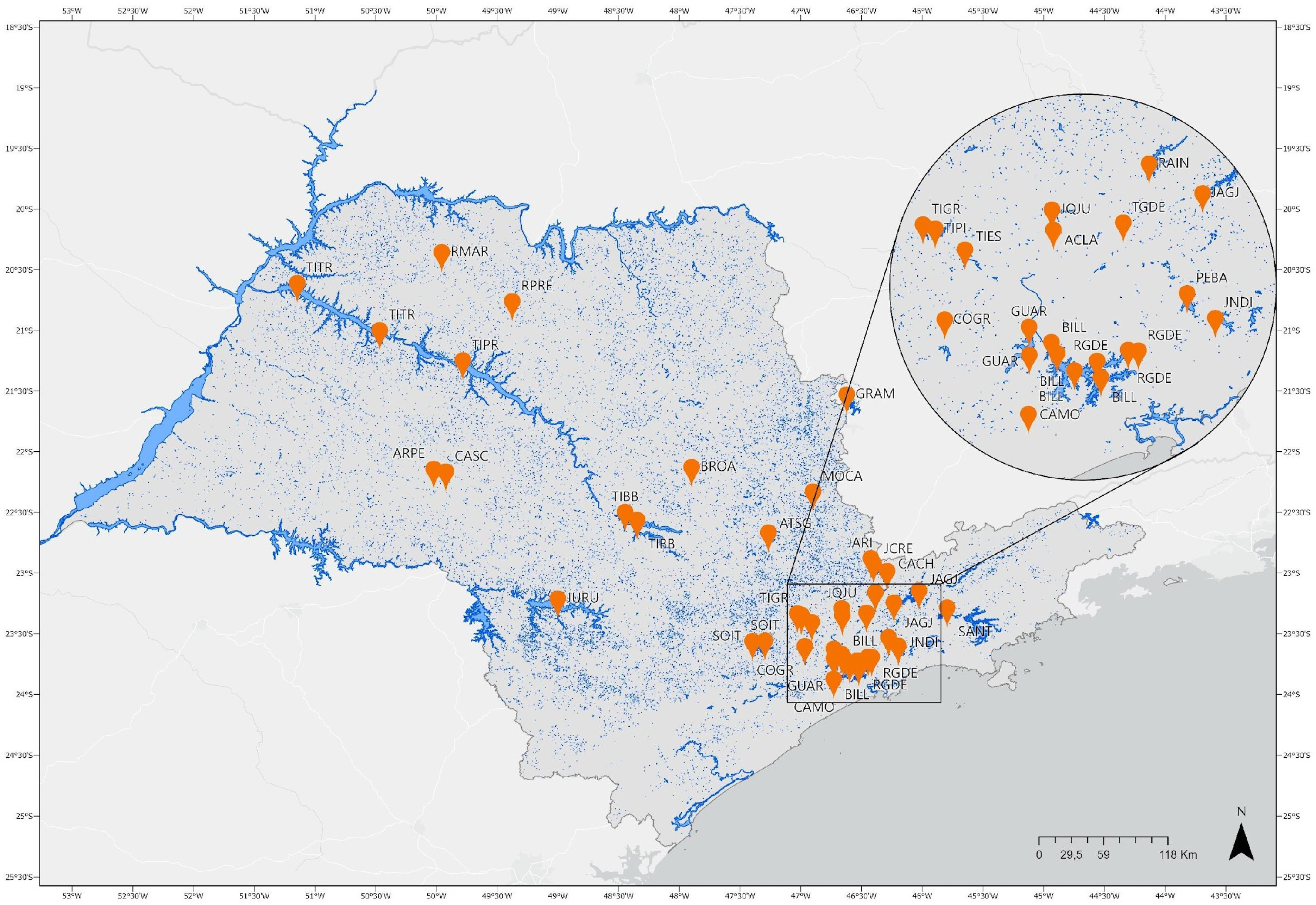
6]. Additionally, the results demonstrate that the regression models obtained in the present study should perform well with datasets of water quality from reservoirs under similar conditions to those found in the state of São Paulo, southeast of Brazil.

3.2. Online Modified Water Quality Indices

In constructing the online modified WQI indices, a decision was made to exclude the thermotolerant coliforms (TC) parameter, including its E. coli subset, due to the complexity of obtaining reliable predictive models [31,32,33,34]. To overcome the omission of TC when calculating the modified WQIs, two strategies were employed. The first strategy involved assigning new weights to each of the parameters that were retained, as presented in Table 6. The second strategy involved weighted redistribution of all the remaining variables, following the methodology proposed by Srivastava et al. [35].
DO was assigned the highest weight among the parameters that were retained, as it is a key indicator of water quality degradation and loss. Turbidity, which is often, but not exclusively, related to bacterial contamination, obtained a relatively high value compared to the original weights of WQICETESB. In addition, pH was also given a high weight due to its potential to indicate the discharge of industrial wastewater and significant disturbances in aquatic ecosystems [24,27].
Using the aforementioned methods, the modified WQIs values were calculated, and the resulting values were evaluated using a dataset of water quality data for reservoirs in the state of São Paulo between 2018 and 2020. Table 7 presents the correlation between WQICETESB values and the values obtained through the modified WQIs calculations, using both assigned weights (WQIAW) and the redistributed weights (WQIRW).
The results demonstrate a high and statistically significant correlation between the original WQICETESB values and the values obtained through the modified WQI calculations, using both the assigned and redistributed weights. This suggests that, despite the omission of TC and the use of estimated concentrations through the regression models, the modified WQIs produced values that closely approximated those obtained using the original CETESB methodology.
Subsequently, water quality classifications made by the reference WQI and the modified WQIs were analyzed to evaluate the efficacy of the proposed WQIs in terms of the range (color) classification presented in Table 1. 
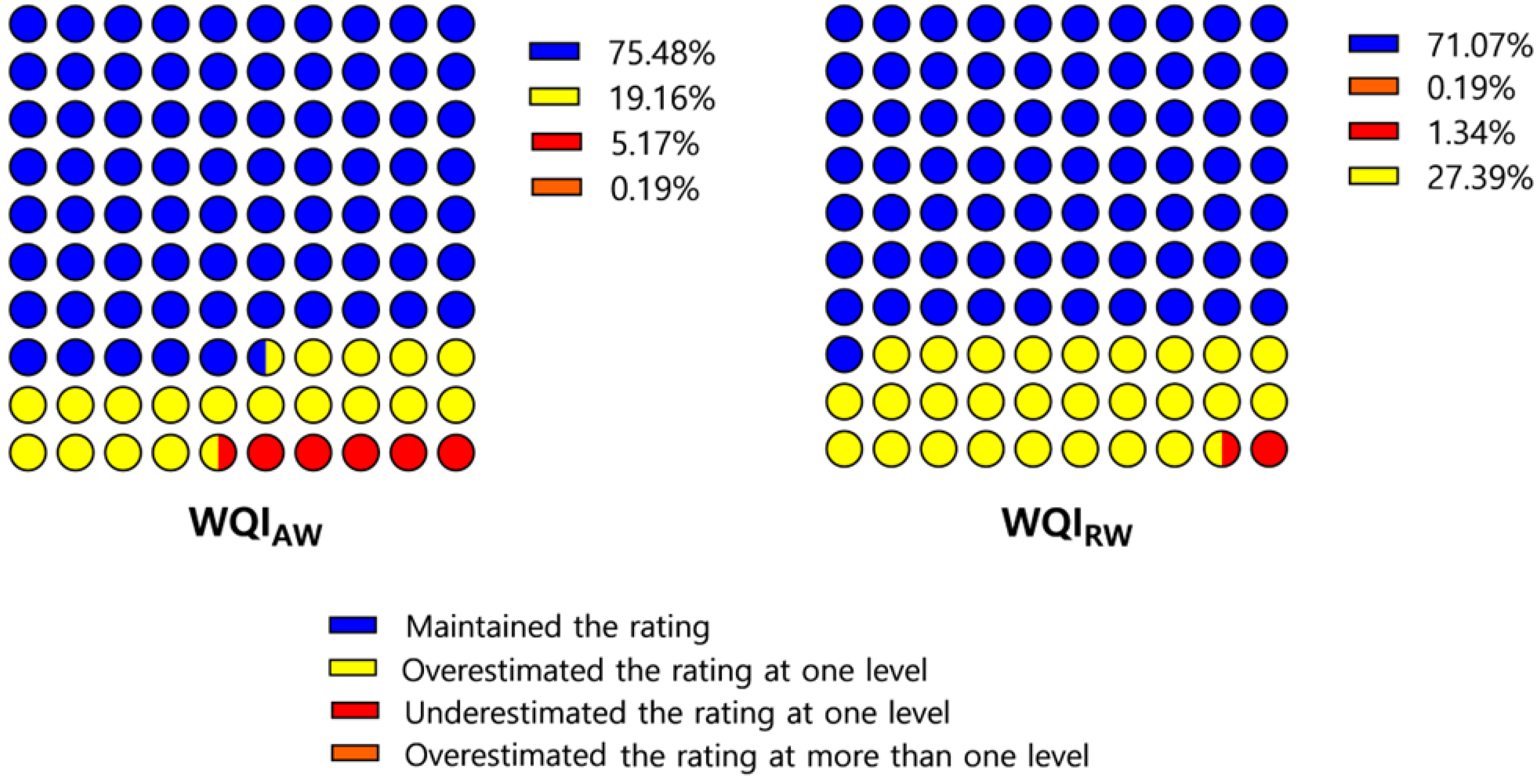
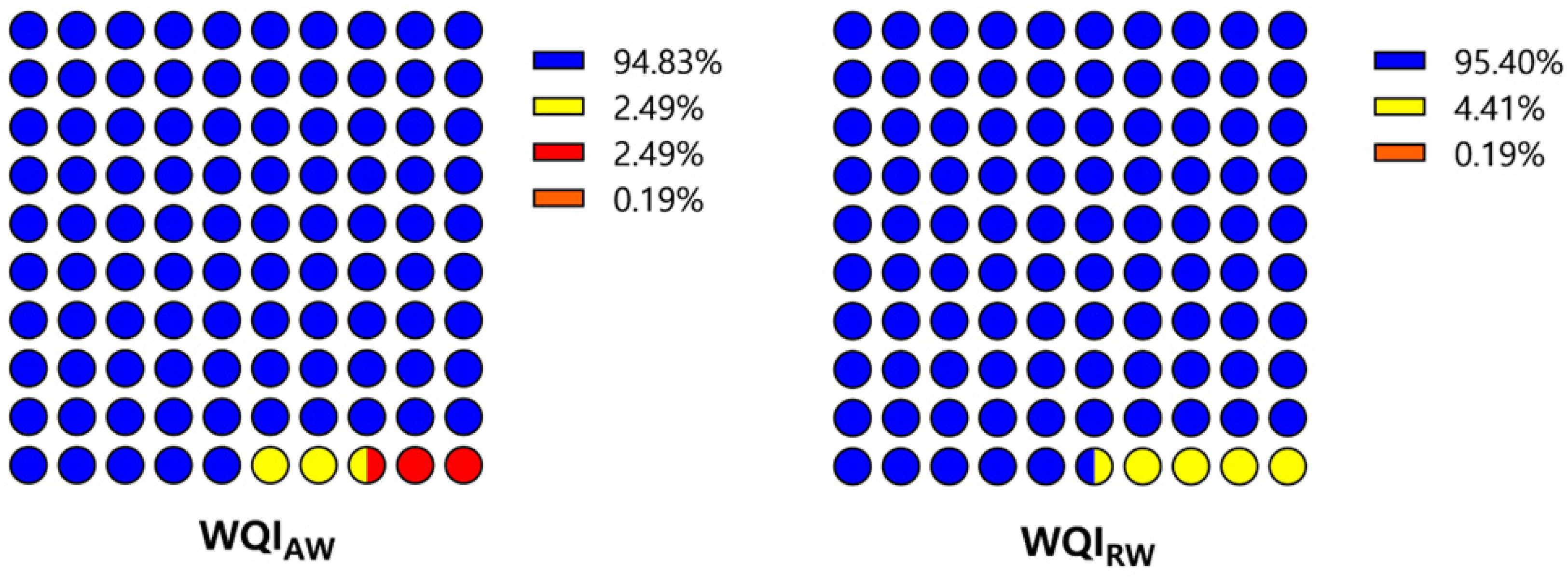
Figure 2 presents the water quality obtained through the modified WQIs.
The modified WQIs were shown to be comparable to the method that requires numerous field samplings and laboratory analyses. This was achieved by using sensor readings of electrical conductivity, dissolved oxygen, ammoniacal nitrogen, nitrate-nitrogen, pH, and turbidity, together with information on the current rain regime.
In both of the modified WQIs, there was a low percentage overestimation at more than one rating level (0.2%), which corresponded to only one observation. However, it was observed that WQIAW had a higher percentage underestimation (5.2%) compared to WQIRW, which underestimated only 1.3% of the time. These results suggest that online monitoring should not be used as the sole method for assessing water quality, and that sample collections and laboratory analyses should be conducted, not only when atypical measurements are observed, but also on a periodic basis, even at longer intervals [6,23,26].
The results obtained from the modified WQIs led to the generation of new fitting regression models for each WQI, which were aimed at reducing the errors associated with the modified indices. The resulting models were of the linear type, utilizing the scores obtained from WQIAW and WQIRW, and the scores obtained from WQICETESB, as presented in Table 8.
Both adjustment models obtained a good fit for the paired observations, as evidenced by R2 and R2adj values greater than 0.85. This indicates that the resulting equations can predict 85% of the variation observed in the WQICETESB scores, and that the WQIAW and WQIRW adjustment models can be utilized to minimize errors [28,31].
Pearson correlation analyses were conducted between the adjusted modified WQIs and WQICETESB, with the results presented in Table 9. The coefficients obtained were greater than 0.92, indicating a strong correlation [17,35] This suggests that the scores derived from the adjusted modified WQIs closely aligned with those obtained using WQICETESB.
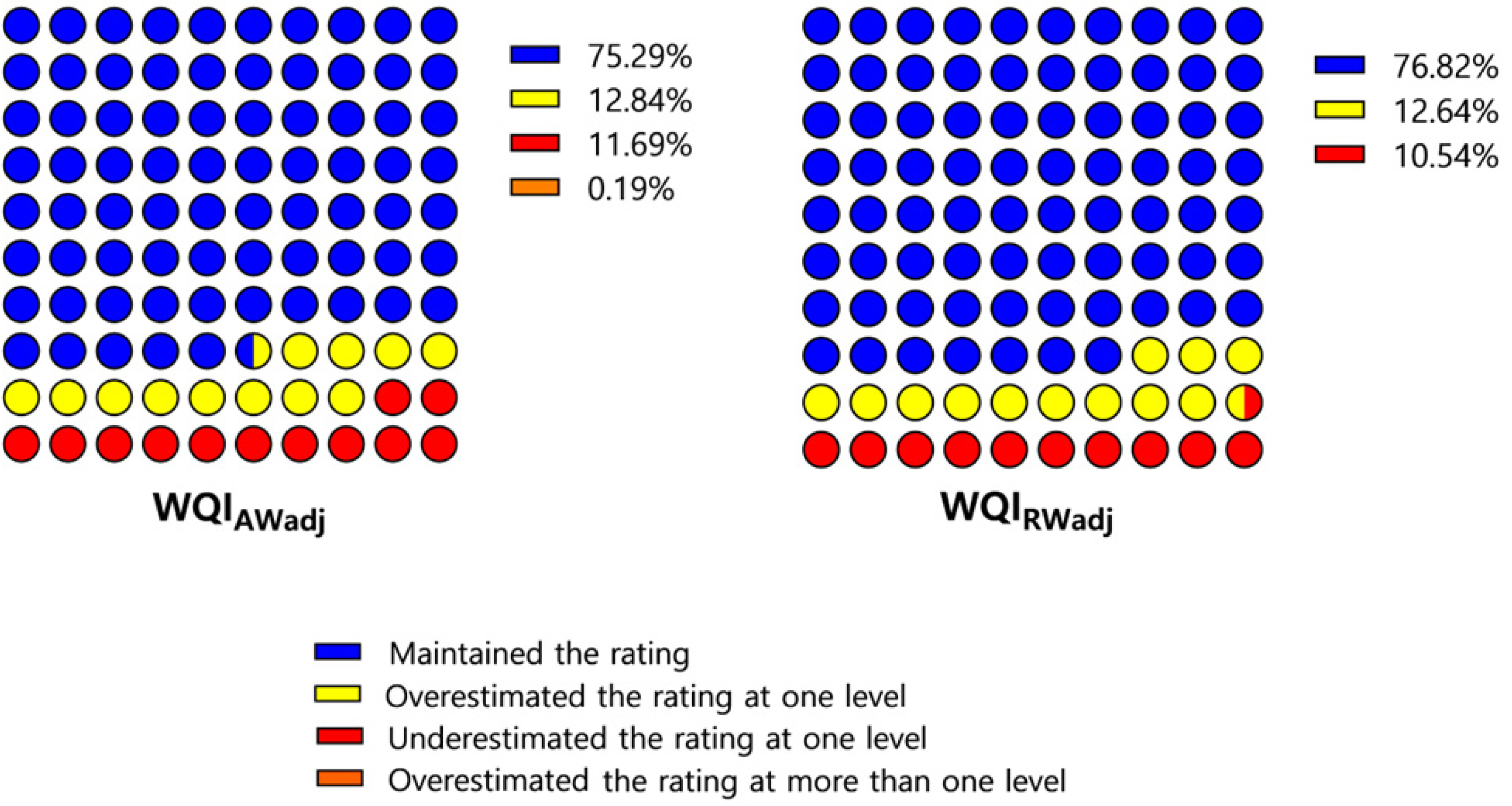
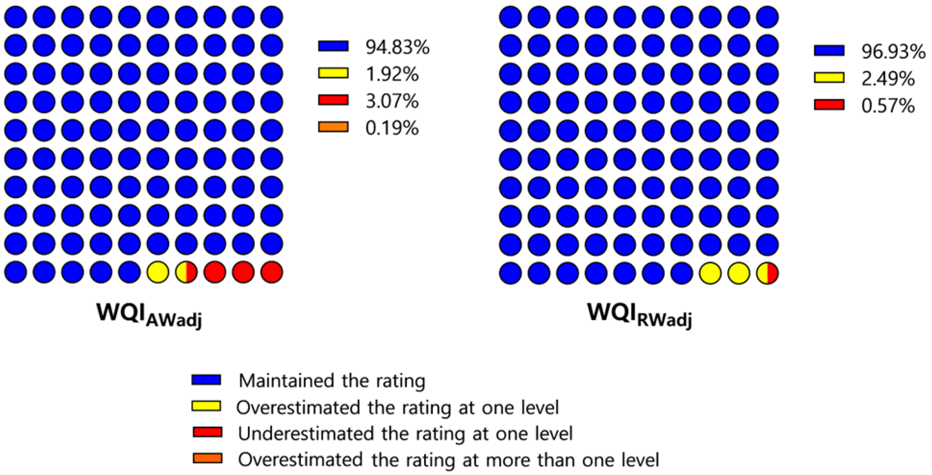
Figure 3 illustrates the proportion of correct and incorrect classification levels obtained by the adjusted modified WQIs, considering the intervals presented in Table 1. The success rate of WQIAWadj was slightly lower than that of WQIAW, while there was a 5.8% improvement in the success rate of WQIRW. It was also observed that for WQIRWadj, the adjustment could eliminate errors at more than one rating level, while, for WQIAWadj, it was not possible to eliminate these errors.
The adjustment equation for WQIAWadj decreased overestimation errors to 12.8%, while underestimation errors increased, resulting in an 11.6% underestimation rate in one rating level. A similar trend was observed for WQIRWadj, with a decrease in overestimation error (12.6%) compared to the original value (19.2%), and an increase in underestimation error (10.5%) compared to the original value (5.2%). Although the adjustments were unable to completely eliminate errors, WQIRWadj showed no errors in two or more rating levels of water quality, indicating robust results.

3.3. Comparison with Other Modified WQIs

In order to evaluate the performance of the modified WQIs in comparison to other water quality indices that also used easily measurable parameters, the indices proposed by Naveedullah et al. [4], Pesce and Wunderlin [23], and Moscuzza et al. [24] were compared. 
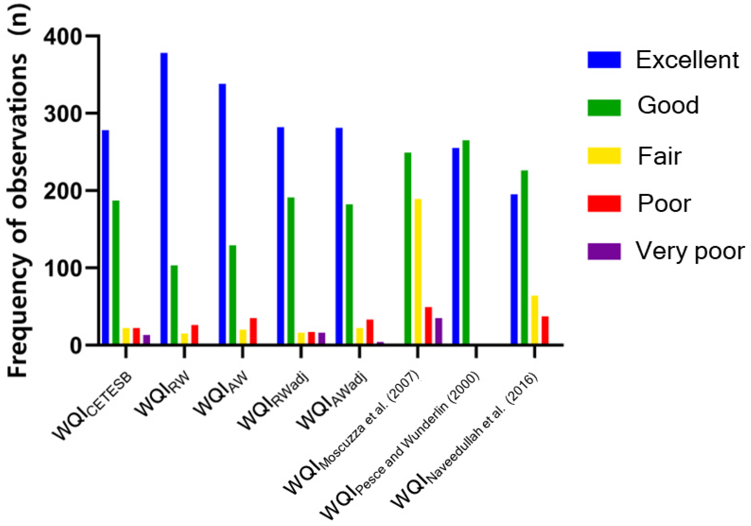
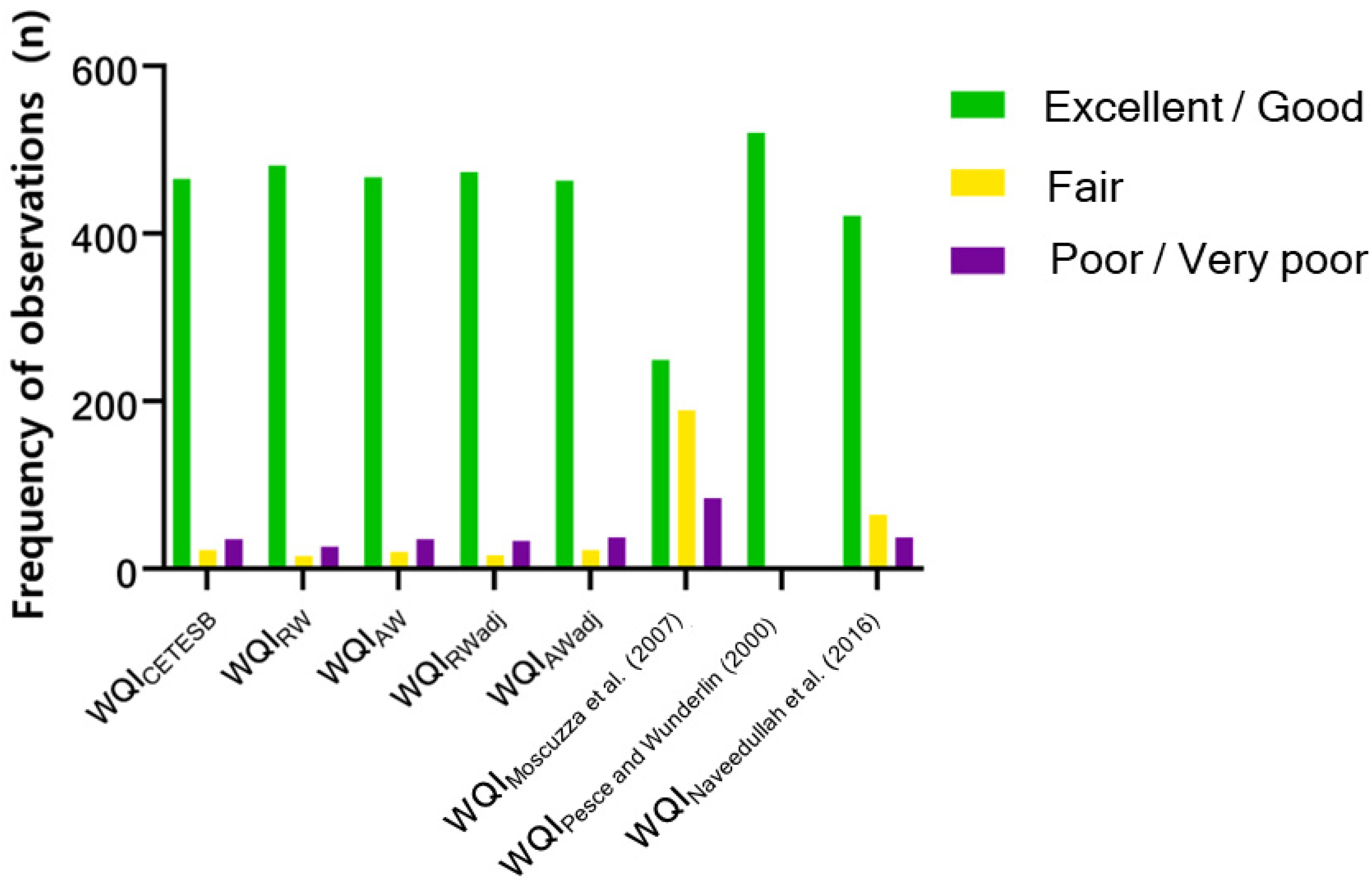
Figure 4 displays a comparison of the modified WQIs, the literature-based WQIs, and WQICETESB, using the water quality database of reservoirs in the state of São Paulo from 2018 to 2020.
WQIRW and WQIAW were found to frequently indicate ‘Excellent’ water quality, which can be attributed to the tendency to classify samples in the ‘Good’ quality level as ‘Excellent’. However, WQIRW exhibited overestimation of the ‘Poor’ rating levels and underestimation of the ‘Fair’ and ‘Very Poor’ rating levels (with the latter considered to be null), while WQIAW was more effective in indicating samples as ‘Fair’. Despite these differences, both WQIRW and WQIAW can provide useful information for decision-making in watershed management.
Upon observing the frequencies of each rating level of water quality indicated by WQIRWadj, it can be concluded that the adjustment was effective in correcting the errors associated with WQIRW and was successful in reducing the primary distortions identified earlier in the modified WQIRW. However, for WQIAWadj, despite the adjustment leading to fewer errors in the ‘Excellent’ rating level, it did not correctly identify any observations as ‘Very Poor’, which resulted in only four observations being classified as such. The adjustment also caused an overestimation of the ‘Poor’ category, although it did lead to an improvement in the success rate in the ‘Good’ and ‘Fair’ rating levels.
The frequencies of the observations obtained by the WQIs proposed in the literature differed from those obtained by the reference WQI. Moreover, when analyzing their success rate, the performance of these indices was inferior to those of the four modified WQIs proposed in this study. This can be elucidated by the absence of multiple dimensions of water quality, coupled with the fact that the indices were designed to cover the diverse situations, geographical locations, and inherent attributes of distinct water bodies.

3.4. Simplified Classification of Water Quality

Table 10 presents a simplified classification, which considers that water classified as ‘Excellent/Good’ and ‘Poor/Very Poor’ overlap each other mainly with regard to the collection/supply and treatment of water for public/municipal purposes [6].
Figure 5 shows the success and error rates of the proposed WQIS when the simplified classification is used.
The results of the WQIs modified with a simplified scheme indicate a notable achievement in terms of the success rate. The employment of the simplified classification scheme resulted in a noteworthy reduction in the parcel of overestimation for rating level errors, as evidenced by the decrease in the previously observed range of overestimation errors from 12.64% to 27.39% to a narrower range of 4.41% to 1.92%. In addition, the use of the simplified approach led to a similar reduction in the underestimation error of one rating level, with a reduction of up to 9.97 percentage points noted, as seen with WQIRWadj.
WQIRWadj exhibited superior performance compared to the other modified WQIs indicating the correct classification (96.9%), without errors at more than one level rating. It also had the lowest error rate of underestimation (0.6%) and a low rate of overestimation (2.5%).
In order to compare the performance of the proposed WQIs with other WQIs proposed in the literature, simplified classification was used, and the frequencies of each WQI indicated for each category are plotted in Figure 6. It was observed that the modified WQIs performed similarly to each other and the reference WQI, indicating a good level of agreement. However, the WQIs proposed in the literature exhibited poor performance, with the WQI proposed by Naveedullah et al. [4] being the one that exhibited the best performance among them.

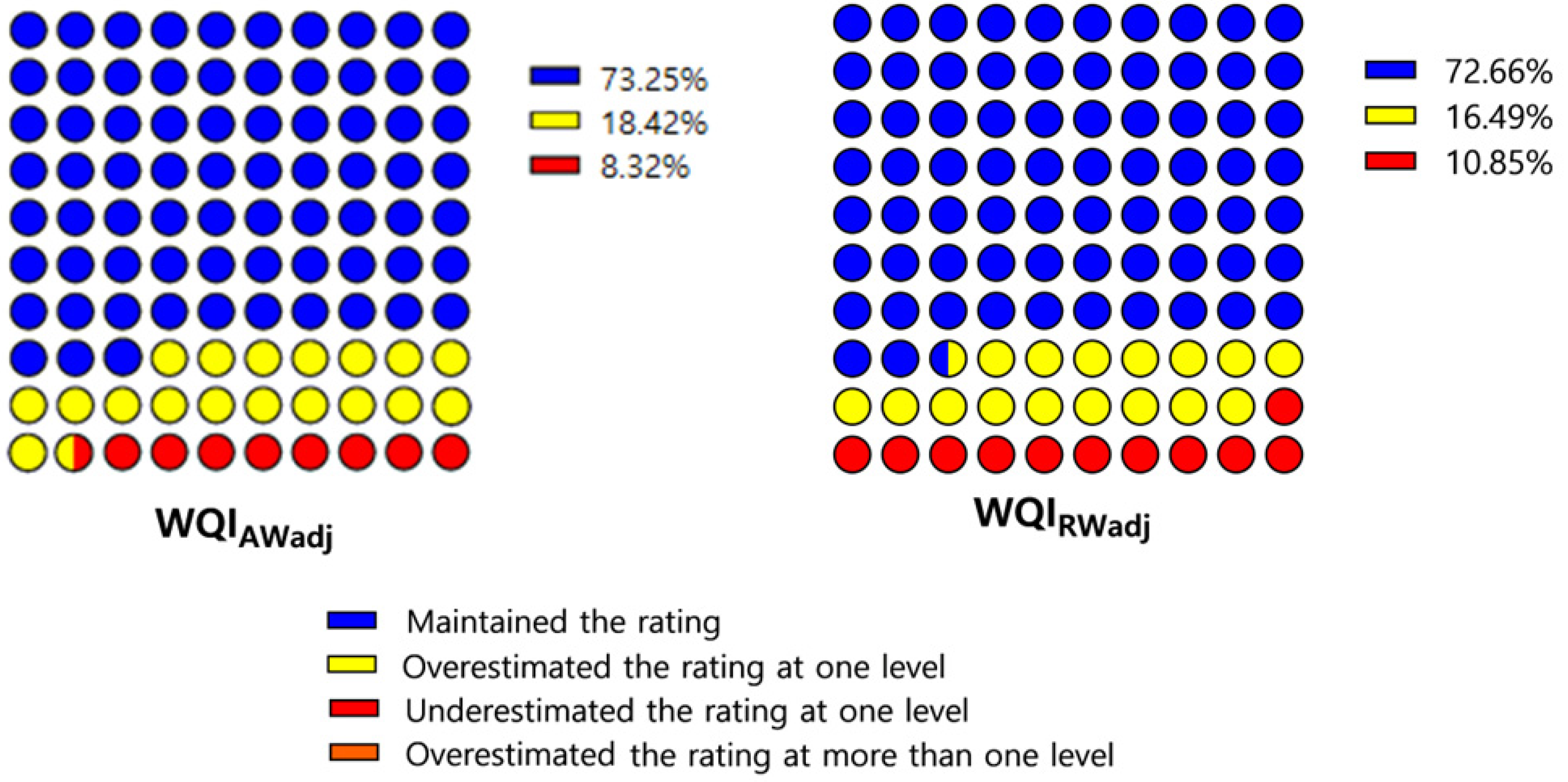
3.5. Validating the Modified Water Quality Indices

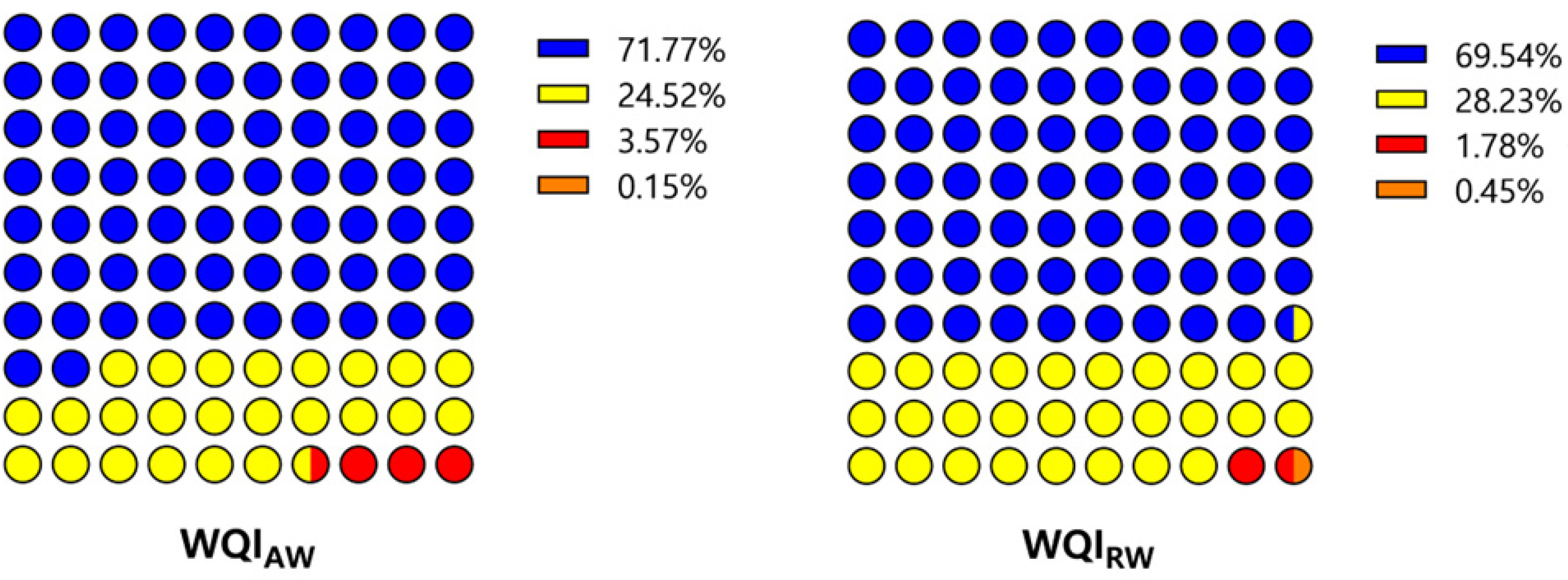
During the validation step of the modified WQIS, a database of water quality from reservoirs in the state of São Paulo was used, covering a period prior to that used during the modeling step (2003 to 2007). The results of the modified WQIs in comparison to WQICETESB are presented in Figure 7.
All of the compared indices had a success rate of approximately 70%, with WQIRW having the lowest performance at 69.54%. Conversely, WQIAWadj had the highest success rate at 73.25%. These success rates were similar to the values obtained during the construction of the modified WQIs. Furthermore, the adjusted indices were able to eliminate errors at more than one rating level during the validation step. WQIRWadj stands out as it succeeded in eliminating errors at more than one rating level in both the construction and validation steps, and presented good success rates (76.82% and 72.66%, respectively) throughout the present study.
Additionally, it is important to note that WQIRWadj continued to exhibit a 10% rate of overestimation at one rating level, while also displaying a portion of underestimation at one rating level, which reached 16.5%. Furthermore, WQIAWadj showed a decrease in the overestimation error to 8.3% at one rating level, but an increase in the underestimation error to 18.4% at one rating level, when compared to the results obtained during the construction step of the modified WQI.
Based on the results obtained in the present study, WQIRWadj was found to be the most effective modified WQI. During the construction phase, it demonstrated the highest rate of correct classification, with no errors occurring at more than one rating level. In the validation phase, it continued to perform well, with no errors occurring at more than one rating level and achieving a low overestimation error percentage, resulting in a high success rate.
To assess the performance of modified indices relative to WQICETESB, a correlation analysis was conducted between the scores obtained by modified indices proposed in other studies [4,23,24] and those obtained by modified indices proposed in this study. Table 11 presents the correlation values obtained, allowing for a comparison of the performance of the different modified WQIs using WQICETESB as a reference. Thus, it is possible to verify that the indices, both modified and adjusted modified, proposed in the present study presented very strong correlations (>0.9279) with the values obtained by the CETESB water quality assessment methodology. In contrast, we observed that the index modified proposed by Pesce and Wunderlin [23] failed to obtain results similar to those obtained by WQICETESB. The modified indices proposed by Naveedullah et al. [4] and by Moscuzza et al. [24] had better performances, showing strong (0.7467) and moderate (0.6511) correlations, respectively.
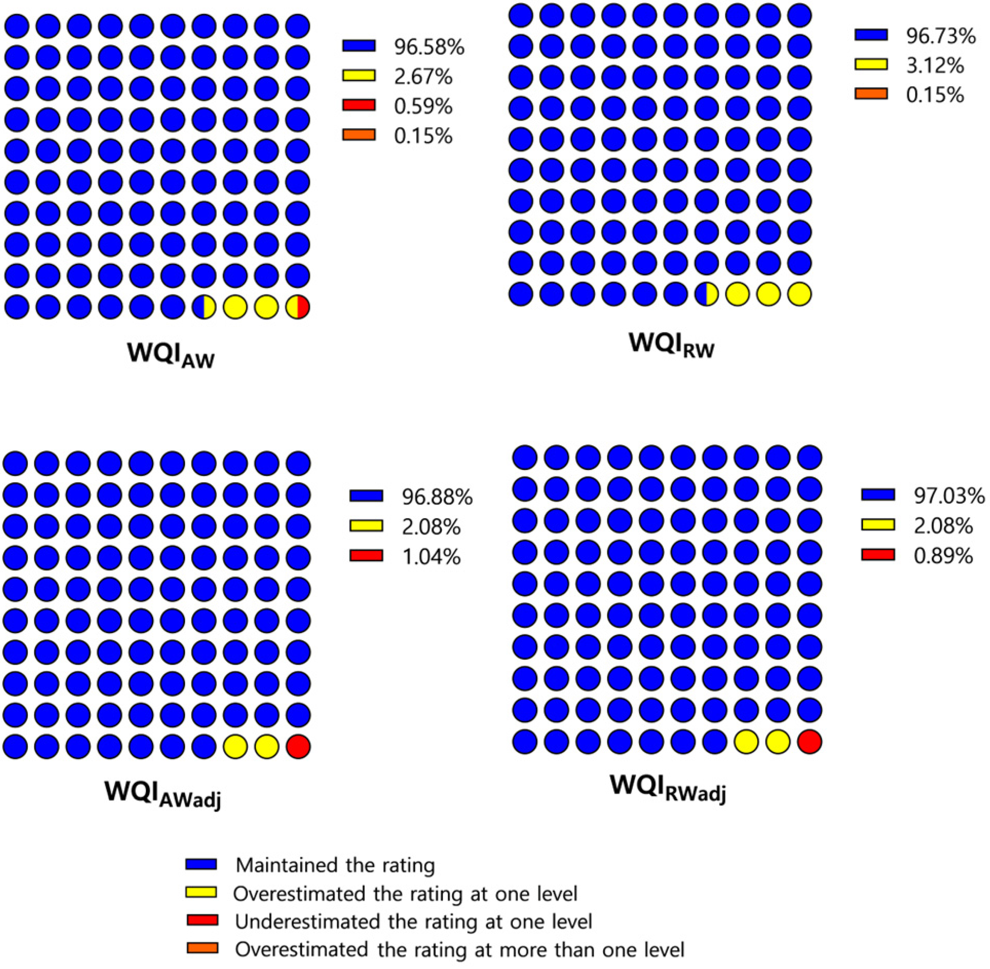
The simplified classification scheme presented in Table 10 was also used in the validation step to evaluate the performance of modified WQIs when using fewer rating levels. Figure 8 shows the results achieved in the step for each of the modified WQIs.
It can be observed that all the WQIs had a high success rate, around 96%, in the validation step. However, the error at more than one rating level remained in the modified WQIs. This type of error is inadmissible because it indicates a very different water quality from the reality, which can lead to poor decision-making. It is noteworthy that the adjustment was able to eliminate this type of error in both the strategies of attributed and redistributed weights. Even with the WQIs adjustment, errors in indicating the wrong status of the water quality still occurred, but these errors were reduced. In most cases, the WQIs correctly adjusted the water quality rating or indicated a worse rating level than it really was. Thus, the results validated the efficiency of the modified adjusted WQIs when applying a scheme of simplified classification. In general, WQIRWadj stood out for having the smallest portion of underestimated error and a higher success rate.
The modified WQIs constructed in this study are capable of indicating water quality classifications for other sets of data besides the databases used in their modeling and construction, as evidenced by the validation step. The performance of WQIRWadj should also be highlighted, as this WQI presented no errors at more than one rating level, a lower overestimation error rate, and a very high success rate. WQIRWadj can be renamed as WQISOL to make it more accessible and promote its dissemination for use in monitoring reservoirs. The letter S indicates the locality for which it was idealized, i.e., the State of São Paulo, and the letters OL denote the methodology of determining the status of water quality, which is an online determination method. Therefore, the initials form the word “SOL,” which means 
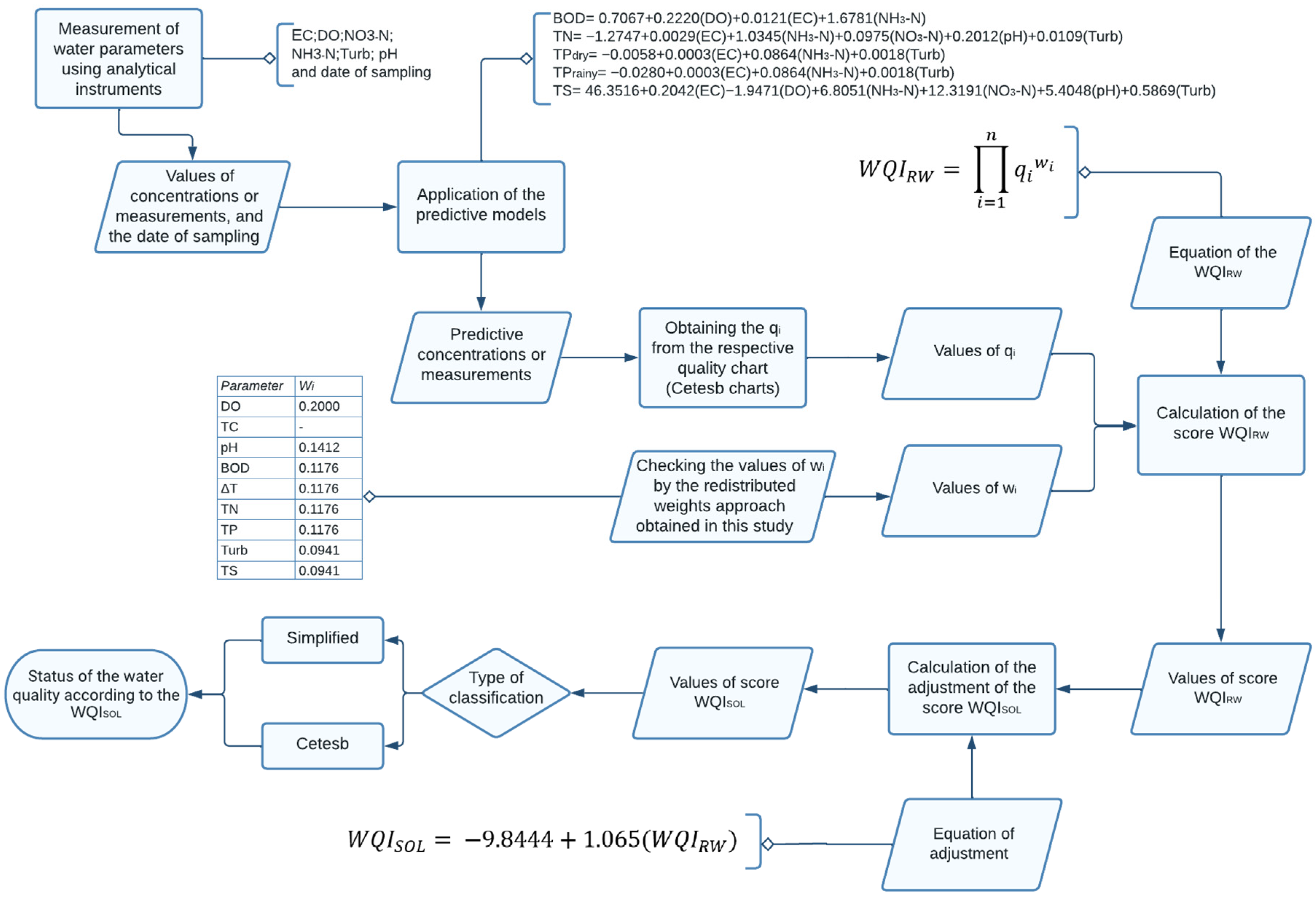
sun in Portuguese, giving it an even more friendly connotation. To encourage the application of WQISOL in monitoring reservoirs, a schematic diagram for the calculation of the modified IQA was prepared to facilitate the application of the methodology proposed in the present study, which can be found in Figure 9.
The process for calculating WQISOL, as shown in Figure 9, involves several steps. First, measurement data obtained from sensors are used as inputs for the prediction regression models, which generate predicted values for relevant parameters. These predicted values are then used to calculate WQIRW. The resulting output value is then passed through the adjustment equation. Based on the resulting value, the appropriate classification method can be selected. To help users understand the process, explanatory notes, such as equations or weighted values, have been included in the diagram, denoted by a line and an empty diamond with a parenthesis. As a result, the diagram can serve as a guide for using WQISOL to monitor reservoirs.

4. Conclusions

The construction of predictive models and the composition of WQISOL (WQIRWadj) have enabled the reliable and continuous determination of the water quality in reservoirs in the Brazilian state of São Paulo without the need for costly and time-consuming sampling campaigns or laboratory analyses. This allows for efficient monitoring and management of water resources, ensuring that water quality is maintained at acceptable levels.
The study found that the method of weighted redistribution together with the regression adjustment (WQISOL), was the best option among the modified WQIs. This is because it showed a high level of similarity to WQICETESB, and demonstrated a more uniform and superior performance compared to other modified WQIs. WQISOL stands out as it succeeded in eliminating errors at more than one rating level in both the construction and validation steps, and presented good success rates (76.82% and 72.66%, respectively). Moreover, the success rate was equal to 97% in the validation step for a simplified (three-range) classification system.
WQISOL offers the potential for more sustainable and economical real-time monitoring of water quality as it eliminates the need for a significant portion of water sampling and analysis. Moreover, by making the WQISOL results available for public consultation online through interactive maps, it can increase environmental awareness and promote social responsibility among surrounding communities. The proposed simplified classification demonstrated its potential as a viable option for effective watershed management.
To ensure accurate water quality monitoring, it is recommended to continue using the monitoring methods, albeit at a possible reduced frequency, to avoid misinterpreting water quality data. In order to improve WQISOL and reduce classification errors, future studies should focus on the development of a predictive model using parameters that can be easily measured by analytical instruments and can efficiently determine the counts of E. coli or thermotolerant coliforms. This model could then be integrated into the WQISOL framework. The use of tools such as artificial intelligence could help in the development of this model.
Additionally, it is suggested that WQISOL be tested in reservoirs located in other regions with similar conditions and high urbanization levels to verify its effectiveness in those regions. Finally, it is recommended to explore the application of WQISOL in other types of waterbodies to determine its potential use beyond reservoirs.

Author Contributions

Conceptualization, P.L.C.S. and A.C.B.; methodology, P.L.C.S. and A.C.B.; formal analysis, P.L.C.S. and A.C.B.; investigation, P.L.C.S.; resources, A.C.B.; data curation, P.L.C.S.; writing—original draft preparation, P.L.C.S. and L.S.L.; writing—review and editing, P.L.C.S., A.C.B., L.S.L. and A.P.R.; supervision, A.C.B. and A.P.R.; project administration, P.L.C.S. and A.C.B.; funding acquisition, P.L.C.S. All authors have read and agreed to the published version of the manuscript.

Funding

This study was funded in part by the Coordination for the Improvement of Higher Education Personnel (CAPES Finance Code 001).

Data Availability Statement

Not applicable.

Conflicts of Interest

The authors declare no conflict of interest.

References

  1. Boretti, A.; Rosa, L. Reassessing the projections of the World Water Development Report. NPJ Clean Water 2019, 2, 15. [Google Scholar] [CrossRef]
  2. Simeonov, V.; Stratis, J.; Samara, C.; Zachariadis, G.; Voutsa, D.; Anthemidis, A.; Sofoniou, M.; Kouimtzis, T. Assessment of the surface water quality in Northern Greece. Water Res. 2003, 37, 4119–4124. [Google Scholar] [CrossRef]
  3. Sánchez, E.; Colmenarejo, M.F.; Vicente, J.; Rubio, A.; García, M.G.; Travieso, L.; Borja, R. Use of the water quality index and dissolved oxygen deficit as simple indicators of watersheds pollution. Ecol. Indic. 2007, 7, 315–328. [Google Scholar] [CrossRef]
  4. Naveedullah, N.; Hashmi, M.Z.; Yu, C.; Shen, C.; Muhammad, N.; Shen, H.; Chen, Y. Water Quality Characterization of the Siling Reservoir (Zhejiang, China) Using Water Quality Index. CLEAN—Soil Air Water 2016, 44, 553–562. [Google Scholar] [CrossRef]
  5. Tirkey, P.; Bhattacharya, T.; Chakraborty, S. Water Quality Indices-Important Tools for Water Quality Assessment: A Review. Int. J. Adv. Chem. (IJAC) 2015, 1, 15–29. [Google Scholar]
  6. Oliveira, A.R.M. Desenvolvimento de Índices de Qualidade da Água com Número Reduzido de Parâmetros. Ph.D. Thesis, Universidade Federal de Viçosa, Viçosa, Brazil, 2017. [Google Scholar]
  7. Jeronimo, C.E.D.M.; Souza, F.R.S. Determinação do Índice de Qualidade da Água da Lagoa de Extremoz-RN: Série Temporal e Correlação a Indices Pluviométricos. Rev. Eletrônica Gestão Educ. Tecnol. Ambient. 2013, 10, 2219–2232. [Google Scholar] [CrossRef]
  8. Li, P.; Qian, H.; Wu, J. Groundwater Quality Assessment Based on Improved Water Quality Index in Pengyang County, Ningxia, Northwest China. J. Chem. 2010, 7, S210–S216. [Google Scholar] [CrossRef]
  9. Yang, Y.; Li, P.; Elumalai, V.; Ning, J.; Xu, F.; Mu, D. Groundwater Quality Assessment Using EWQI With Updated Water Quality Classification Criteria: A Case Study in and Around Zhouzhi County, Guanzhong Basin (China). Expo. Health 2022, 1–16. [Google Scholar] [CrossRef]
  10. Wu, J.; Zhang, Y.; Zhou, H. Groundwater chemistry and groundwater quality index incorporating health risk weighting in Dingbian County, Ordos basin of northwest China. Geochemistry 2020, 80, 125607. [Google Scholar] [CrossRef]
  11. Nsabimana, A.; Li, P. Hydrogeochemical characterization and appraisal of groundwater quality for industrial purpose using a novel industrial water quality index (IndWQI) in the Guanzhong Basin, China. Geochemistry 2023, 83, 125922. [Google Scholar] [CrossRef]
  12. Katyal, D. Water Quality Indices Used for Surface Water Vulnerability Assessment. Int. J. Environ. Sci. 2011, 2, 154–173. [Google Scholar]
  13. Goher, M.E.; Hassan, A.M.; Abdel-Moniem, I.A.; Fahmy, A.H.; El-Sayed, S.M. Evaluation of surface water quality and heavy metal indices of Ismailia Canal, Nile River, Egypt. Egypt. J. Aquat. Res. 2014, 40, 225–233. [Google Scholar] [CrossRef]
  14. APHA. Standard Methods for the Examination of Water and Wastewater, 23rd ed.; American Public Health Association: Washington, DC, USA, 2017. [Google Scholar]
  15. CETESB. Monitoramento de Escherichia Coli e Coliformes Termotolerantes em Pontos da Rede de Avaliação da Qualidade de Águas Interiores do Estado de São Paulo; CETESB: Bauru, Brazil, 2008.
  16. Hachich, E.M.; Di Bari, M.; Christ, A.P.G.; Lamparelli, C.C.; Ramos, S.S.; Sato, M.I.Z. Comparison of thermotolerant coliforms and Escherichia coli densities in freshwater bodies. Braz. J. Microbiol. 2012, 43, 675–681. [Google Scholar] [CrossRef]
  17. Spearman, C. The Proof and Measurement of Association between Two Things. In Studies in Individual Differences: The Search for Intelligence; Appleton-Century-Crofts: East Norwalk, CT, USA, 1961; pp. 45–58. [Google Scholar]
  18. Magalhães, S.R. Teste Para Verificar a Igualdade de Modelos de Regressão e uma Aplicação na Área Médica. E-Xacta 2009, 2, 34–41. [Google Scholar] [CrossRef]
  19. Hoffmann, R. Análise de Regressão: Uma Introdução à Econometria; Hucitec: Piracicaba, Brazil, 2016. [Google Scholar]
  20. Brooks, C. Introductory Econometrics for Finance, 2nd ed.; Cambridge University Press: Cambridge, UK, 2008. [Google Scholar]
  21. Nash, J.E.; Sutcliffe, J.V. River flow forecasting through conceptual models part I—A discussion of principles. J. Hydrol. 1970, 10, 282–290. [Google Scholar] [CrossRef]
  22. CETESB. Qualidade das Águas Interiores no Estado de São Paulo (Anexos). Available online: www.cetesb.sp.gov.br/aguas-interiores/wp-content/uploads/sites/12/2013/11/02.pdf (accessed on 6 May 2023).
  23. Pesce, S.; Wunderlin, D.A. Use of water quality indices to verify the impact of Córdoba City (Argentina) on Suquía River. Water Res. 2000, 34, 2915–2926. [Google Scholar] [CrossRef]
  24. Moscuzza, C.; Volpedo, A.V.; Ojeda, C.; Cirell, A.F. Water Quality Index as a Tool for River Assessment in Agricultural Areas in the Pampean Plains of Argentina. J. Urban Environ. Eng. 2007, 1, 18–25. [Google Scholar] [CrossRef]
  25. Von Sperling, M. Wastewater Characteristics, Treatment and Disposal; IWA Publishing: London, UK, 2007. [Google Scholar] [CrossRef]
  26. Rose, C.; Parker, A.; Jefferson, B.; Cartmell, E. The Characterization of Feces and Urine: A Review of the Literature to Inform Advanced Treatment Technology. Crit. Rev. Environ. Sci. Technol. 2015, 45, 1827–1879. [Google Scholar] [CrossRef]
  27. Walton, N. Electrical Conductivity and Total Dissolved Solids—What is Their Precise Relationship? Desalination 1989, 72, 275–292. [Google Scholar] [CrossRef]
  28. Barros Neto, B.; Scarminio, I.S.; Bruns, R.E. Como Fazer Experimentos: Pesquisa e Desenvolvimento na Ciência e na Indústria; Editora da Unicamp: Campinas, Brazil, 2001; ISBN 8526805444. [Google Scholar]
  29. Eryani, I.G.A.P.; Jayantari, M.W.; Wijaya, I.K.M. Sensitivity Analysis in Parameter Calibration of the WEAP Model for Integrated Water Resources Management in Unda Watershed. Civ. Eng. Arch. 2022, 10, 455–469. [Google Scholar] [CrossRef]
  30. Kusari, L. Regression Model as a Tool to Predict Concentrations of Total Suspended Solids in Rivers. EQA—Int. J. Environ. Qual. 2017, 23, 35–42. [Google Scholar] [CrossRef]
  31. Cea, L.; Bermúdez, M.; Puertas, J. Uncertainty and sensitivity analysis of a depth-averaged water quality model for evaluation of Escherichia Coli concentration in shallow estuaries. Environ. Model. Softw. 2011, 26, 1526–1539. [Google Scholar] [CrossRef]
  32. Mohammed, H.; Tveten, A.-K.; Seidu, R. Modelling the impact of climate change on flow and E. coli concentration in the catchment of an ungauged drinking water source in Norway. J. Hydrol. 2019, 573, 676–687. [Google Scholar] [CrossRef]
  33. Palazón, A.; López, I.; Aragonés, L.; Villacampa, Y.; Navarro-González, F. Modelling of Escherichia coli concentrations in bathing water at microtidal coasts. Sci. Total Environ. 2017, 593–594, 173–181. [Google Scholar] [CrossRef] [PubMed]
  34. Wang, J.; Deng, Z. Modeling and predicting fecal coliform bacteria levels in oyster harvest waters along Louisiana Gulf coast. Ecol. Indic. 2019, 101, 212–220. [Google Scholar] [CrossRef]
  35. Srivastava, G.; Kumar, P. Water Quality Index with Missing Parameters. IJRET Int. J. Res. Eng. Technol. 2013, 2, 609–614. [Google Scholar]
Figure 1. Map of the region of São Paulo state, highlighting the reservoirs included in the study.
Hydrology 10 00115 g001
Figure 2. Percentage of observations obtained by the modified WQI using assigned weights (WQIAW) and redistributed weights (WQIRW) compared to the water quality classification of WQICETESB.
Hydrology 10 00115 g002
Figure 3. Percentage of observations obtained by the modified WQI using adjusted assigned weights (WQIPAaj) and redistributed weights (WQIRWadj) compared to the water quality classification of WQICETESB.
Hydrology 10 00115 g003
Figure 4. Frequency of observations for each rating level: WQICETESB, modified WQI using assigned weights (WQIAW), adjusted modified WQI using assigned weights (WQIAWadj), modified WQI using redistributed weights (WQIRW), adjusted modified WQI using redistributed weights (WQIRWadj), and previous modified WQIs presented in literature. Data from São Paulo reservois (2018 to 2020).
Hydrology 10 00115 g004
Figure 5. Percentage of observations obtained by the modified WQI using assigned weights (WQIAW), adjusted modified WQI using assigned weights (WQIAWadj), modified WQI using redistributed weights (WQIRW), and adjusted modified WQI with redistributed weights (WQIRWadj) compared to the water quality classification of WQICETESB, using the simplified classification.
Hydrology 10 00115 g005aHydrology 10 00115 g005b
Figure 6. Frequency of observations for each class: WQICETESB, modified WQI using assigned weights (WQIAW), adjusted modified WQI using assigned weights (WQIAWadj), modified WQI using redistributed weights (WQIRW), adjusted modified WQI using redistributed weights (WQIRWadj), WQI proposed by Moscuzza et al. [24], WQI proposed by Pesce and Wunderlin [23], and WQI proposed by Naveedullah et al. [4], using the simplified classification.
Hydrology 10 00115 g006
Figure 7. Percentage of observations by the modified WQI using assigned weights (WQIAW), adjusted modified WQI with assigned weights (WQIAWadj), modified WQI with redistributed weights (WQIRW), and adjusted modified WQI with redistributed weights (WQIRWadj), compared to the water quality classification of WQICETESB.
Hydrology 10 00115 g007aHydrology 10 00115 g007b
Figure 8. Percentage of observations by the modified WQI using assigned weights (WQIAW), ad-justed modified WQI with assigned weights (WQIAWadj), modified WQI with redistributed weights (WQIRW), and adjusted modified WQI with redistributed weights (WQIRWadj), compared to the water quality classification of WQICETESB, using the simplified classification.
Hydrology 10 00115 g008
Figure 9. A schematic diagram illustrating the calculation process for WQISOL.
Hydrology 10 00115 g009
Table 1. Classification of water quality by WQICETESB.
CategoryScoreColor
Excellent79 < WQI ≤ 100
Good51 < WQI ≤ 79
Fair36 < WQI ≤ 51
Poor19 < WQI ≤ 36
Very PoorWQI ≤ 19
Source: CETESB [15,22].
Table 2. Spearman’s correlation (ρ) between the independent and dependent parameters.
ECDONH3-NNO3-NpHTTurb
BODr0.4141−0.13220.49820.06050.055−0.0780.4643
p-value<0.0001<0.0001<0.00010.00370.00830.0002<0.0001
TPr0.5181−0.27630.46260.1555−0.0143−0.05880.5265
p-value<0.0001<0.0001<0.0001<0.00010.4898 ns0.0052<0.0001
TNr0.7041−0.23930.53430.45530.1474−0.02070.4201
p-value<0.0001<0.0001<0.0001<0.0001<0.00010.3207 ns<0.0001
TSr0.728−0.24610.3810.32840.14790.03340.3909
p-value<0.0001<0.0001<0.0001<0.0001<0.00010.1086 ns<0.0001
Table 3. Predictive models for the values of the WQI using variables that can be measured by probes.
Equation
BOD = 0.7067 + 0.2220(DO) + 0.0121(EC) + 1.6781(NH3-N)
TPdry = −0.0058 + 0.0003(EC) + 0.0864(NH3-N) + 0.0018(Turb)
TPrainy = −0.0280 + 0.0003(EC) + 0.0864(NH3-N) + 0.0018(Turb)
TN = −1.27447 + 0.0029(EC) + 1.0345(NH3-N) + 0.09748(NO3-N) + 0.2012(pH) + 0.0109(Turb)
TS = 46.3516 + 0.2042(EC) − 1.9471(DO) + 6.8051(NH3-N) + 12.3191(NO3-N) + 5.4058(pH) + 0.5869(Turb)
Table 4. Coefficients of determination obtained when adjusting the models.
ParameterAdjustment
R2R2adj
BOD0.71410.7137
TP(dry and rainy)0.83120.8309
TN0.92390.9237
TS0.78430.7837
Table 5. Coefficients of determination, Pearson correlation (r), and Nash–Sutcliffe efficiency coefficient (NSE) obtained when validating the regression models.
ParameterR2R2adjr(Pearson)NSE
BOD0.71330.71280.83980.6758
TP0.90530.90510.95150.8951
TN0.95520.95510.99480.9495
TS0.83470.83440.91360.8290
Table 6. Weights (wi) of the parameters for calculating the water quality indices (WQI) modified with assigned weights (WQIAW), redistributed weights (WQIRW), and original weights (WQICETESB).
ParameterWQIAWWQIRWWQICETESB
DO0.25000.20000.1700
TC--0.1500
pH0.18000.14120.1200
BOD *0.08000.11760.1000
ΔT0.08000.11760.1000
TN *0.08000.11760.1000
TP *0.08000.11760.1000
Turb0.20000.09410.0800
TS *0.05000.09410.0800
* Parameters determined indirectly using regressions obtained in this study.
Table 7. Pearson correlation coefficients (r) for WQIAW and WQIRW in relation to WQICETESB, obtained with the set of water quality data for reservoirs in the state of São Paulo, from 2018 to 2020.
Indexr(Pearson)p-Value
WQIAW0.9285<0.001
WQIRW0.9291<0.001
Table 8. Regression models adjusted for WQIAW and WQIRW.
EquationR2R2adj
WQIAWadj = 0.9783 (WQIAW) − 1.56030.85650.8563
WQIRWadj = 1.0656 (WQIRW) − 9.89440.85430.8540
WQIAWadj and WQIRWadj were obtained of regressions models between the scores of modified WQIs versus WQICETESB.
Table 9. Pearson correlation coefficients (r) for WQIWAadj and WQIRWadj in relation to WQICETESB, for the set of water quality data for reservoirs in the state of São Paulo, from 2018 to 2020.
Indexrp-Value
WQIAWadj0.9285<0.001
WQIRWadj0.9285<0.001
Table 10. Proposed simplified classification of water quality, with the CETESB classification [6].
CETESBSIMPLIFIED
CategoryRangeColorCategoryRangeColor
Excellent79 < IQA ≤ 100 Excellent/Good51 < IQA ≤ 100
Good51 < IQA ≤ 79
Fair36 < IQA ≤ 51 Fair36 < IQA ≤ 51
Poor19 < IQA ≤ 36 Poor/Very PoorIQA ≤ 36
Very PoorIQA ≤ 19
Table 11. Pearson correlation coefficients (r) for the modified WQI using assigned weights (WQIAW), adjusted modified WQI using assigned weights (WQIAWadj), modified WQI with redistributed weights (WQIRW), adjusted modified WQI with redistributed weights (WQIRWadj), WQI proposed by Moscuzza et al. [24], WQI proposed by Pesce and Wunderlin [23], and WQI proposed by Naveedullah et al. [4] in relation to WQICETESB obtained with the set of water quality data for reservoirs in the state of São Paulo, from 2003 to 2007.
Indexrp-Value
WQIAW0.9379<0.001
WQIRW0.9379<0.001
WQIAWadj0.9279<0.001
WQIRWadj0.9353<0.001
Moscuzza et al. [23]0.6511<0.001
Pesce and Wunderlin [24]0.3186<0.001
Naveedullah et al. [4]0.7467<0.001
Disclaimer/Publisher’s Note: The statements, opinions and data contained in all publications are solely those of the individual author(s) and contributor(s) and not of MDPI and/or the editor(s). MDPI and/or the editor(s) disclaim responsibility for any injury to people or property resulting from any ideas, methods, instructions or products referred to in the content.

