
Reservoir Ice Conditions from Multi-Sensor Remote Sensing and ERA5-Land: The Manicouagan Hydroelectric Reservoir Case Study

Département de Génie Civil et de Génie du Bâtiment, Université de Sherbrooke, Sherbrooke, QC J1K 2R1, Canada
*
Author to whom correspondence should be addressed.
Hydrology 2023, 10(5), 108; https://doi.org/10.3390/hydrology10050108
Submission received: 29 March 2023
/
Revised: 14 April 2023
/
Accepted: 5 May 2023
/
Published: 11 May 2023
Abstract
:Reservoir ice can have an important impact on the watershed scale and influence hydraulic operations. On the other hand, hydropower generation can also impact the ice regime. In this study, multi-source satellite and ERA5-land data are used to evaluate ice conditions. Specifically, ice-controlling variables (temperature, water levels), ice regime (cover/deformation, thickness) and their interrelations are assessed for a 5-year period from 2017 to 2021. The methodology is applied to the Manicouagan reservoir, one of the largest hydropower reservoirs in Quebec, Canada. The satellite-based land surface temperatures (LSTs) suggest that winter 2021 was the hottest one. Overall, MODIS and Landsat LSTs agree with the ERA5-land temperatures. Ice backscatter from Sentinel-1 indicates that, in general, the reservoir is completely covered by ice from January to March. A correlation of 0.6 and 0.8 is observed between C- and Ku-band Synthetic Aperture Radar (SAR) signal and ice thickness, respectively. Important ice changes inferred from Differential Interferometric SAR (D-InSAR) occur approximately at the position where the largest ERA5-land ice thickness differences are observed. Winter water levels are also evaluated using satellite altimetric data to verify their influence on the ice dynamics. They show a decreasing tendency as the winter advances.
1. Introduction
Ice is a key element of high-latitude landscapes and has been widely considered a climate change indicator (e.g., [1]). The presence and characteristics of ice in human-made or natural water bodies need to be evaluated for a comprehensive understanding of the hydro–ecological system’s dynamics at these locations. In the case of reservoirs, hydropower operations at high latitudes are reported to be potentially influenced by the presence of ice, which can cause a loss of energy, particularly during the freeze-up period, and also could lead to safety problems [2]. On the other hand, hydropower regulations can notably modify ice regime [3].
Despite its importance from environmental and socioeconomic viewpoints, investigations of ice in lakes, rivers and reservoirs are usually scarce compared to environmental studies on the ice-off seasons because of the usual remoteness of the sites and challenges for acquiring in situ measurements. The advent of satellite technology opened new doors for the investigation of landscape elements where local observations are scarce or difficult to obtain. The long-term monitoring of ice dynamics in a context of climate change is possible thanks to a large archive of remote sensing and in-situ observations.
Some remote sensing data and techniques have been used in the last few decades to observe and analyze changes in lake and river ice dynamics (e.g., [4,5,6,7]). Considering that temperature is one of the main factors controlling lake ice thickness [8], some studies have focused on the usage of brightness temperatures and land surface temperatures (LSTs) as proxies to monitor ice regimes. In fact, lake surface temperature can provide important insights into the state of ice because it influences the different energy fluxes that impact the stability of the water column [9], and, therefore, the process of ice formation. For example, Latifovic and Pouliot [10] present lake ice dynamics over several lakes in Canada by using historical satellite records of Advanced Very High Resolution (AVHRR) showing the potential of this sensor for detecting break-up dates; however, they are less precise for determining freeze-up dates. Kang et al. [11] use brightness temperature information from the Advanced Microwave Scanning Radiometer for Earth Observing System (AMSR-E) to estimate lake ice thickness over the Great Slave Lake and the Bear Lake, both located in northern Canada. Beaton et al. [5] propose the Moderate Resolution Imaging Spectrometer MODIS rapid processing in Google Earth Engine (GEE) to derive ice break-up dates and duration of five major rivers in Ontario. Similarly, other studies have explored optical and radar data to improve thermodynamic models or to develop physical radar backscattering models or empirical models that relate radar backscatter with local ice thickness measurements (e.g., [4,12,13]).
Altimetric data, extensively used for the hydrodynamics of inland water bodies (e.g., [14]), have also been explored to infer the ice parameters of large lakes. Kouraev et al. [15] combine different altimetry missions for water/ice discrimination and estimation of ice freeze and break periods for Lake Baikal in Russia. Beckers et al. [16] process the waveform from CryoSat-2 Ku-band to estimate ice thickness of large lakes in Canada, indicating a good agreement with in situ measurements. Mangilli et al. [17] propose a novel retracking approach to extract lake ice thickness from Ku-band radar altimetric data with acceptable accuracy. Differential Interferometric SAR (D-InSAR) has also been investigated for the analysis of lake ice thickness (e.g., [18]) but it has not been widely used. Recently, Siles et al. [7] used this technique to estimate lake ice thickness changes and deformation, showing its potential for supporting freshwater ice studies. A complete and recent review of different remote sensing methods and applications for lake and river ice investigation can be found in Murfitt and Duguay [19].
Few studies have focused on ice phenology in reservoirs using remote sensing. Brown and Duguay [20], for example, explore MODIS to detect ice-on and ice-off periods and predict future climate scenarios of regional ice cover in lakes and reservoirs in the Quebec province. Rybushkina et al. [21] use altimetric data from Jason-2 over six reservoirs at the Volga and Don Rivers to identify ice formation and decay showing the capabilities of this technology for ice phenology over man-made water structures.
A complementary source of information for freshwater ice monitoring and forecasting can also be extracted from climate models. The enhanced global dataset from land surface models, such as the fifth generation of the European ReAnalysis (ERA5-land) produced by the European Centre for Medium-Range Weather Forecasts (ECMWF), represents a potential tool for this purpose. Grant et al. [22], for example, use these data to analyze global trends in lake temperature and ice cover and the causes of their variations. The quality of these products has been evaluated by direct comparison to in situ and satellite-based observations and other models suggesting an overall good performance (e.g., [23]). The integration of satellite and climate model data can improve predictions (e.g., [24]) and the monitoring of ice lake processes (e.g., [13]).
Snow, river and lake ice melting are important elements of the landscape of cold northern hemisphere regions that can strongly influence the interannual and inter-seasonal variability of water basins (e.g., [25,26]). The consideration of these winter elements is critical for having a complete picture of the hydrological balance of watersheds in those regions. This work focuses on the Manicouagan reservoir in northern Quebec, Canada, where the snow-dominated hydrological cycle of the Manicouagan watershed plays a major role in the reservoir ice dynamics.
This study was designed to (i) characterize the ice surface temperature from MODIS and Landsat imagery; (ii) analyze the evolution of the ice backscatter and coverage from Sentinel-1 images; (iii) examine ice-thickness variations from ERA5-land and D-InSAR; and (iv) evaluate winter water levels and reservoir ice from altimetric data for 5-year-winter period from 2017 to 2021. The methodology herein proposed, which exploits open datasets from Google Earth Engine, climate reanalysis model and altimetric sensors, can be extended to study other lakes and reservoirs of the globe where freshwater ice plays an important role in local and regional hydrological cycles.
2. Study Area
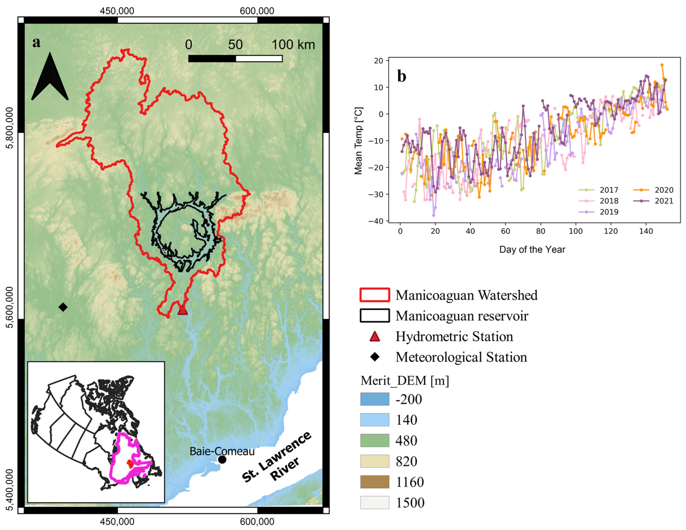
The study area is situated in the eastern part of Quebec province, Canada (Figure 1). The Manicouagan reservoir is part of the Manic-5 watershed, which is managed by Hydro-Quebec [27]. The Manicouagan River system, which originates in the Manicouagan reservoir, has a total installed capacity of approximately 5600 MW [27]. This river flows into the Saint Lawrence River near Baie-Comeau (Figure 1a), located ~190 km downstream of the Daniel-Johnson dam. The ring-like shape of the Manicouagan reservoir was generated by an asteroid that impacted the Earth 214 million years ago [28]. This reservoir has a surface area of 1788 km2 and a total volume of 138 km3 [27]. The watershed area is 29,000 km2 and has a rolling to moderately hilly topography, with a maximum elevation of 952 m above sea level.
For the 5-year winter periods of study, the mean temperature is −16 °C. An important amount of precipitation characterizes this mostly forested area (950 mm). The maximum floods usually occur during the spring season when snow and ice melt play an important role. During the winter period, ice thickness can reach significant values of more than 1 m [29]. The mean annual local flow is 528.89 m3/s [30].
3. Materials and Methods
An automated routine was implemented in Google Earth Engine (GEE) to investigate the spatiotemporal evolution of ice characteristics of the Manicouagan reservoir from optical and radar imagery for the period January to April from 2017 to 2021. Specifically, the surface temperatures from the Terra Land Surface Temperature (LST) and Emissivity 8-Day product (MOD11A2.006) from MODIS were used, as well as LSTs estimated from Landsat OLI 08. The methodology from Ermida et al. [31], freely available at https://github.com/sofiaermida/Landsat_SMW_LST (accessed on 1 June 2022), was implemented to compute LST time series from Landsat imagery. Landsat images were first atmospherically corrected and masked to reduce cloud contamination. Then, the LST maps were estimated using the Statistical Mono-Window algorithm from Climate Monitoring Satellite Application Facility (CM-SAF), which uses an empirical relationship between top-of-atmosphere (TOA) brightness temperatures in a single TIR channel and LST [31]. In both MODIS-based and Landsat-derived LSTs, quality information bands were used for cloud masking. Once the LST map series were produced, average daily LST values over the Manicouagan reservoir were computed for the target winter periods. In order to perform a general yearly inspection of the spatial distribution of surface temperature over the reservoir, mean MODIS and Landsat LST maps for each winter season were also produced and globally compared.
Equally, Sentinel-1 SAR Ground Range Detected (GRD) images were extracted and processed in Google Earth Engine. These products were acquired from January to April between 2017 and 2021. Two polarization configurations (VV and VH) were available for the data used. The VV polarization of the Sentinel-1 C-band was reported to perform better for lake ice applications than the VH polarization (e.g., [7]) and it was therefore selected in this study. The images were filtered to reduce the speckle noise using a Refined Lee filter with a moving window of 3 m by 3m (https://code.earthengine.google.com/5d1ed0a0f0417f098fdfd2fa137c3d0c*/ accessed on 1 June 2022) and masked to obtain the mean backscattering values over the reservoir. These products were used to evaluate the evolution of the C-band response to ice and the progress and state of ice coverage, which can be assessed from the development of linear features.
The ERA5-land dataset (0.1°, hourly) provides different types of land parameters at an enhanced resolution compared to its predecessor [32]. Because of its relatively fine spatiotemporal resolutions, ERA5-land can be very useful for different applications. Ice depth (ice thickness) and lake ice temperature variations over the Manicouagan reservoir were also investigated from these datasets. ERA5-land products were requested from the Copernicus Climate Change Service (https://cds.climate.copernicus.eu/ accessed on 1 September 2022). Estimates were then resampled at a daily time step for comparison with the satellite observations.
For part of the winter of 2018, the D-InSAR technique was used to potentially infer changes in ice thickness. The D-InSAR technique consists of a complex multiplication of two SAR images (interferogram) from which changes in the Earth’s surface can be derived. Sentinel-1 TOPSAR data in the Single Look Complex (SLC) Interferometric Wide (IW) mode were processed using the European Space Agency (ESA) SentiNel Application Platform (SNAP). To verify if the inferred changes were explained by the ice thickness variations or by other factors (e.g., water level fluctuations), the maps of radar backscatter were inspected along with in situ and altimetry-based water levels.
Altimetric data from Sentinel-3 and Jason-3 were requested from the Centre de Topographie des Océans et de l’Hydrosphère (CTOH) at LEGOS (Laboratoire d’études en Géophysique et océanographie spatiales). The altimetric data were post-processed using the Altis software [33]. To interpret and evaluate the quality of the surface height from these altimeters, they were compared to the available records of water levels from a hydrometric station (see Figure 1a). The evolution of radar backscattering values from the Ku-band of Sentinel-3 was also evaluated.
The Surface Water and Ocean Topography Mission (SWOT), launched in December 2022 and which first data are expected to be publicly available in late 2023, will provide critical information on inland waters; however, SWOT signal interaction with hydrometeorological variables such as ice or snow is not yet clearly established. As an experiment, SWOT products (pixel cloud) during winter were mimicked using the large-scale (LS) SWOT hydrology toolbox (SWOT-LS) developed by the Centre national d’études spatiales (CNES) (https://github.com/CNES/swot-hydrology-toolbox accessed on 1 September 2022). This synthetic analysis is produced by hypothesizing about the SWOT signal behavior in the presence of ice. The SWOT-LS simulator requires as input a contour mask and surface height information. For this experiment, altimetric-inferred water levels and contours from Sentinel-1 data were used as inputs. Science orbit 214 was selected because it covers most of the reservoir surface. Examples of mimicked SWOT products are presented and briefly discussed. We highlight that the cal/val orbit passes over the reservoir.
4. Results
4.1. Ice Surface Temperatures from Optical Imagery
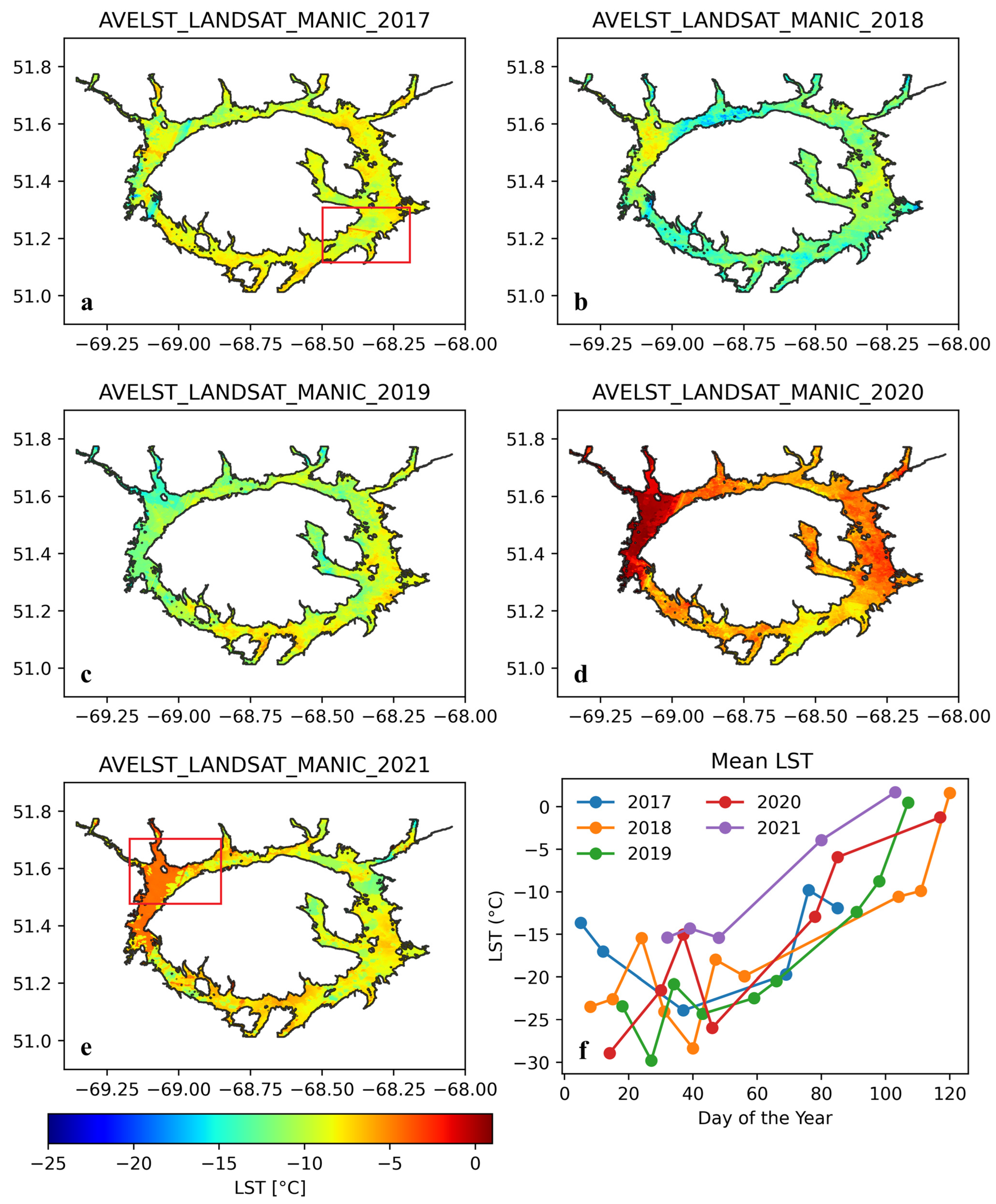
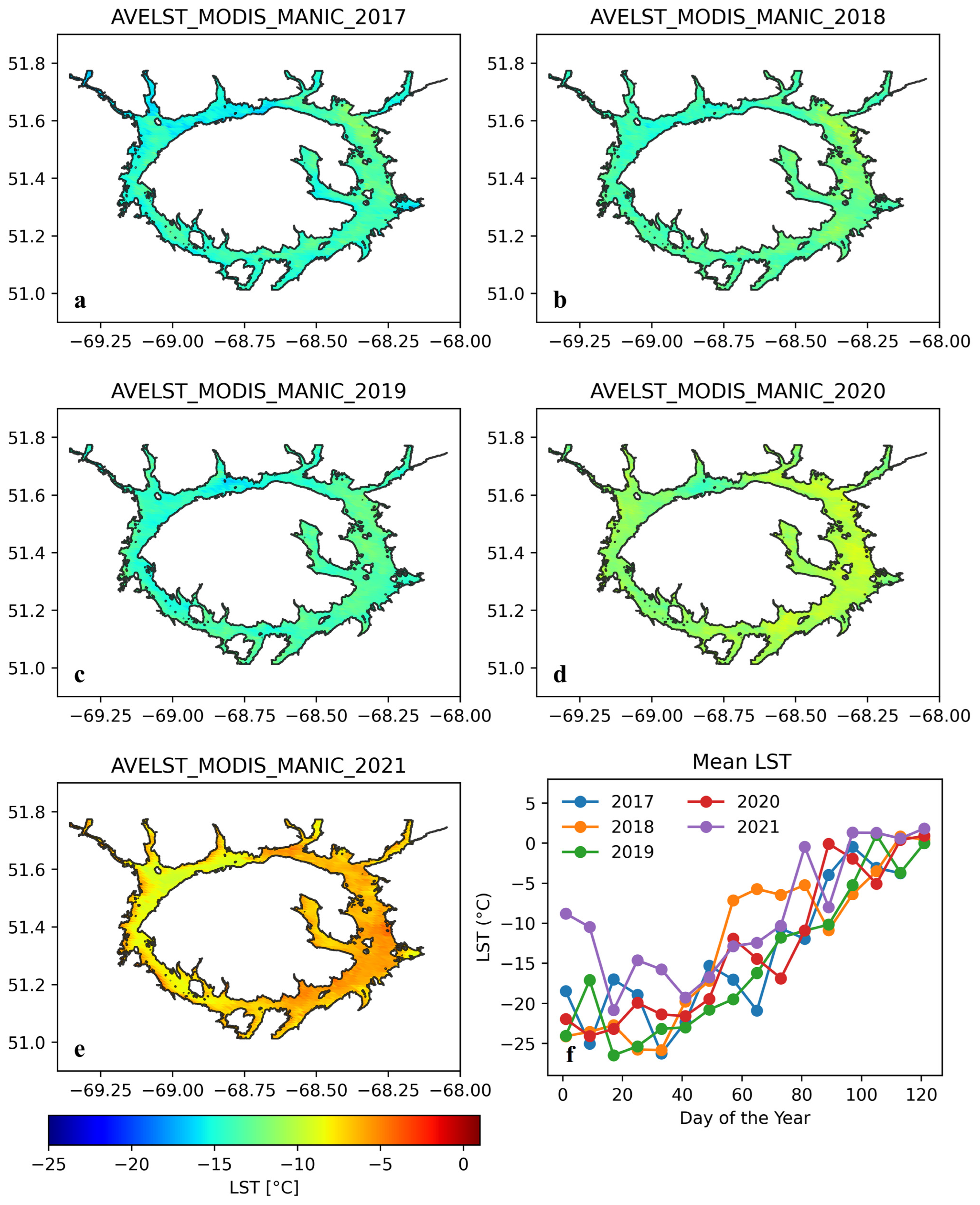
Land surface temperature (LST) over the Manicouagan reservoir from MODIS and Landsat imagery are visualized in Figure 2 and Figure 3, respectively. Specifically, Figure 2a–d and Figure 3a–d show maps of mean Landsat and MODIS LST, respectively, for the different winters under study. Mean daily LST time series from MODIS and Landsat are depicted in Figure 2f and Figure 3f, respectively. Spatially, the LSTs from both sensors vary over the reservoir for each winter. The concentration of high/low-temperature patches is observed, with their location changing from one winter to another. Landsat LSTs vary between −28 °C in January and near or slightly above 0 °C at the end of April. In the case of MODIS (Figure 3), a smoother spatial distribution of LST is observed for each winter, and LSTs vary on average from −25 °C to 0 °C from January to April.
4.2. Ice Backscatter and Cover from C-Band Imagery
The spatiotemporal evolution of average backscattering values σ0 through the different winter periods under study is presented in Figure 4. The spatial distribution varies from winter to winter. Important fracture development over the entire reservoir for each winter is observed (Figure 4a–e), suggesting that the reservoir is completely covered by ice. Overall, these linear features are associated with higher backscattering values. Some fractures occur at similar positions for specific winters (e.g., Figure 4b,d). A smoother spatial distribution of backscattering values over the reservoir is observed in winter 2021 compared to the other winters. Temporally, the radar backscatter signal, in general, increases as the winter advances from January until the end of March when a decay is observed (Figure 4f). The minimum values of radar backscatter are lower than −20 dB in January and, overall, larger than −16 dB in March. Values decrease by an average of 6 dB from the end of March to the end of April.
4.3. Ice Thickness Variation from ERA5-Land and D-InSAR
Figure 5 shows the evolution of the daily reservoir ice thickness from ERA5-land for the different winters of study. The mean daily ice thickness over the reservoir is observed to increase from January until, approximately, the end of March for all winters. Overall, a notable decay is observed from April. The maximum ice thickness estimated from ERA5-land varies between 1.1 to 1.4 m. The lowest ice thicknesses are observed in winter 2021 whereas the largest ice thicknesses in 2019. Figure 5b–d depict examples of maps that represent the spatial distribution of lake ice thickness as the winter advances. As observed, ice thickness varies over the reservoir. Overall, the larger ice thickness is observed at the northern part of the lake, while towards the southern and southeastern parts of the reservoir, ice thickness is smaller.
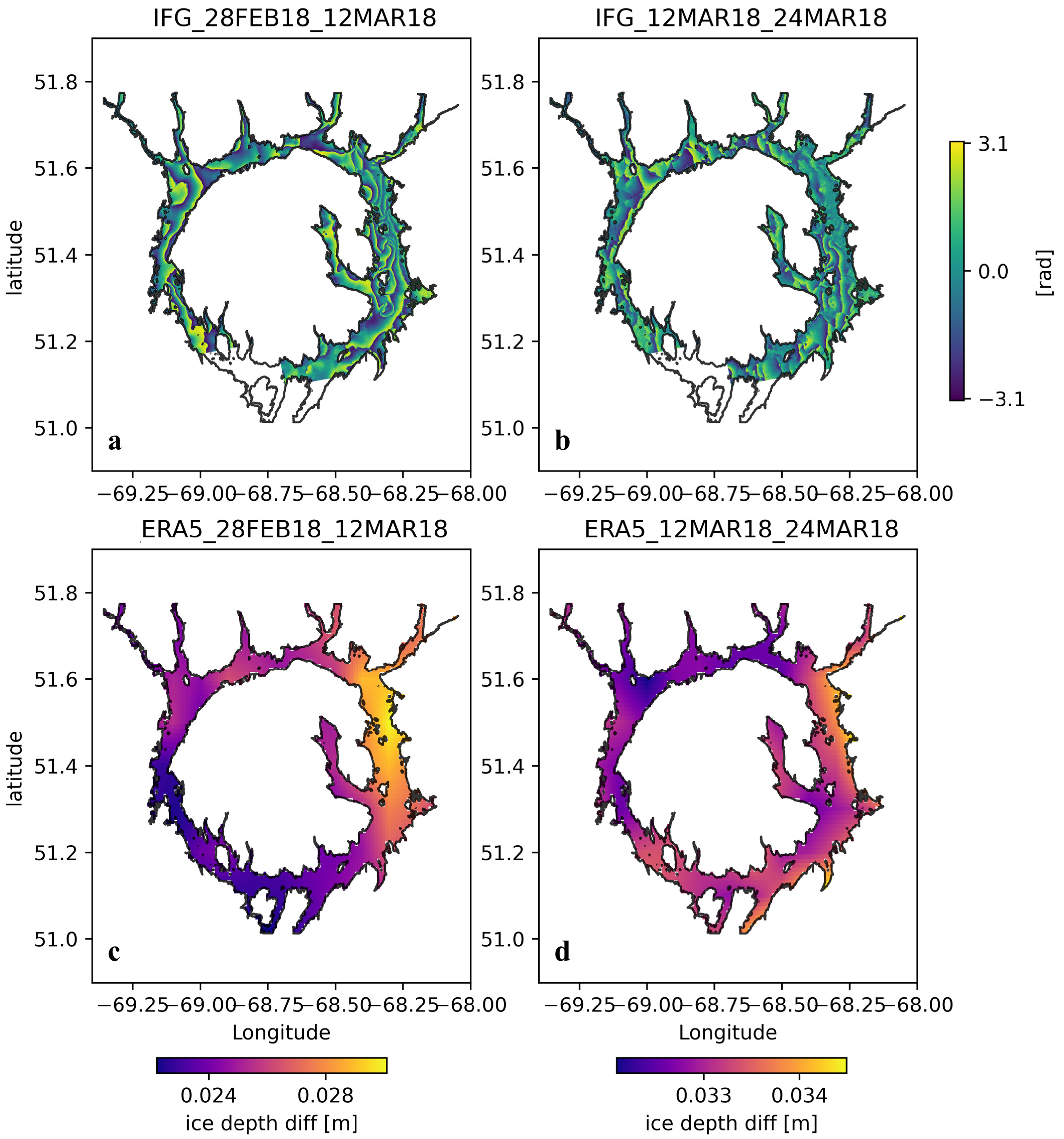
D-InSAR was explored to investigate surface changes during the winter over the Manicouagan reservoir. Interferograms were generated for the later stage of winter 2018, when coherence was maintained. Figure 6 shows the maps of surface changes between February and March estimated from D-InSAR. One fringe (color cycle) corresponds to a 2.8 cm range change along the satellite look direction. Considering an average incident angle of 36.5°, the vertical component of these changes is ~3.5 cm, which could be potentially related to ice thickness changes. Important changes of more than 10 cm are observed in some sectors of the lake (Figure 6a,b). Figure 6 also depicts the difference in ice thickness from the ERA5-land data estimated for the same dates of the SAR images used in the interferogram computation. Differences in ERA5-land ice thickness for the 12-day periods of analysis vary spatially and temporally, being larger (>3.5 cm) in March (Figure 6d). Unfortunately, coherence for winter 2019 to 2021 was not sufficiently maintained to generate good quality interferograms for those years and therefore they were not included in this study. The possible causes of decorrelation are analyzed in Section 5.
4.4. Water Levels and Reservoir Ice Evaluation from Altimetry Data
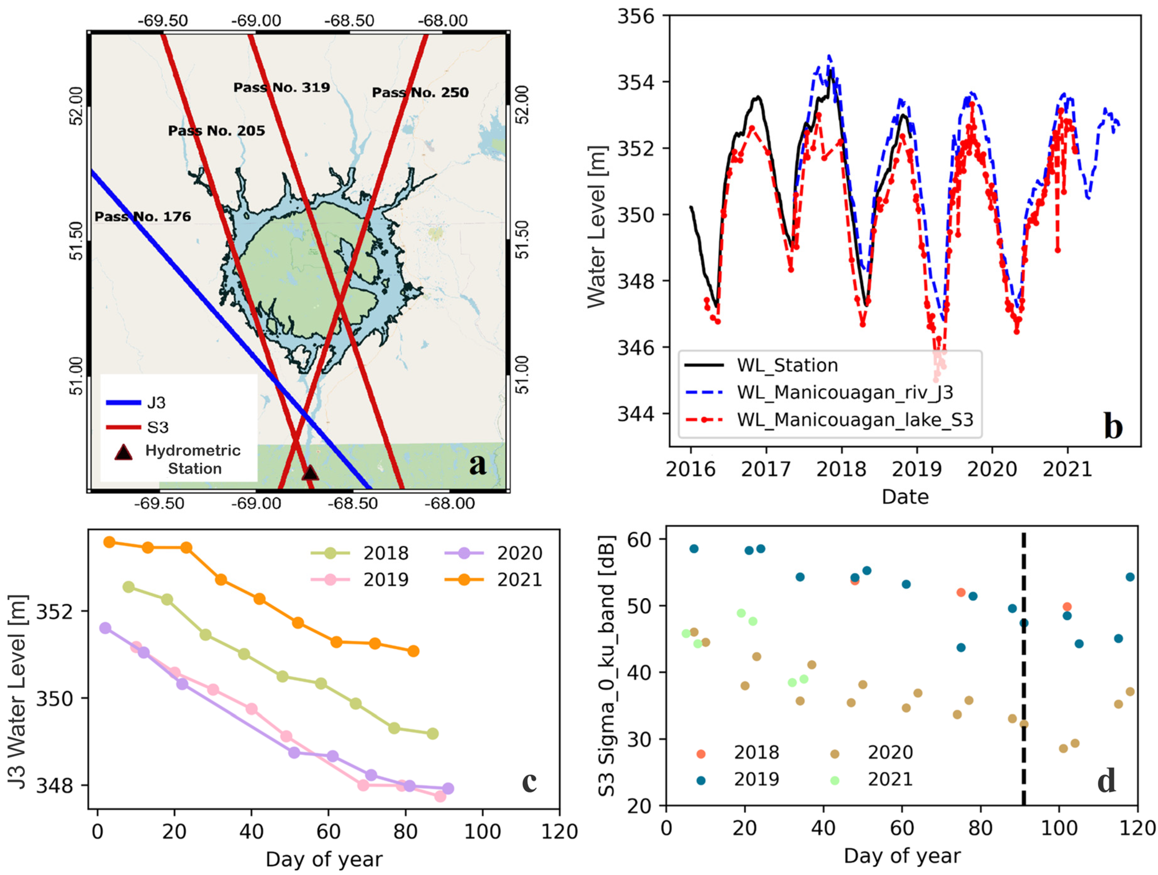
Analysis of altimetric data for the evaluation of water levels and reservoir ice is also included in this study (Figure 7). The time series of surface elevations between 2017 and 2021 extracted from altimeters Jason-3 and Sentinel-3 are depicted in Figure 7b. These series are compared to those from the hydrometric station to evaluate if the pattern observed corresponds to water level variations in the reservoir. Jason-3 observations are nearer to the hydrometric station located in the southern part of the reservoir, whereas Sentinel-3 passes over the ring-shaped area (Figure 7a). A similar pattern is observed between the altimeters and the hydrometric station time series, although Sentinel-3 surface elevations are lower. The Jason-3 water level series only for the winter period are depicted in Figure 7d. Jason-3 water levels notably vary from winter to winter, being the largest mean water level differences (>1 m) between winters 2019–2020 and winter 2021. The evolution of the radar backscattering of the Ku-band of Sentinel-3 is also presented (Figure 7d). Overall, values of the backscattering signal seem to steadily decrease as the winter advances.
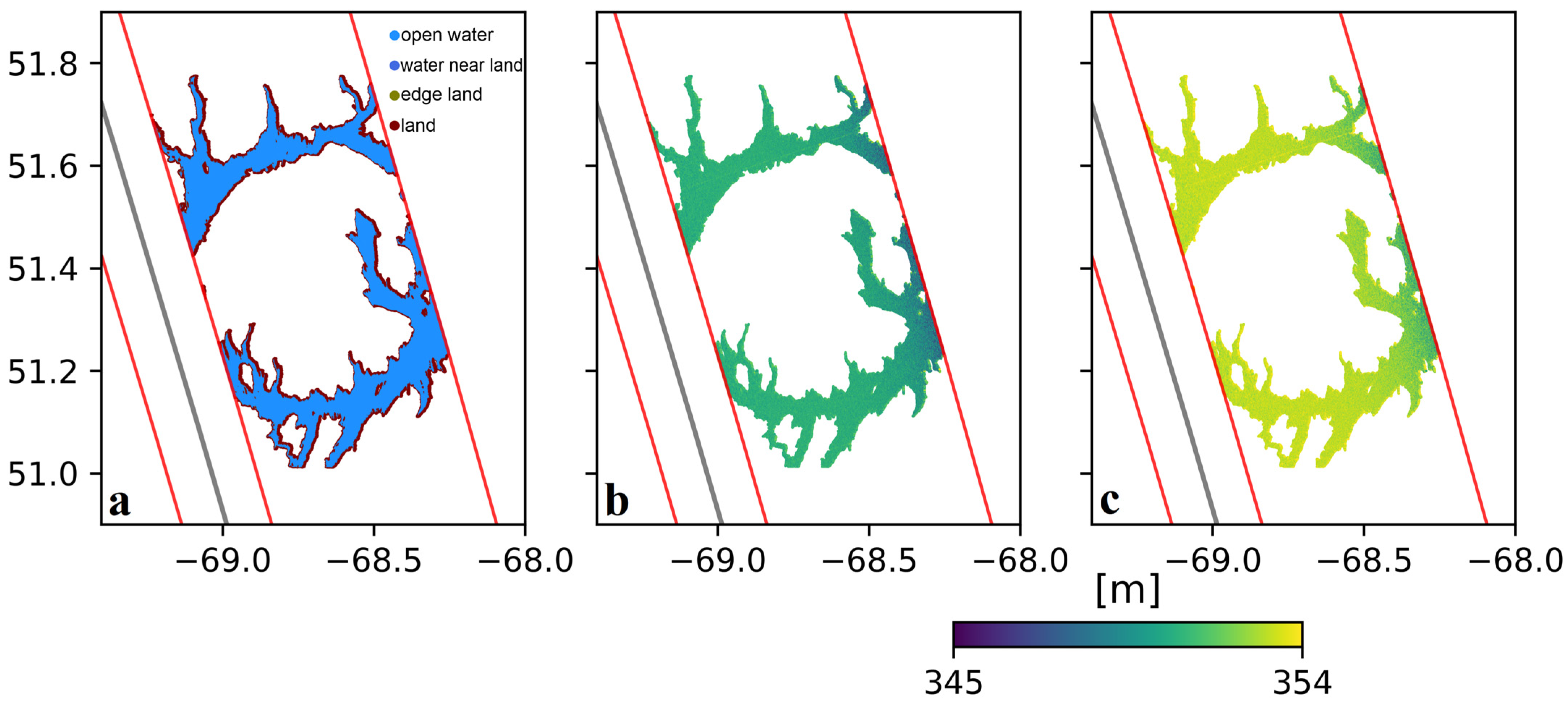
Figure 8 shows examples of SWOT pixel cloud products generated by the SWOT-LS simulator from the CNES. Figure 8a depicts the classification that considers four different classes for the current simulation (open water, water near land, edge land and land). Most pixels (91%) belong to the water class (4), whereas the land class is the least populated. The spatial distribution of surface elevations for the maximum winter water levels of 2019 and 2021 is represented in Figure 8b and 8c, respectively. Water levels for classes 3 and 4 are centered around 351.17 m for the winter of 2019 and around 353.58 m for the winter of 2021.
5. Discussion
5.1. Ice Surface Temperatures from Optical Imagery
Spatiotemporal evolution of land surface temperatures from Landsat and MODIS was studied over the Manicouagan reservoir for the winter seasons from 2017 to 2021. Although time series from both MODIS and Landsat indicate increasing LSTs as the winter advances, the latter present important gaps due to, for example, cloud filtering. Therefore, the important LST jumps observed in the MODIS LST time series are not captured by the Landsat series. Important fluctuations in the MODIS time series are principally observed at the beginning and the end of the winter, which could be linked to changes in the ice coverage state (initial formation and decay, respectively). From the hydrometric station, important air temperature variations are also noted at several moments of each winter period (Figure 1). Note that this station is located at more than 100 km from the reservoir; thus, variations might not precisely reflect the conditions over the reservoir. According to the records of this station, the hottest winter was that of 2021 (mean temperature of −13 °C), followed by the winter of 2020 with a mean air temperature of −15 °C. These observations agree with those derived from the mean LST satellite-based time series (Figure 2f and Figure 3f) and from the ERA5-land data. In general, temperatures for the yearly winter periods of study from both sensors are similar. For the five winter periods of study, the average variation of temperature in the case of MODIS is 25 °C, whereas, in the case of Landsat, it is around 28°C.
Spatially, LST maps from MODIS are smoother compared to the LST maps from Landsat principally due to the difference in resolution. Note that the mean LST maps can be influenced by some unusually warm periods of time. The maps of the mean Landsat LSTs are estimated from a lower density of daily LST images, and therefore the effect of these warm periods is more evident in this case (e.g., Figure 2d). In both cases (Figure 2 and Figure 3), the distribution of mean LST values over the reservoir varies from year to year, although no clear pattern of LST was identified in these maps. In some areas, Landsat LST maps show notable local gradients (Figure 3); remaining clouds, shadow contamination and the averaging process can cause these important LST contrasts. The mean LSTs for both sensors remain below zero over the entire reservoir for almost every winter, suggesting that the reservoir may be completely covered by ice from January to March for those years.
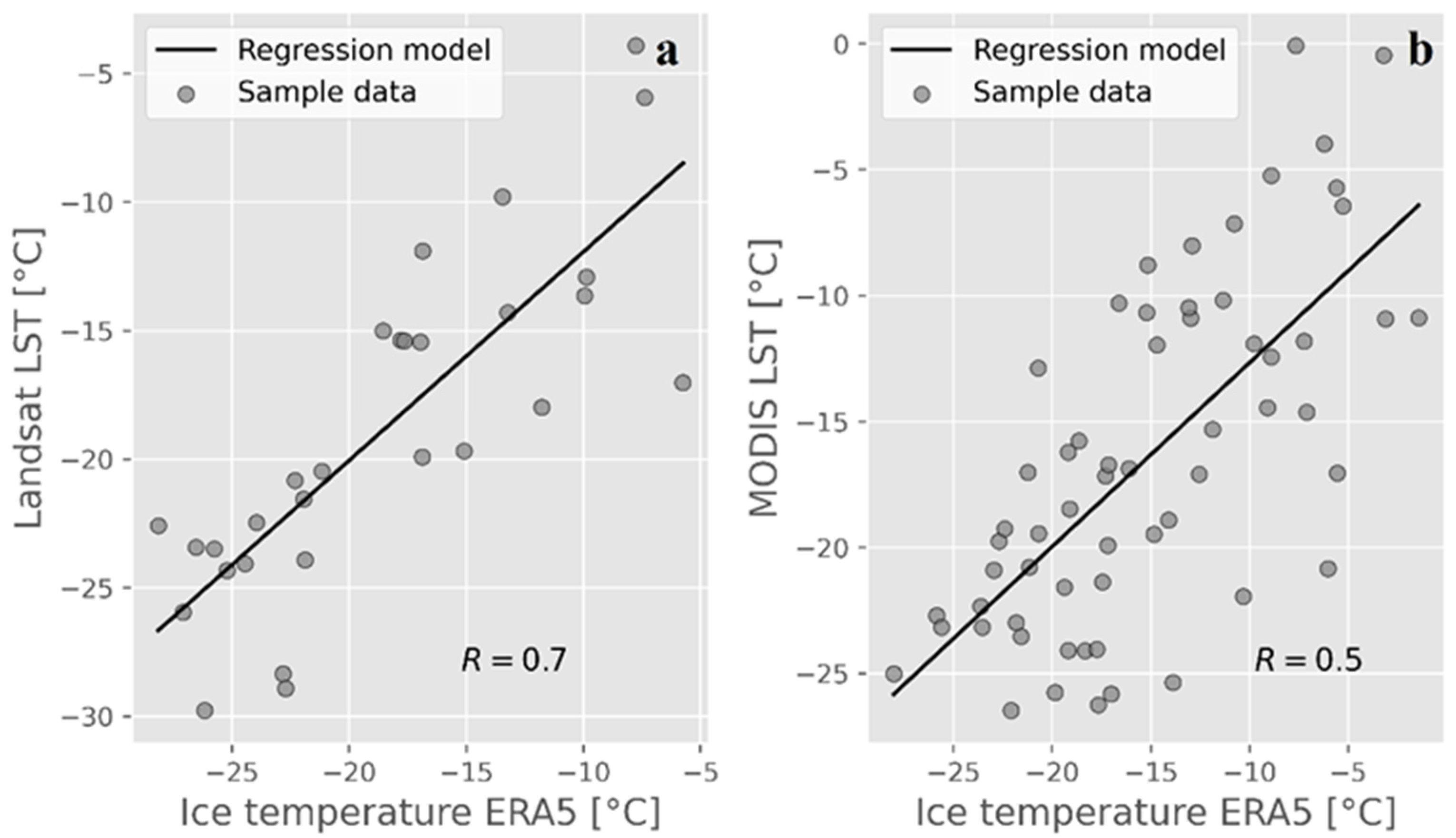
To further validate the satellite-based LST from MODIS and Landsat, they were compared to the lake ice surface temperature from ERA5-land reanalysis; the Pearson correlation coefficient, the Root Mean Square (RMSE) and the absolute differences were included in the comparative evaluation. In Figure 9a, ice temperatures from ERA5-land range from −28 °C to −1 °C for the dates of the Landsat acquisitions, whereas they rang from −28 °C to 1 °C for the dates of the MODIS imagery. The Pearson correlation coefficient (R) of 0.7 is observed between the surface temperature from ERA5-land and Landsat, and 0.5 between the MODIS LST and the ERA5-land ice temperature. These analyses indicate an overall good linear association between the reservoir’s uppermost surface temperature of ice and the surface temperature inferred from these optical sensors. Nevertheless, a better correlation is achieved between the LST from Landsat and the ice temperature from ERA5-land. A similar validation assessment was performed between the air temperatures from the meteorological station and the satellite-based LSTs, indicating a correlation of 0.5 and 0.7 when comparing them against LSTs from MODIS and Landsat, respectively.
Regarding the RMSE, after outlier removal, a value of 3.7 °C was estimated in the case of the Landsat–ERA5-land comparison and 5.2 °C in the case of MODIS–ERA5-land. The absolute differences of surface temperatures from Landsat and ERA5-land for the winter periods of study vary between 6 °C and 0 °C, and, in the case of MODIS–ERA5-land, between 9 °C and 0 °C. The estimated absolute differences and correlations between surface temperature from MODIS and ERA5-land are within the range found by other studies at a global scale using monthly temperature values (e.g., [34]). Similarly, the RMSEs correspond to values estimated in existing studies(e.g., [23]). We highlight that correlation and RMSE in those studies used skin temperature in the comparison and over a larger period of time, whereas this study focused on reservoir ice temperature during the winter season over a 5-year period.
Although cloud masking was applied to the satellite imagery, the remaining cloudy pixels might influence the quality of the LST measures and, therefore, the interpretation and the quality of the regression analysis. Moreover, the retrieved LST of some pixels over the reservoir could correspond to snow, which could also impact the comparative analysis against the ERA5-land data. Some recent methods have been proposed to reduce cloud presence in MODIS snow cover products [35]. These methods could be explored to discriminate between ice and snow and their corresponding LST values.
5.2. Ice Backscatter and Cover from C-Band Imagery
The spatiotemporal analysis of Sentinel-1 backscattering coefficients over Manicouagan reservoir are also evaluated (Figure 4). As observed from the 5-year winter period of analysis, overall, the radar backscattering coefficients increase as the winter advances from January to April, when a notable decay is observed (beginning of break-up). Specifically, the radar backscattering coefficient over the entire reservoir varies on average between −19 dB at the beginning of the winter and −15 dB at the end of March. At this moment, temperatures start to notably increase, being above or near 0 °C. Previous studies over Canadian lakes have reported similar trends of the break-up dates for longer periods of analysis (e.g., [36]). Possibly, the early break-up date observed may be caused by a combined effect of changes in temperature, snow cover and wind conditions (e.g., [37]).
In general, the temporal variation of mean backscattering values for the ice-on season agrees with those reported by other studies (e.g., [4]). Very low backscattering values (<−20 dB) have been associated in previous studies with grounded ice (e.g., [4,7]). Grounded ice might occur at the shores of the lake and of the islands within the reservoir; however, low values are also observed at the center of the reservoir (Figure 4). Considering the water depth at these locations, the low radar backscattering in this case might be related to the ice structure (low presence of air inclusions) and to the smooth ice/water interface which might remain stable (e.g., [38]). Regions of higher values of radar backscattering are possibly related to the ice cover formation process, where a thin layer of rough ice was formed because of wind effects, resulting in a rough ice/water interface that remained throughout winter. Deformation in the form of ice fractures is associated with relatively higher values of backscattering, possibly due to a strong surface roughness. These ice deformation elements can be useful to identify the progress of the ice coverage. Note that some of the features remain throughout the winter as suggested by the mean backscattering maps (Figure 4) and evaluation of individual backscattering maps. Usually, from April on, important snow and ice melting due to higher temperatures occur, and therefore, the mean backscatter maps are estimated from January to March. The decrease of radar backscattering coefficients at the late stages of the winter (Figure 4c) could be explained by the specular backscattering due to ice-snow melting, water overflooding the ice or a combined effect of both. It must be highlighted that a notable increase in water levels associated with the break-up occurs in the middle of April.
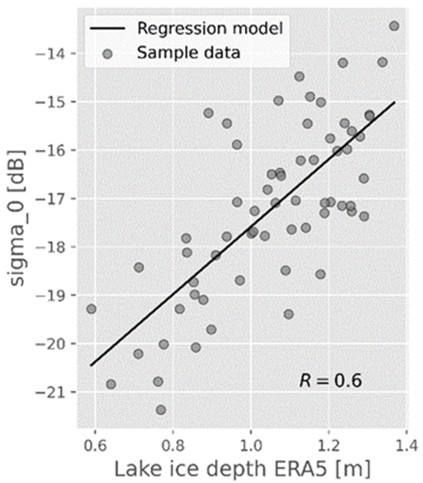
The radar backscattering values were also compared to the ice thickness values from ERA 5-land to evaluate a possible relationship between these two variables (Figure 10). A relatively good correlation(R) of 0.6 was found for the 5-year winter periods of analysis. These results agree with those from existing studies, which suggest that ice growth is linked to an increase in radar backscattering values independent of the format of air inclusions (e.g., [12,19]). The value of the correlation obtained indicates that ice growth could be approximately modeled linearly as a function of the radar backscattering coefficient; nevertheless, a longer time series of datasets needs to be evaluated to conclude the relationship of these variables and to propose a model that could be used for forecasting purposes and the calibration of physical lake ice models.
5.3. Ice Thickness Variations from ERA5-Land and D-InSAR
The variations of ice thickness over the reservoir were studied from the ERA5-land datasets. For the five years of study, the ice thickness of the reservoir grew progressively following an approximately linear trend. This ERA5-land parameter represents the behavior of a single ice layer, but the ice structure is typically composed of several sublayers. This simplification does not consider the possible interactions between layers and the different elements (e.g., lenses, air bubbles, impurities) that could actually impact the growth and thickness values of the total ice layer. Nevertheless, assuming ice growth as a function of satellite-based surface temperature, which increases approximately linearly with time (Figure 2 and Figure 3), the ERA5-land ice thickness estimations could be considered an acceptable approximation. Note that the largest ice thickness (1.4 m; Figure 5a) occurs in 2019 when the coldest temperatures are also identified from the satellite LST time series (Figure 2 and Figure 3). The smallest ice thickness corresponds to winter 2021, which is the hottest winter of the 5-year period of study. From the ERA5-land datasets (Figure 5b–d), smaller ice thickness forms towards the southern parts of the reservoir, possibly due to local variations of climate conditions. The reservoir is very large, and north–south air temperature gradients exist.
As part of this research, the potential of D-InSAR to extract additional information on ice dynamics was also evaluated and analyzed along with the ERA5-land data. Critical coherence (a measure of interferogram reliability) loss occurred in most winter periods, affecting the quality of the phase changes. However, for winter 2018, SAR returns were stable enough to preserve coherence over temporal baselines of 12 days. Particularly, two interferograms between February and March were studied and compared to maps of ERA5-land ice thickness difference estimated for the same dates. From the analysis of the Sentinel-1 backscattering and the LST maps, the reservoir is expected to be completely covered by ice for the period covered by the interferograms in Figure 6. This might suggest that the vertical component of the D-InSAR-based changes is predominant and that they could be explained in part by ice thickness changes but also by water level variations due to hydraulic operations (Figure 7) or a combined effect of these elements. Moreover, the detected D-InSAR variations may reflect changes in the part of the ice thickness above the water line. Notwithstanding, lateral displacement is not completely discarded. Important phase gradients are observed, particularly in the east arm of the lake and, more notably, in the interferogram pair 28 February–12 March (Figure 6a), where vertical changes >10 cm are observed. For the same pair, changes of up to ~4 cm are identified at the western arm of the reservoir. Note that these patterns seem to approximately remain in the interferogram pair between 12 and 24 March 2018, although signal degradation seems to occur in some portions of the lake. This deterioration of the signal can possibly be caused by ice–snow melting or an overflooded ice surface. The maximum ice thickness found to be reported for the reservoir varies between 1 m and 1.5 m [31]. Considering these reported values and a linear ice growth from January to March, the maximum ice thickness changes for a 12-day period are estimated to be (12–15) cm. These values approximately correspond to the maximum range of vertical changes inferred from D-InSAR for the winter of 2018. Because altimetric data was not available for the dates of the interferogram pairs, information from the hydrometric station was used to evaluate if a component of the vertical movements is related to fluctuations in the water levels. The difference in water levels for the two 12 day-periods of the interferogram remains stable (~60 cm). This value is much larger than the measured phase changes. However, the station provides punctual data and is located at an important distance (>40 km) from the reservoir. Despite its location, the limnometric station records provide a reasonable estimation of water level changes in the reservoir.
Maps of ERA5-land ice thickness difference were estimated and compared to the interferograms to verify if similar patterns are found (Figure 6c,d). Ice thickness differences vary between 2.2 cm and 3.5 cm for the period between 28 February and 24 March, 2018. We remark that the sector of large ice thickness differences in the eastern part of the reservoir roughly coincides with the location of important D-InSAR vertical changes. This inspection encourages the hypothesis that phase changes could be associated with ice thickness changes. Nevertheless, a denser number of coherent interferograms and in situ data might be necessary to validate this interpretation. Moreover, in situ measurements might be required to validate the results of the simulated ice thickness by the ERA5-land model.
5.4. Water Levels and Reservoir Ice Evaluation from Altimetry Data
Altimetry data from Sentinel-3 and Jason-3 data was explored to support the analysis of ice and winter water level conditions over the Manicouagan reservoir. The estimated time series from both sensors were examined and compared to the water levels from the available hydrometric station during the ice-on and ice-off periods. The objective of this comparison is to support the interpretation of the patterns observed in the altimetric data. In general, Jason-3 elevations are higher than the water level at the station, whereas Sentinel-3 heights are lower, particularly in the ice-off period. The RMSE between the water levels from the station and the altimetric surface heights are 0.6 m (0.5 m only winter period) and 0.8 m (1.2 m only winter) for Jason-3 and Sentinel-3, respectively. The Pearson correlation coefficients are 0.99 and 0.97, respectively, for the Jason-3 versus the station data and for the Sentinel-3 versus the station data. A consistent pattern of the in situ and the altimetric-based time series is observed, suggesting that the radar pulses from these altimeters might penetrate the ice. Thus, the altimetric inferred surface heights in winter can be principally associated with water levels. We highlight that hydropower generation plays an important role in water level regulation. Previous studies have also reported the capabilities of these sensors to measure water levels under ice and/or snow (e.g., [39]). Differences observed in water levels between the satellite-based and the gauge observations are partially caused by the different locations of the altimeters’ ground tracks and the station. Jason-3 time series were generated from a track closer to the gauge station, whereas, in the case of Sentinel-3, all ground tracks within the reservoir perimeter were used; this could partially explain why the variations with respect to the in-situ time series are smaller compared to those from Sentinel-3. Deviations from the in-situ measurements can also be caused by the presence of ice in the winter period, which can affect the quality of the retrieved signal from the water/ice interface. Shu et al. [39] suggest that these differences increase with the ice thickening throughout the winter. Absolute differences between the gauge and Jason-3 water levels for the winter period vary between 0.30 cm and 0.80 cm, being the mean difference of 0.5 cm. Differences are larger than 1 m when comparing gauge water levels to those from Sentinel-3 data for the winter period; important outliers were detected and filtered out the Sentinel-3 data. In general, the series of Jason-3 data used have better temporal coverage than the series of Sentinel-3 data for the 2018–2021 winter periods (Figure 7b). The Jason-3 time series indicate an overall progressive decrease in water levels as the winter advances (whereas ice depth increases; Figure 5a), although some periods of stable water levels can also be observed (Figure 7c).
Another parameter analyzed in this study was the Sentinel-3 Ku-band radar backscattering signal (Figure 7d). The time series of backscattering coefficients recovered from all the tracks indicate that radar backscattering decreases as the winter advances. This effect is particularly visible for the years 2019 and 2020, when the temporal coverage is better. Specifically, the radar backscattering of Sentinel-3 Ku-band decreases until the end of March when it starts to increase again. Note that the evolution of the Ku-band radar backscattering is the opposite of the C-band from Sentinel-1. The differences observed are principally due to the band frequency and the geometry of observation, which influence the interaction of the radar signal with the physical medium (ice, snow/ice, water ice) and, therefore, the strength of the radar backscatter returns. Because snow grain and ice bubble sizes are closer to the Ku wavelength than to C-band, more scattering is expected from the Ku band as snow/ice thickness increases. Whereas snow/ice is more transparent to the C-band signal, attenuation of the signal, although small, comes into play. Mahmud et al. [40] show a case where a similar effect is observed between modeled C- and Ku-band backscatter signatures. The range of variation of the radar backscattering notably differs between these two sensors. The mean Sentinel-3 backscattering coefficient varies between 28 dB and 69 dB between January and March compared to the (−21 dB to −13 dB) variation of Sentinel-1.
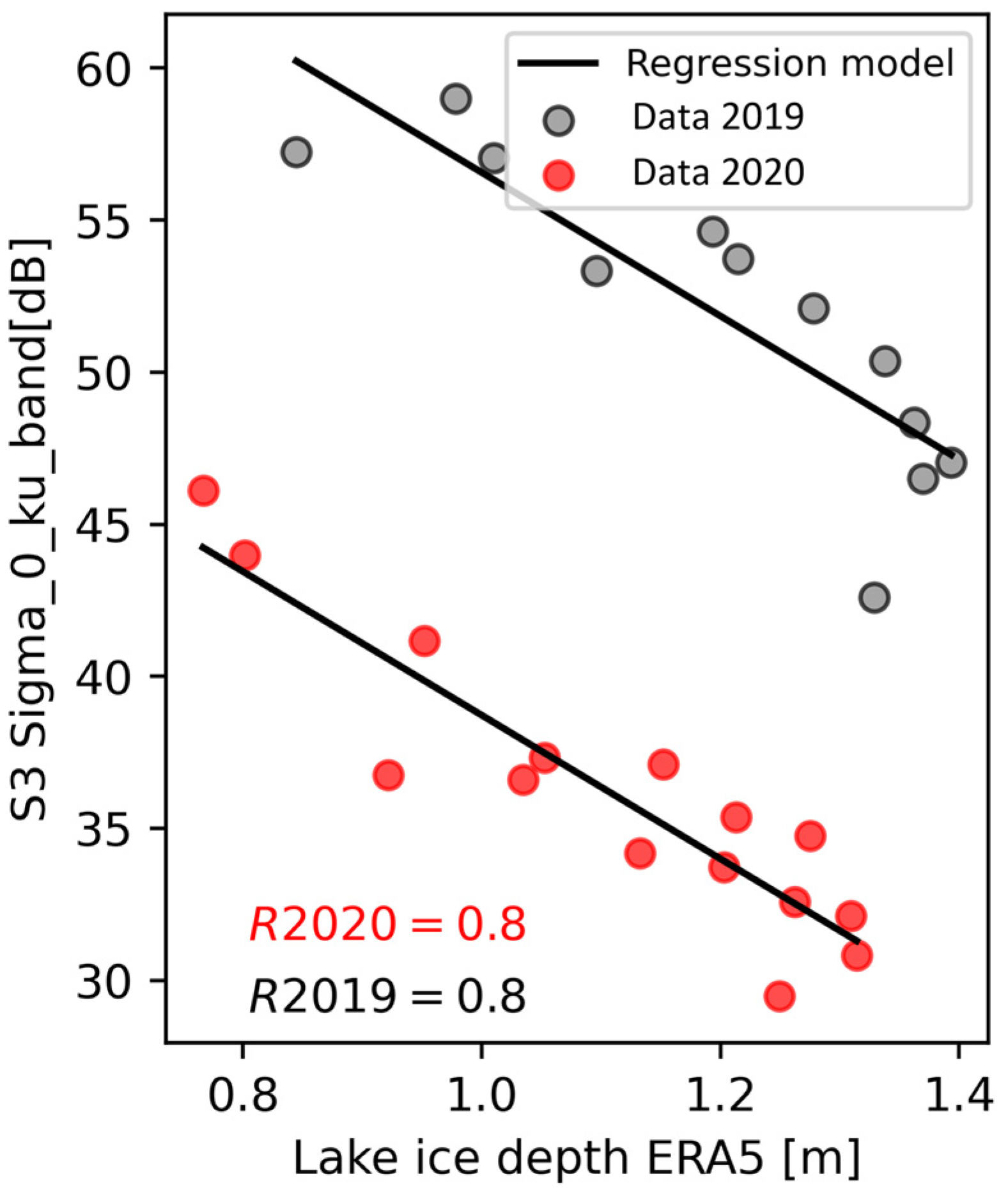
The Sentinel-3 radar backscattering values were compared to the ice thickness values from ERA 5-land to evaluate a possible relationship between these two variables (Figure 11). Because of the important variations in the magnitude of the Sentinel-3 radar signal from year to year, we evaluate this relationship separately for the years 2019 and 2020, for which we have better data sampling (Figure 7d). A correlation coefficient R of 0.8 and was found, suggesting that a model of ice thickness growth as a function of the Ku-band backscattering signal could be explored. Despite the almost 15 dB difference between the two curves in Figure 11, with higher values in 2019 compared to 2020, the slopes are nearly identical. Identical slopes imply similar scattering behavior; the 15 dB difference perhaps can be due to surface roughness differences, being that the ice/water interface was rougher in 2019.
This section also briefly discusses proxy SWOT products, which were generated with inputs from optical and altimetric data acquired during the winter period. Specifically, examples of pixel classification and surface height distribution were generated and examined (Figure 8). The classification of pixels by the SWOT-LS simulator principally considered two main classes (land and water) with subclasses among them (land_near_water, water_near_land, open_water, dark_water, low_coh_water_near_land, open_low_coh_water). In this case, four of these subclasses were considered in the classification process, but the surface height evaluation was performed only on pixels that correspond to the interior and the water near land classes. The land and the edge land pixels observed in Figure 8a might, in fact, correspond to frozen sediments in the winter, whereas the other water classes might correspond to ice and/or water depending on the actual penetration capability of the SWOT signal. This capability will also be limited by the state of the upper snow and ice layer. Processes such as the melting of snow/ice could produce backscatter in all directions, therefore impacting the return signal (e.g., [41]). A more refined classification might be required considering actual values of SWOT backscatter under the presence of ice. Using the maximum surface elevations derived from altimetric data for the winters of 2019 and 2021, SWOT surface heights were simulated (Figure 8b,c). These maps represent a simplified distribution of surface heights. We highlight that only the mean average height was considered for the entire lake as an input, which might not be representative of the actual spatial variation. A slope is observed towards the east part of the reservoir; this effect could be produced by uncertainties linked to the proximity of pixels at these positions to the far range of the swath where errors are expected to increase [42]. By analyzing the distribution of heights, differences larger than 2 m were estimated between the west and the east part of the reservoir. However, the mean simulated values of height over the lake agree with the input height. A more realistic simulation could have been performed by using a grid of heights; however, this was out of the scope of this investigation. There are still several unknowns about the actual interaction of the SWOT signal with ice and snow that will be unveiled when the first SWOT data during the ice-on period will be available.
6. Conclusions
This study provides an assessment of the ice conditions of the Manicouagan hydroelectric reservoir for a 5-year period based on optical, radar and ERA5 reanalysis data. Optical data suggest important spatiotemporal variations of surface temperatures from year to year that are compatible with those from ERA5-land. Surface temperatures, overall, increase from January, being mostly above zero in April. The C-band scattering coefficient from Sentinel-1 increases as the winter advances until the end of March, when decay is observed. In the case of the Ku-band from Sentinel-3, the opposite occurs. Notable D-InSAR ice changes are noted approximately at the locations where maximum ERA5-land ice thickness differences are observed, suggesting that D-InSAR derived changes could be related to ice thickness changes, although a more in-depth analysis is required using a denser number of interferograms and in situ measurements.
Overall, winter water levels from altimetric data suggest a general decrease from January to March, presenting more fluctuations in the Sentinel-3 series than in the Jason-3 time series. The interpretation of the SWOT data mimicked using the SWOT-LS simulator suggests that a refined classification might be required to discriminate between water and ice during the ice-on season. Considering the behavior of the Ku-band signal from Sentinel-3 and Jason-3, which seems capable of measuring the water levels at the water/ice interface, a higher frequency sensor such as the SWOT KaRIn might perform well at retrieving information from this interface. Nevertheless, these assumptions will be tested once the actual SWOT winter data are processed and analyzed.
Author Contributions
Conceptualization, G.L.S.; methodology, G.L.S.; validation, G.L.S.; formal analysis, G.L.S. and R.L.; writing—original draft preparation, G.L.S.; review, supervision and editing, G.L.S. and R.L. All authors have read and agreed to the published version of the manuscript.
Funding
This research received no external funding.
Data Availability Statement
tThe data presented in this study are available upon request from the corresponding author.
Acknowledgments
The first author thanks the Fonds de recherche du Québec—Nature et technologies (FRQNT) for their support under the B3X program. We would like to thank our industrial partners: Hydro-Quebec, Brook Field and the city of Sherbrooke. The authors acknowledge the anonymous reviewers for their constructive comments toward an improved version of the manuscript.
Conflicts of Interest
The authors declare no conflict of interest.
References
- Magnuson, J.J.; Robertson, D.M.; Benson, B.J.; Wayne, R.H.; Livingstone, D.M.; Arai, T.; Assel, R.A.; Barry, R.G.; Card, V.; Kuusisto, E.; et al. Historical trends in lake and river ice cover in the northern hemisphere. Science 2000, 289, 1743–1746. [Google Scholar] [CrossRef]
- Gebre, S.; Alfredsen, K.; Lia, L.; Stickler, M.; Tesaker, E. Review of ice effects on hydropower systems. J. Cold Reg. Eng. 2013, 27, 196–222. [Google Scholar] [CrossRef]
- Huokuna, M. Ice jams in Pori. In Proceedings of the 14th Workshop on the Hydraulics of Ice Covered Rivers, Quebec, QC, Canada, 19–22 June 2007; CGU-HS Committee on River Ice Processes and the Environment. Available online: http://cripe.ca/docs/proceedings/19/Huokuna-et-al-2017.pdf (accessed on 1 January 2021).
- Tian, B.; Li, Z.; Engram, M.J.; Niu, F.; Tang, P.; Zou, P.; Xu, J. Characterizing C-band backscattering from thermokarst lake ice on the Qinghai–Tibet Plateau. ISPRS J. Photogramm. Remote Sens. 2015, 104, 63–76. [Google Scholar] [CrossRef]
- Beaton, A.; Whaley, R.; Corston, K.; Kenny, F. Identifying historic river ice breakup timing using MODIS and Google Earth Engine in support of operational flood monitoring in Northern Ontario. Remote Sens. Environ. 2019, 224, 352–364. [Google Scholar] [CrossRef]
- Zhang, S.; Pavelsky, T.M. Remote Sensing of Lake Ice Phenology across a Range of Lakes Sizes, ME, USA. Remote Sens. 2019, 11, 1718. [Google Scholar] [CrossRef]
- Siles, G.; Leconte, R.; Peters, D. Retrieval of Lake Ice Characteristics from SAR Imagery. Can. J. Remote Sens. 2022, 48, 379–399. [Google Scholar] [CrossRef]
- Leppäranta, M. Modelling the Formation and Decay of Lake Ice. In The Impact of Climate Change on European Lakes; George, G., Ed.; Aquatic Ecology Series; Springer: Dordrecht, The Netherlands, 2010; Volume 4. [Google Scholar] [CrossRef]
- Lofgren, B.M.; Zhu, Y. Surface energy fluxes on the Great Lakes based on satellite-observed surface temperatures 1992 to 1995. J. Great Lakes Res. 2000, 26, 305–314. [Google Scholar] [CrossRef]
- Latifovic, R.; Pouliot, D. Analysis of climate change impacts on lake ice phenology in Canada using the historical satellite data record. Remote Sens. Environ. 2007, 106, 492–507. [Google Scholar] [CrossRef]
- Kang, K.K.; Duguay, C.R.; Howell, S.E.L.; Derksen, C.P.; Kelly, R.E.J. Sensitivity of AMSR-E Brightness Temperatures to the Seasonal Evolution of Lake Ice Thickness. IEEE Geosci. Remote Sens Lett. 2010, 7, 751–755. [Google Scholar] [CrossRef]
- Gherboudj, I.; Bernier, M.; Leconte, R. A Backscatter Modeling for River Ice: Analysis and Numerical Results. IEEE Trans. Geosci. Remote Sens. 2010, 48, 1788–1798. [Google Scholar] [CrossRef]
- Pour, H.K.; Duguay, C.R.; Scott, A.; Kang, K.-K. Improvement of lake ice thickness retrieval from MODIS satellite data using a thermodynamic model. IEEE Trans. Geosci. Remote Sens. 2017, 55, 5956–5965. [Google Scholar] [CrossRef]
- Desrochers, N.M.; Peters, D.L.; Siles, G.; Cauvier Charest, E.; Trudel, M.; Leconte, R. A Remote Sensing View of the 2020 Extreme Lake-Expansion Flood Event into the Peace–Athabasca Delta Floodplain—Implications for the Future SWOT Mission. Remote Sens. 2023, 15, 1278. [Google Scholar] [CrossRef]
- Kouraev, A.V.; Semovski, S.; Shimaraev, M.; Mognard, N.; Legresy, B.; Rémy, F. Observations of Lake Baikal ice from satellite altimetry and radiometry. Remote Sens. Environ. 2007, 108, 240–253. [Google Scholar] [CrossRef]
- Beckers, J.F.; Casey, J.A.; Haas, C. Retrievals of lake ice thickness from great slave lake and great bear lake using CryoSat-2. IEEE Trans. Geosci. Remote Sens. 2017, 55, 3708–3720. [Google Scholar] [CrossRef]
- Mangilli, A.; Thibaut, P.; Duguay, C.R.; Murfitt, J. A New Approach for the Estimation of Lake Ice Thickness From Conventional Radar Altimetry. IEEE Trans. Geosci. Remote Sens. 2022, 60, 4305515. [Google Scholar] [CrossRef]
- Wakabayashi, H.; Motohashi, K.; Maezawa, N. Monitoring lake ice in Northern Alaska with backscattering and interferometric approaches using Sentinel-1 Sar Data. In Proceedings of the 2019 IEEE International Geoscience and Remote Sensing Symposium, Yokohama, Japan, 28 July–2 August 2019. [Google Scholar] [CrossRef]
- Murfitt, J.; Duguay, C.R. 50 years of lake ice research from active microwave remote sensing: Progress and prospects. Remote Sens. Environ. 2021, 264, 112616. [Google Scholar] [CrossRef]
- Brown, L.C.; Duguay, C.R. Modelling lake ice phenology with an examination of satellite-detected subgrid cell variability. Adv. Meteorol. 2011, 2011, 529064. [Google Scholar] [CrossRef]
- Rybushkina, G.; Troitskaya, Y.; Soustova, I. Ice cover determination of the Volga and the Don River reservoirs on the base of Jason-2 sattelite observations. In Proceedings of the IEEE Geoscience and Remote Sensing Symposium, Quebec, QC, Canada, 13–18 July 2014; pp. 149–152. [Google Scholar] [CrossRef]
- Grant, L.; Vanderkelen, I.; Gudmundsson, L.; Tan, Z.; Perroud, M.; Stepanenko, V.M.; Debolskiy, A.V.; Droppers, B.; Janssen, A.B.G.; Woolway, R.I.; et al. Attribution of global lake systems change to anthropogenic forcing. Nat. Geosci. 2021, 14, 849–854. [Google Scholar] [CrossRef]
- Muñoz-Sabater, J.; Dutra, E.; Agustí-Panareda, A.; Albergel, C.; Arduini, G.; Balsamo, G.; Boussetta, S.; Choulga, M.; Harrigan, S.; Hersbach, H.; et al. ERA5-Land: A state-of-the-art global reanalysis dataset for land applications. Earth Syst. Sci. Data 2021, 13, 4349–4383. [Google Scholar] [CrossRef]
- Helfrich, S.R.; McNamara, D.; Ramsay, B.H.; Baldwin, T.; Kasheta, T. Enhancements to, and forthcoming developments in the Interactive Multisensor Snow and Ice Mapping System (IMS). Hydrol. Process. 2007, 21, 1576–1586. [Google Scholar] [CrossRef]
- Guay, C.; Minville, M.; Braun, M. A global portrait of hydrological changes at the 2050 horizon for the province of Québec. Can. Water Resour. J. 2015, 40, 285–302. [Google Scholar] [CrossRef]
- Turcotte, B.; Morse, B.; Pelchat, G. Impact of Climate Change on the Frequency of Dynamic Breakup Events and on the Risk of Ice-Jam Floods in Quebec, Canada. Water 2020, 12, 2891. [Google Scholar] [CrossRef]
- Hydro-Québec. 2023. Available online: http://www.hydroquebec.com (accessed on 20 January 2023).
- Rampino, M.R.; Caldeira, K. Correlation of the largest craters, stratigraphic impact signatures, and extinction events over the past 250 Myr. Geosci. Front. 2017, 8, 1241–1245. [Google Scholar] [CrossRef]
- Tanji, J. Effets des Couverts de Glace sur la Réponse Dynamique des Barrage-Poids. Master’s Thesis, Université de Montréal, Département de Génies Civil, Géologique et des Mines, École Polytechnique de Montréal, Montréal, QC, Canada, 2015. [Google Scholar]
- Haguma, D.; Leconte, R.; Krau, S. Hydropower plant adaptation strategies for climate change impacts on hydrological regime. Can. J. Civ. Eng. 2017, 44, 962–970. [Google Scholar] [CrossRef]
- Ermida, S.L.; Soares, P.; Mantas, V.; Göttsche, F.-M.; Trigo, I.F. Google Earth Engine Open-Source Code for Land Surface Temperature Estimation from the Landsat Series. Remote Sens. 2020, 12, 1471. [Google Scholar] [CrossRef]
- Hersbach, H.; Bell, B.; Berrisford, P.; Hirahara, S.; Horányi, A.; Muñoz-Sabater, J.; Nicolas, J.; Peubey, C.; Radu, R.; Schepers, D.; et al. The ERA5 global reanalysis. Q. J. R. Meteorol. Soc. 2020, 146, 1999–2049. [Google Scholar] [CrossRef]
- Normandin, C.; Frappart, F.; Diepkilé, A.T.; Marieu, V.; Mougin, E.; Blarel, F.; Lubac, B.; Braquet, N.; Ba, A. Evolution of the Performances of Radar Altimetry Missions from ERS-2 to Sentinel-3A over the Inner Niger Delta. Remote Sens. 2018, 10, 833. [Google Scholar] [CrossRef]
- Wang, Y.; Hessen, D.O.; Samset, B.H.; Stordal, F. Evaluating Global and Regional Land Warming Trends in the Past Decades with Both MODIS and ERA5-Land Land Surface Temperature Data. Remote Sens. Environ. 2022, 280, 113181. [Google Scholar] [CrossRef]
- Li, X.; Jing, Y.; Shen, H.; Zhang, L. The recent developments in cloud removal approaches of MODIS snow cover product. Hydrol. Earth Syst. Sci. 2019, 23, 2401–2416. [Google Scholar] [CrossRef]
- Duguay, C.R.; Prowse, T.D.; Bonsal, B.R.; Brown, R.D.; Lacroix, M.P.; Menard, P. Recent trends in Canadian lake ice cover. Hydrol. Process. 2006, 20, 781–801. [Google Scholar] [CrossRef]
- Woolway, R.; Kraemer, B.; Lenters, J.; Merchant, C.; O’Reilly, C.; Sharma, S. Global Lake responses to climate change. Nat. Rev. Earth Environ. 2020, 1, 388–403. [Google Scholar] [CrossRef]
- Atwood, D.K.; Gunn, G.E.; Roussi, C.; Wu, J.; Duguay, C.; Sarabandi, K. Microwave Backscatter From Arctic Lake Ice and Polarimetric Implications. IEEE Trans. Geosci. Remote Sens. 2015, 53, 5972–5982. [Google Scholar] [CrossRef]
- Shu, S.; Liu, H.; Beck, R.A.; Frappart, F.; Korhonen, J.; Xu, M.; Yu, B.; Hinkel, K.M.; Huang, Y.; Yu, B. Analysis of Sentinel-3 SAR altimetry waveform retracking algorithms for deriving temporally consistent water levels over ice-covered lakes. Remote Sens. Environ. 2020, 239, 111643. [Google Scholar] [CrossRef]
- Mahmud, M.S.; Nandan, V.; Howell, S.E.L.; Geldsetzer, T.; Yackel, J. Seasonal evolution of L-band SAR backscatter over landfast Arctic sea ice. Remote Sens. Environ. 2020, 251, 112049. [Google Scholar] [CrossRef]
- Stroeve, J.; Nandan, V.; Willatt, R.; Tonboe, R.; Hendricks, S.; Ricker, R.; Mead, J.; Mallett, R.; Huntemann, M.; Itkin, P.; et al. Surface-based Ku- and Ka-band polarimetric radar for sea ice studies. Cryosphere 2020, 14, 4405–4426. [Google Scholar] [CrossRef]
- Enjolras, V.M.; Rodrıguez, E. An assessment of a Ka-band radar interferometer mission accuracy over Eurasian Rivers. IEEE Trans. Geosci. Remote Sens. 2009, 47, 1752–1765. [Google Scholar] [CrossRef]
Figure 1.
(a) Location of the Manicouagan reservoir within the Manicouagan watershed. The hydrometric station is located at the position of the Daniel-Johnson dam (Manic-5), the power station and the spillway of Manic-5. The study area is situated in Quebec province (contour in pink), eastern Canada. (b) Time series from the meteorological station from January to May over five years (2017 to 2021) are depicted.

Figure 2.
Average spatiotemporal variation of Landsat LST for yearly winter season (a–e). (f) Mean daily winter Landsat LST time series. The red square indicates examples of local LST gradients.
Figure 2.
Average spatiotemporal variation of Landsat LST for yearly winter season (a–e). (f) Mean daily winter Landsat LST time series. The red square indicates examples of local LST gradients.

Figure 3.
Average spatiotemporal variation of MODIS LST for yearly winter season (a–e). (f) Mean daily winter MODIS LST time series.
Figure 3.
Average spatiotemporal variation of MODIS LST for yearly winter season (a–e). (f) Mean daily winter MODIS LST time series.

Figure 4.
Average spatiotemporal variation of Sentinel-1 backscatter coefficient for yearly winter season reflecting the state of ice cover (a–e). Location of examples of ice fractures is highlighted by the gray rectangles. (f) Evolution of the mean radar backscattering coefficients () from Sentinel-1. The black dashed line indicates the moment when an apparent decrease of backscattering occurs for most winters.

Figure 5.
(a) Evolution of the reservoir ice depth (ice thickness) as estimated from ERA5-Land from January to April. The vertical dash indicates the date when, in general, ice thickness starts to decay, and it is also defined considering Figure 4f. Examples of spatial distribution of ice depth (thickness) for the dates of use in the interferogram formation are shown in panels (b–d).

Figure 6.
D-InSAR maps of surface change for the winter of 2018 (a,b). (c,d) Maps of ERA5-land ice thickness differences estimated for the same dates used in the interferograms in panels (a,b).
Figure 6.
D-InSAR maps of surface change for the winter of 2018 (a,b). (c,d) Maps of ERA5-land ice thickness differences estimated for the same dates used in the interferograms in panels (a,b).

Figure 7.
(a) Jason-3 and Sentinel-3 passes used in this study. (b) Time series of water levels from hydrometric station and derived from Jason-3 and Sentinel-3. (c) Jason-3 winter water levels. (d) Sentinel-3 Ku-band backscattering values for the winter periods of study.
Figure 7.
(a) Jason-3 and Sentinel-3 passes used in this study. (b) Time series of water levels from hydrometric station and derived from Jason-3 and Sentinel-3. (c) Jason-3 winter water levels. (d) Sentinel-3 Ku-band backscattering values for the winter periods of study.

Figure 8.
SWOT simulated products. (a) Classification. Examples of pixel cloud heights for winter 2019 (b) and winter 2021 (c). Gray line represents the SWOT nadir and the red lines the segment pass.
Figure 8.
SWOT simulated products. (a) Classification. Examples of pixel cloud heights for winter 2019 (b) and winter 2021 (c). Gray line represents the SWOT nadir and the red lines the segment pass.

Figure 9.
(a) Comparison of mean Landsat LST and mean ice surface temperature from ERA 5-land. (b) Comparison of mean MODIS LST and mean ice surface temperature from ERA 5-land.
Figure 9.
(a) Comparison of mean Landsat LST and mean ice surface temperature from ERA 5-land. (b) Comparison of mean MODIS LST and mean ice surface temperature from ERA 5-land.

Figure 10.
Sentinel 1 radar backscattering coefficient σ0 versus ERA5-land lake ice depth.

Figure 11.
Sentinel 3 Ku-band radar backscattering coefficient versus lake ice depth from ERA5-land for 2019 and 2020.
Figure 11.
Sentinel 3 Ku-band radar backscattering coefficient versus lake ice depth from ERA5-land for 2019 and 2020.

Disclaimer/Publisher’s Note: The statements, opinions and data contained in all publications are solely those of the individual author(s) and contributor(s) and not of MDPI and/or the editor(s). MDPI and/or the editor(s) disclaim responsibility for any injury to people or property resulting from any ideas, methods, instructions or products referred to in the content. |
© 2023 by the authors. Licensee MDPI, Basel, Switzerland. This article is an open access article distributed under the terms and conditions of the Creative Commons Attribution (CC BY) license (https://creativecommons.org/licenses/by/4.0/).
Share and Cite
MDPI and ACS Style
Siles, G.L.; Leconte, R. Reservoir Ice Conditions from Multi-Sensor Remote Sensing and ERA5-Land: The Manicouagan Hydroelectric Reservoir Case Study. Hydrology 2023, 10, 108. https://doi.org/10.3390/hydrology10050108
AMA Style
Siles GL, Leconte R. Reservoir Ice Conditions from Multi-Sensor Remote Sensing and ERA5-Land: The Manicouagan Hydroelectric Reservoir Case Study. Hydrology. 2023; 10(5):108. https://doi.org/10.3390/hydrology10050108
Chicago/Turabian StyleSiles, Gabriela Llanet, and Robert Leconte. 2023. "Reservoir Ice Conditions from Multi-Sensor Remote Sensing and ERA5-Land: The Manicouagan Hydroelectric Reservoir Case Study" Hydrology 10, no. 5: 108. https://doi.org/10.3390/hydrology10050108
Note that from the first issue of 2016, this journal uses article numbers instead of page numbers. See further details here.