Article

Experimental and Artificial Neural Network (ANN) Modeling of Instream Vegetation Hydrodynamic Resistance

1
Department of Civil Engineering, University of Engineering & Technology, Taxila 47050, Pakistan
2
James Watt School of Engineering, University of Glasgow, Glasgow G12 8QQ, UK
3
Civil Engineering Department, College of Engineering, Qassim University, Al-Mulida 51431, Saudi Arabia
4
Department of Civil Engineering, Faculty of Engineering & Technology, International Islamic University, Islamabad 44000, Pakistan
5
Department of Civil Engineering, IBADAT International University Islamabad, Islamabad 46000, Pakistan
*
Authors to whom correspondence should be addressed.
Hydrology 2023, 10(3), 73; https://doi.org/10.3390/hydrology10030073
Submission received: 25 February 2023 / Revised: 18 March 2023 / Accepted: 20 March 2023 / Published: 22 March 2023

Abstract

:
This study examines the impact of upstream structures on the bulk drag coefficient of vegetation through experimental means, which has not been previously conducted. An embankment model was placed upstream of the vegetation, both with and without a moat/depression. The results showed that the presence of an upstream structure reduced the bulk drag coefficient of vegetation as the structure shared the drag. When only the embankment was placed upstream, a maximum decrease of 11% in the bulk drag coefficient was observed. However, when both the embankment and moat models were placed upstream, a 20% decrease in the bulk drag coefficient was observed. Regression models and artificial neural network (ANN) models were developed to predict the bulk drag coefficient based on the variables affecting it. Five ANN models with different training functions were compared to find the best possible training function, with performance indicators such as coefficient of determination (R2), root mean square error (RMSE), Nash–Sutcliffe efficiency (NSE), sum of square error (SSE), mean absolute error (MAE), and Taylor’s diagrams used to evaluate the model performance. The ANN model with nine neurons in each hidden layer performed the best, achieving the highest R2 and NSE values and the lowest RMSE, SSE, and MAE values. Finally, the comparison between the regression model and the ANN model showed that the best ANN model outperformed the regression models, achieving R2 values of 0.99 and 0.98 for the training and validation subsets, respectively.

1. Introduction

The vegetation along the bank of a river can affect many physical processes of flow in an open channel [1,2]. The presence of vegetation may induce resistance [3,4], reduce flow [5,6], modify velocity profiles [7], and decrease flow energy [8,9]. The effect of vegetation on flow hydraulics is mainly determined by the resistance induced by the vegetation [10,11], as experimental and numerical investigations by various researchers have demonstrated [12,13]. The drag coefficient is commonly used as a quantifying parameter to represent the drag force induced by the vegetation. Likewise, researchers usually consider experimental studies focusing on the effect of vegetation in open-channel flows, employing rigid cylinders made of wood or steel to achieve geometrical similarity [14,15,16]. Researchers have defined natural vegetation varying in density in different ways in the past. For instance, some studies defined the density of vegetation by the ratio of the spacing between the two cylinders in the cross-stream direction of the channel to the diameter of cylinders [8,17], and others calculated it by the formula λ = π/(2√3) d ^ 2/s, where λ is the density of vegetation, d is the diameter of the cylinder, and s is the center-to-center spacing between two cylinders [3,15]. Previously, drag force has been represented by the drag coefficient of isolated cylinders [15,18,19] or bulk drag coefficient of vegetation patch rather than by isolated cylinders [20,21,22].
The computation of vegetation resistance is challenging due to the variation in density and geometric characteristics of rigid natural vegetation in the flood plain. For modeling purposes, rigid cylinders enable an accurate representation of the geometric characteristics of natural vegetation [23]. The relationships between the drag coefficient of vegetation and other related parameters, i.e., the density of vegetation, vegetation pattern, and depth-averaged flow velocity, were analyzed theoretically in the past [24]. The drag force on isolated rigid vegetation models placed in an open-channel flume has been analyzed, finding a decreasing trend of the drag coefficient with the square of the flow velocity [25]. Furthermore, the effects of the Reynolds number have been studied, finding a direct proportionality with the drag coefficient [26]. Wu [27] suggested that, based on flume experiments, the drag coefficient increased with the increase in the relative water depth under different densities of vegetation. Previously, the drag coefficient was calculated by considering force equilibrium, and it was found that the submergence ratio of vegetation greatly affects the vegetation elements’ hydrodynamic drag [28]. A similar approach is adopted in the current study.
Composite defense structures have been recently introduced as resilient means to prevent the loss of human life and property due to catastrophic floods and tsunamis. For example, the composite/hybrid defense system comprising of embankment and vegetation [29], embankment, moat, and vegetation [8,30], and backward-facing steps with vegetation [31] have been investigated previously. Therefore, there is an immense need to examine the effect of an upstream structure on the drag coefficient of vegetation, which is currently missing in the literature. Moreover, the regression models utilized to develop mathematical equations in estimating hydraulic variables, such as drag coefficient, in vegetated channels are found to either over- or underestimate the hydraulic variables [32]. Nevertheless, in the modern world, soft-computing techniques such as artificial neural networks (ANN) are gaining popularity among researchers because of their ability to model complex nonlinear interactions between input and output parameters [32]. ANN models have been widely used in the fields of hydraulics, hydrology, and water-resource engineering to predict physical variables, e.g., water levels, velocity, discharge coefficient, the drag coefficient of vegetated flow, and hydraulic jump [33,34,35].
The objective of the current study is to investigate the effect of an upstream structure on the bulk drag coefficient of vegetation and to develop regression and artificial neural network (ANN) models to predict the bulk drag coefficient. The paper also aims to compare the performance of the ANN models with different training functions and to compare the ANN models with the regression models. The study seeks to determine the optimal upstream structure to decrease the bulk drag coefficient of vegetation and to evaluate the performance of the developed models using various performance indicators such as R2, RMSE, NSE, SSE, MAE, and Taylor’s diagrams.
In the current study, the drag coefficient of rigid vegetation was determined by experimentally computing the bulk drag coefficient of rigid emergent vegetation in the laboratory flume. Then, regression models were developed based on the variables affecting the drag coefficient to predict CBD. Experimentally, the drag force (FD) exerted by the flow on rigid vegetation was calculated by calculating the force of the water on the upstream (F1) and downstream (F2) faces of the emergent rigid vegetation patch and inside the vegetation patch (F3). The resultant drag force was further used to calculate the bulk drag coefficient (CBD). The effect of an upstream defense structure on CBD was examined against the composite defense structure comprising an embankment and vegetation (EV) and the combination of an embankment, moat/depression, and vegetation (EMV).

2. Materials and Methods

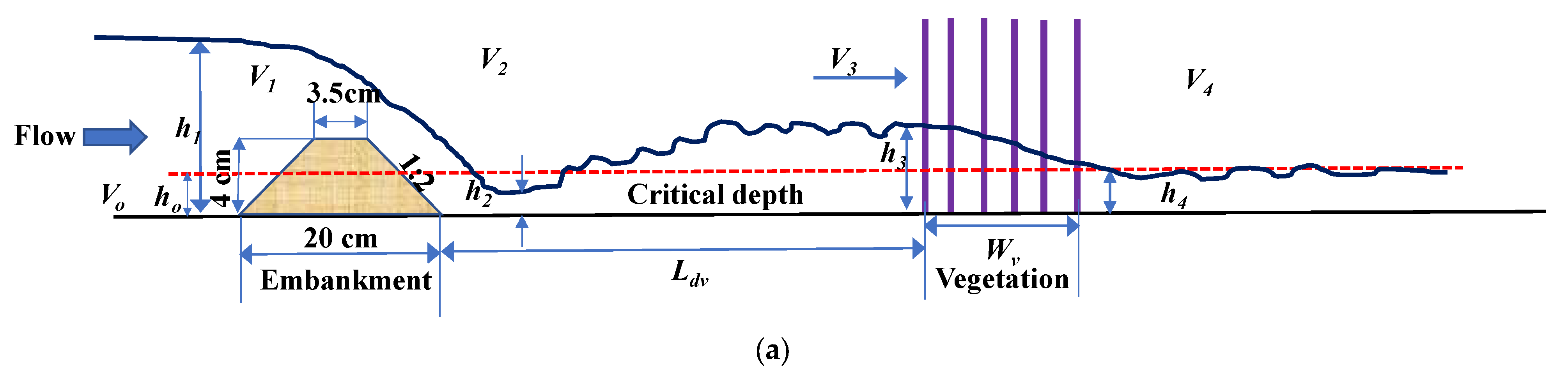
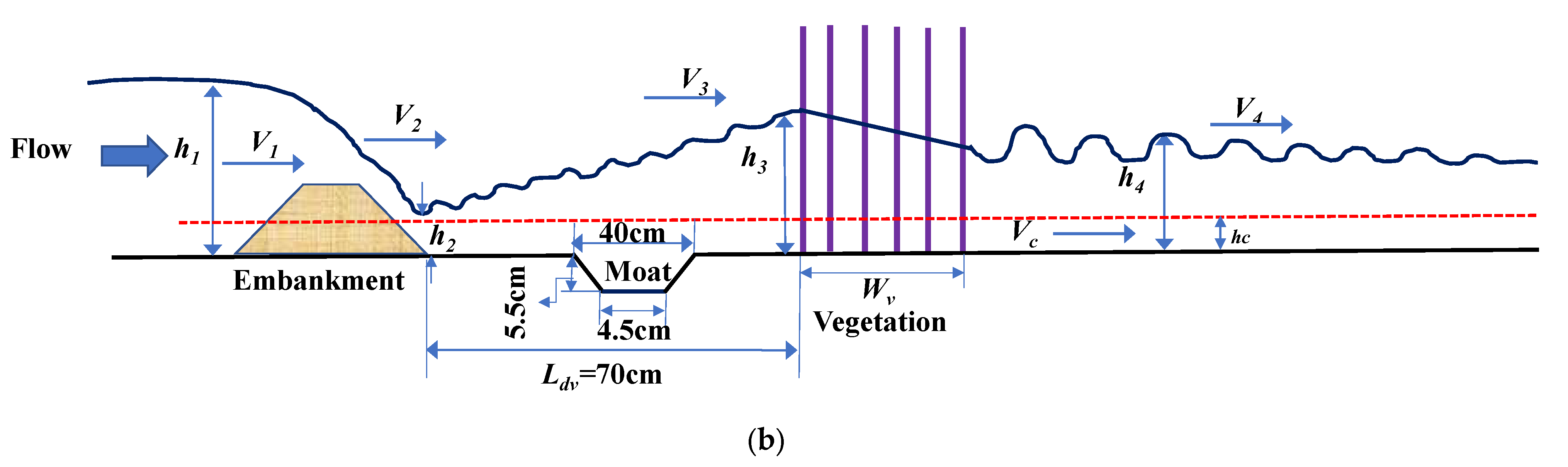
2.1. Flow Resistance of Vegetation

In order to estimate flow resistance for a steady subcritical flow through an emergent vegetation patch, the summation of all the forces on the upstream (F1), downstream (F2), and inside the vegetation patch (F3) can be found. In a two-dimensional flow, the forces F1 and F2 are the hydrodynamic forces acting on the upstream and downstream faces of vegetation, respectively, while F3 is the product of the mass of water flowing per second and change in velocity, which is the vegetation resistance force acting in the opposite direction to F1 in the control volume section. Figure 1a,b show an example of this process. Authors Liu et al. [36] used a similar method to calculate the drag force acting on rigid vegetation under subcritical conditions. Equations (1) and (2) were used to express the force-balance equation along the x direction in their study, neglecting the side wall and bottom effect, as previous studies have [36]:
ƩF = FD = F1F2F3
and
                                                            F D = n   1 2 γ h 1 2 1 2 γ h 2 2 ρ q V 2 V 1 ,
where FD = Net resistive force caused by the number of stems (n) in staggered strip 1 (SS1 in Figure 1c). The first two rows make the staggered arrangement (strip 1), and the other two are behind the first strip [37]. Hence, maximum force and corresponding velocity are applied on the first strip of the vegetation arrangement, and the vegetation in other strips has a lower velocity and drag force, as also observed in previous studies [38]. Therefore, the number of vegetation elements (n) in strip 1 is multiplied by F1, F2, and F3 (Equation (2)), γ = specific volume of water (0.001 m3/kg), = density of water (1000 kg/m3), q = specific discharge (m2/s), i.e., the discharge per unit width, h1 and h2 are the water depths on the upstream and downstream side of vegetation, respectively, yi is the water depth inside the vegetation patch of the ith row, and V1 and V2 are the velocities on the upstream and downstream side of the vegetation patch, respectively. The drag force in the stream-wise direction for the vegetation stem can be calculated by Equation (3), which was also used previously [12,14].
F D = C B D ρ A f V v 2 2 ,
Replacing the drag force in Equation (3) with that from Equation (2), Equation (4) is obtained, for calculating CBD as shown:
C B D = 1 2 γ h 1 2 1 2 γ h 2 2 ρ q v 2 v 1 ρ A f v v 2 2 ,
where Vv is the average pore velocity is close to the actual approach velocity, calculated from the measured flow discharges and λ, i.e.; V v = Q b h 1 λ   a n d   λ = π 2 3   d 2 s 2 , where Q = flow discharge, B = channel width, h = flow depth, s = center-to-center distance between the vegetation stems (Figure 1c), λ = average solid fraction defined as the fraction of the stem-occupied bed area, which represents the density of vegetation [3,15], and Af = the frontal area of each row of vegetation. Equation (4) is used to calculate CBD for all the cases presented in Table 1.

2.2. Dimensional Analysis

In this study, some basic physical quantities affecting the bulk drag coefficient were determined as (Equation (5))
CBD = f1 (ho, Vo, h1, V1, h2, V2, Af, d, υ, Re, Wv, λ)
where ho = the depth of flow without any model placed in the channel, Vo = the depth average velocity without any model placed in the channel, Wv = the width of the vegetation patch, Re = Vv d/υ is the Reynolds number, where Vv is the average flow velocity through the vegetation, d is the diameter of each cylinder used to simulate the vegetation, and υ is the kinematic viscosity of water (1.004 × 10⁻⁶ m2/s), which is the ratio of the viscosity of water to the density of water, and λ = density of vegetation.

2.3. Flow Conditions

The paper utilized Equation (4) to calculate the bulk drag coefficient (CBD) for different flood defense systems. The experimental setup involved two steps. In the first step, the flume was run without any model to record the initial conditions of flow depth (ho) and depth-averaged velocity (Vo). In the second step, the models were placed in the flume, and different cases were tested to calculate CBD. These cases included embankment with vegetation of density λ1 (EVλ1), embankment with vegetation of density λ2 (EVλ2), embankment and moat with vegetation of density λ1 (EMVλ1), and embankment and moat with vegetation of density λ2 (EMVλ2). Moreover, the flow structure of OV, EV, and EMV are shown in Figure 1a–c and Figure 2a,b, and the experimental setup is shown in Figure 3a–c. The study considered two densities of vegetation, i.e., 0.025 (OVλ1) and 0.062 (OVλ2). The Froude numbers considered were 0.40, 0.44, 0.50, 0.57, 0.60, 0.63, and 0.65, with corresponding depths of flow of 4.5 cm, 5.3 cm, 6.8 cm, 7.1 cm, 7.7 cm, 8.2 cm, and 8.5 cm, respectively. The paper measured flow (Q) with an electromagnetic flow meter attached to the channel, and depth-average velocity (V) was calculated by the relation Q = AV. The depth was measured using a rail-mounted adjustable point gauge with the least count of 1 mm. The bed slope of the channel was considered negligible, and the physical modeling scale of 1:100 was used for all the cases mentioned in Table 1.

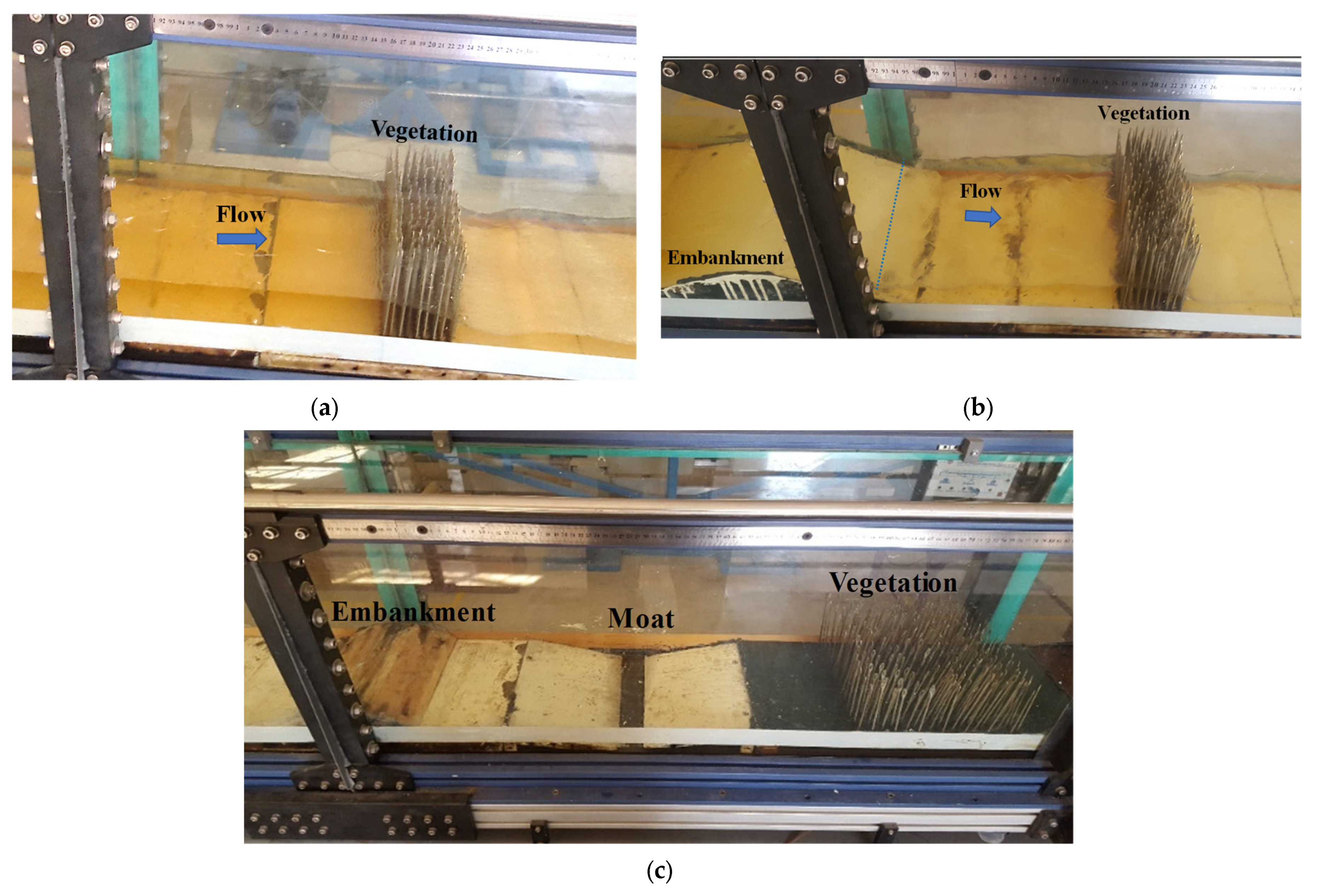
2.4. Vegetation Conditions

Previously, the drag coefficient was calculated by placing flood defense models in an open channel flume of various dimensions (length × width) e.g., 15 m × 0.3 m [39], 3 m × 0.1 m [1], 4.3 m × 0.3 m [40] and 10 m × 0.41 m [41]. The rectangular glass flume used in the current study was 10 m long, 0.5 m deep, and 0.31 m wide. The rigid vegetation was modeled as steel rods embedded in a wooden bed, which was placed inside the flume at a right angle to the flow direction, covering almost the full width of the channel. Two different values of vegetation density (λ) were used to examine their effects, with densities of 0.025 and 0.062, and the spacing between vegetation elements in the cross-stream direction of the flume was 1.88 cm and 1.25 cm, respectively. The diameter of vegetation used for all cases is 0.3 cm. Previous studies have used open-channel flumes of various dimensions to calculate the drag coefficient by placing flood defense models. The width of vegetation (Wv) was calculated by considering the thickness of vegetation dn = 180 No.cm, where d n = 2 D 2 3   W v   ×   s   ×   10 2 , which is the cumulative diameter of trees and is defined as the product of the diameter of trees and the number of trees in a rectangle with a frontage of unit length along the bank of the river and depth equal to the width of vegetation (Wv); the same formula has been used in the past [37]. The selected vegetation pattern, Eucalyptus trees in a staggered arrangement, was based on their average height and diameter in the ecological zone of Punjab province, Pakistan [42], and the use of steel rods as a model is consistent with the 1:100 scale used in the study. Previous research has shown that the drag force behavior is different in grid and staggered vegetation patterns, with some studies finding that staggered arrangements result in higher drag forces and greater effectiveness than grid arrangements [43,44]. Therefore, the staggered arrangement was chosen for the current study.

2.5. Frontal Area of Trees (Af)

To calculate the frontal area of trees, the current study followed the approach used by Liu et al. [36], which involves considering the diameter of stems, the frontal area of stems, and the number of stems. The frontal area is defined as the sum of all the areas covered by the water depth in front of each row of vegetation patches. The equation used to calculate the frontal area of trees is:
A f = d   n j × h j + n k × h k
where nj and nk are the number of vegetation elements in odd and even rows, hj and hk are the depths of flow in front of odd and even rows, respectively, and d is the diameter (0.3 cm) which is kept constant for all the cases mentioned in Table 1. The water depth Af and h2 were measured by a rail-mounted point gauge, and the flow depths in front of each row inside the vegetation patch were calculated by interpolation. Due to the staggered arrangement of the vegetation, the number of vegetation elements in even rows (nk) is nj − 1.

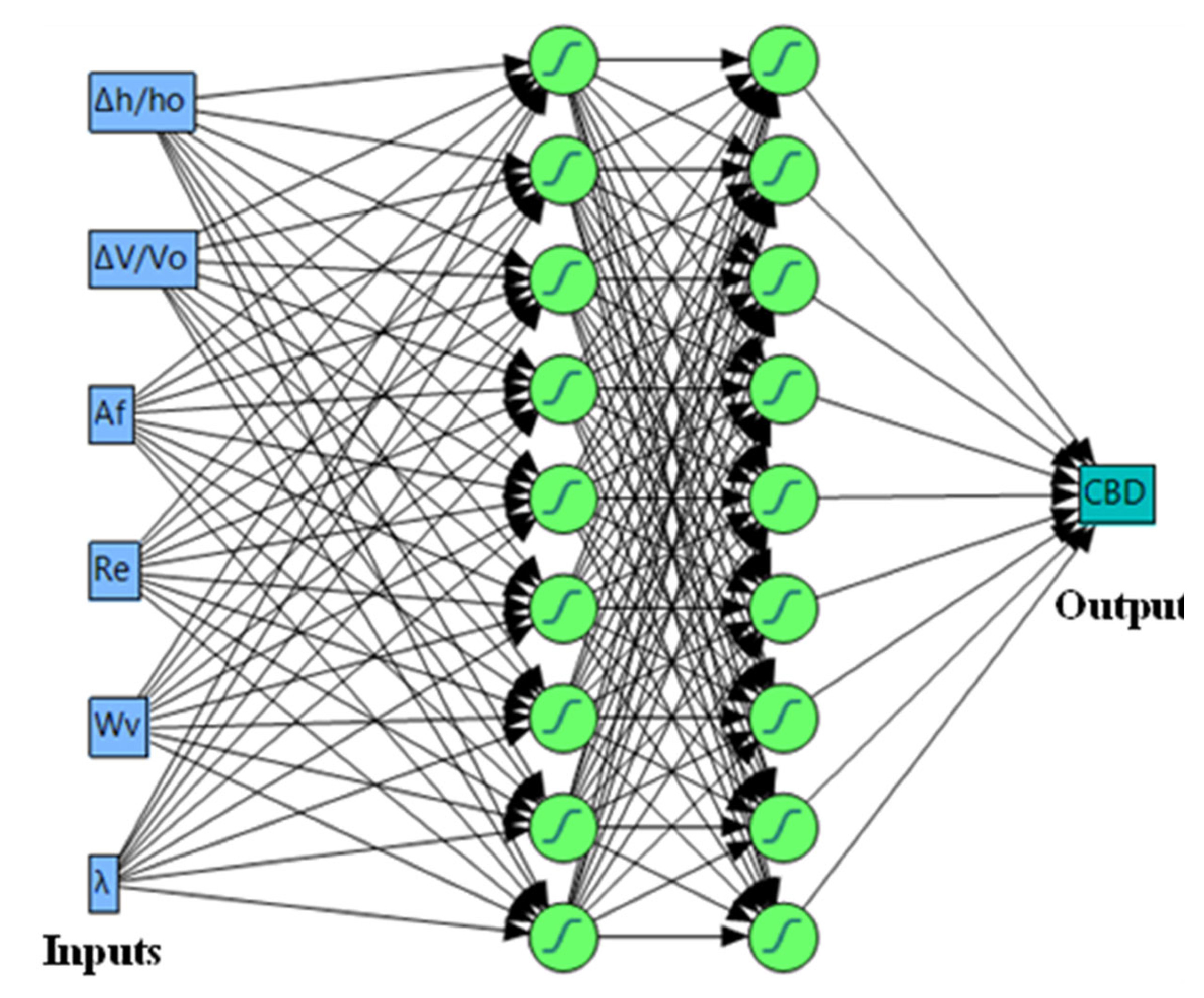
2.6. Artificial Neural Network (ANN)

Artificial neural networks (ANNs) are a type of artificial intelligence that simulates the function of human neurons [45]. ANNs have become increasingly popular for hydrologic modeling and solving problems in engineering and other applied sciences [46]. In this study, five ANN models were tested to determine the best model for predicting CBD, with the input and output values presented in Table 2. While some previous studies have used only training and validation sections for processing ANN models [47,48], others have included training, testing, and validation sections [49,50]. For this study, 67% of the experimentally obtained data were used for validation, while the remaining 33% were used for training the ANN models. The results of the best model are discussed in the parametric study section below. The multilayer perceptron (MLP) is a feed-forward network with layers of neurons that include input, hidden, and output layers. Neurons in the input layer buffer input signals to allocate to neurons in the hidden layer. The flow chart of the feed-forward ANN model is shown in Figure 4.

2.7. Model Performance Evaluation Criteria

The performance of the developed ANN models was tested by statistical error measures, including the coefficient of determination (R2), root mean square error (RMSE), the sum of square error (SSE), the Nash–Sutcliffe model efficiency (NSE), and the mean absolute error (MAE). The formulae of R2, RMSE, SSE, NSE, and MAE are given in Equations (7)–(11).
R 2 = i = 1 n ( C i C ¯ ) ( C i C ¯ ) 2 i = 1 n ( C i C ¯ ) 2 i = 1 n ( C i C ¯ ) 2 ,
The literature indicates that the value of R2 ranges from 0 to 1, where the value 0 implies no correlation and a value of 1 suggests that the model can explain all of the observed variance [48].
R M S E = i = 1 n C i C i 2 n ,
The root mean square error, RMSE, evaluates how closely the predictions match experimental observations; values may range from 0 (perfect fit) to +∞ (no fit) based on the relative range of the data [48].
S S E = i = 1 n C i + C ¯ 2 ,
The sum of squares error (SSE) is a statistical metric used to identify the dispersion of data and how well the data can fit the model. The value of SSE should be a minimum [51].
N S E = 1 i = 1 n C i C i 2 i = 1 n ( C i C ¯ ) 2 ,
The Nash–Sutcliffe efficiency, NSE, measures the model’s ability to predict variables different from the mean and gives the proportion of the initial variance accounted for by the model, where NSE ranges from 1 (perfect fit) to −∞. Values less than zero indicate that the observation means would be a better predictor than the model [48]. An NSE value ranging from 0.75 to 1.0 can be categorized as ‘very good’ [52].
M A E = i = 1 n C i C i n ,
The mean absolute error, MAE, measures the difference between observed and modeled results [48], where C i and C i represent the experimental CBD and computed CBD, C ¯ , (by the ANN) C ¯ represents the average experimental CBD and average computed CBD, and n = no. of observations.

3. Results

3.1. Experimental Results of Bulk Drag Coefficient (CBD)

The experimental bulk drag coefficient was calculated using Equation (4). In the current study, two variables, i.e., density and Reynold’s number, were considered as previously described. Based on these two variables, Equation (12) was developed by regression analysis to calculate CBD within the selected range of λ and Rd for OVλ1 and OVλ2.
C B D = 232 . 75 λ 0.147 R d 0.68 ,
The results of Equation (4) show that the calculated average values of CBD for OVλ1 and OVλ2 were 1.41 and 1.61, respectively, whereas the computed average values of CBD for OVλ1 and OVλ2 were 1.45 and 1.65, respectively. The relation between the calculated values (by Equation (4)) and computed values (by Equation (12)) of CBD is shown in Figure 5a. The R2 values for OVλ1 and OVλ2 were 0.80 and 0.87, respectively, as shown in Figure 5b.
The bulk drag coefficient of vegetation (CBD) usually represents the resistance to flow. CBD can be varied in the case of any structure on the upstream or downstream side of the vegetation. Equation (13) was developed by means of regression analysis to calculate the bulk drag coefficient for EVλ1 and EVλ2 within the selected range of λ and Rd.
C B D = 247.151 λ 0.168 R d 0.70 ,
By using Equation (4), CBD was calculated against the composite defense system’s different values of λ and Rd. Two cases of composite defense systems was tested, i.e., embankment with vegetation of density 0.025 (EVλ1) and embankment with vegetation of density 0.062 (EVλ2). It was found that the calculated value of CBD was decreased by increasing Reynold’s number and increased by increasing λ, as shown in Figure 5a. As a result, the calculated average values of CBD for EVλ1 and EVλ2 were 1.26 and 1.46, respectively. The drag coefficient values for EVλ1 and EVλ2 were also calculated using Equation (4).
The comparison between the calculated values (Equation (4)) and the computed values (Equation (13)) of CBD showed a close relationship, as the value of R2 was 0.97 in both cases, as shown in Figure 5b. The computed average values of CBD for EVλ1 and EVλ2 were 1.41 and 1.65, respectively.
Similarly, the drag coefficient of vegetation (CBD) was calculated using Equation (4) for the composite defense system in the sequence of the embankment, moat/depression, and the vegetation of variable densities. The calculated average values of CBD for EMVλ1 and EMVλ2 were 1.16 and 1.29, respectively, based on these two variables, i.e., density and Reynolds number. Finally, Equation (14) was developed by regression analysis to compute the bulk drag coefficient for the EMVλ1 and EMVλ2 cases within the selected range of variables. The computed average values of CBD for EMVλ1 and EMVλ2 were 1.16 and 1.30, respectively.
C B D = 174.164 λ 0.126 R d 0.68
The graphical representation between the calculated values (Equation (4)) and the computed values (Equation (14)) showed a close relationship, as the R2 values were 0.96 and 0.95 for EMVλ1 and EMVλ2, respectively, as shown in Figure 5b. A summary of CBD values calculated (Equation (4)) and computed (Equations (12)–(14)) is presented in Table 3.

3.2. Computed Results of Bulk Drag Coefficient (CBD) by ANN Model

To predict CBD, five different ANN models were tested to optimize the best model. Each ANN model contained two layers, which were kept constant for all models. However, the number of neurons in each layer varied. The result shows that the performance of the ANN9 model, i.e., with nine neurons in each layer, was the best among all models. As discussed previously, the performance of models was judged by various performance indicators. Therefore, the value of R2 and NSE of the ANN9 model (for testing and validation) was the highest, showing the best performance, as presented in Table 4 and Figure 6a,b.
Moreover, the values of SSE, RMSE, and MAE of the ANN9 model (for testing and validation) were the lowest among all models, as shown in Table 4 and presented in Figure 6c–e. The relationship between experimental and computed values (from the ANN9 model) is shown in Figure 6f, showing a good relationship as the value of R2 was 0.99, which is close to unity. In Figure 6a–e, “T” and “V” represent testing and validation, respectively. Previously, the performance of various prediction models was also tested by various authors by constructing Taylor’s diagram [53,54], which was also adopted in the current study. Taylor’s diagram shows the relationship between standard deviation, correlation coefficient (R2), and root mean square error (RMSE), as shown in Figure 7a,b. It was observed that the standard deviation and RMSE values of ANN9 were performed at least as well as or better than the other ANN models, as well as the regression model (RM) for both training and validation sections. On the other hand, the values of R2 of all the ANN models were in the range of 0.970–0.999, which is higher than 0.920 for the regression model. Therefore, the ANN models, including ANN9, had a better overall performance compared to the regression model, as they had higher R2 values and lower RMSE and standard deviation values.

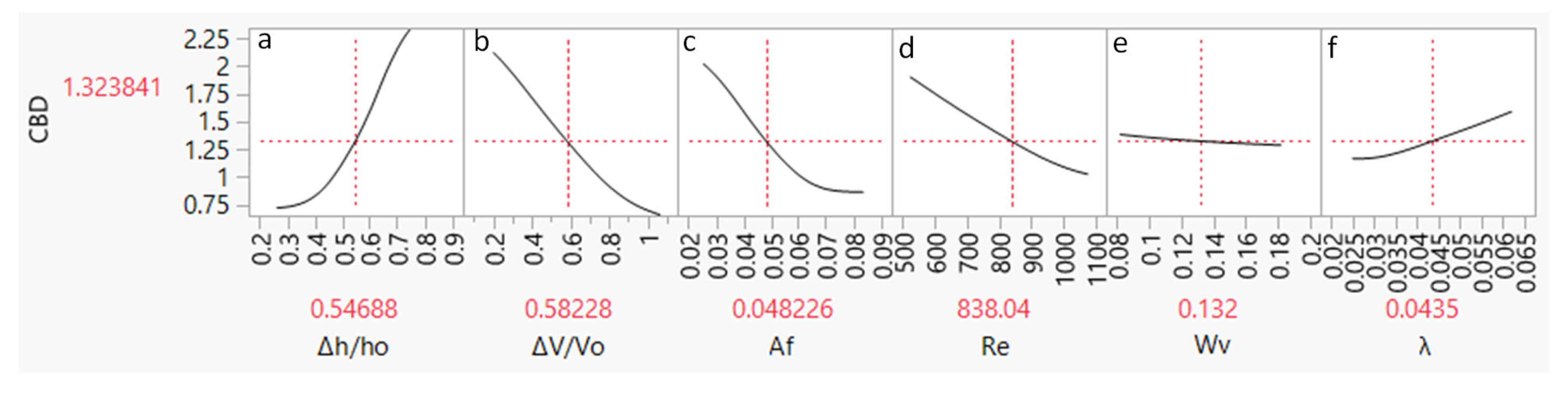
3.3. Prediction Results of CBD against Various Parameters

The predicted values of the bulk drag coefficient against all variables are shown in Figure 8 (generated by the software). The prediction results show that CBD increased by increasing the variables Δh/ho and λ; however, the reverse relation is observed for ΔV/Vo, Af, Re, and Wv. Maximum variation in CBD is observed against Δh/ho and minimum against Wv. Hence, the variables ΔV/Vo, Af, Re, and Wv should decrease the bulk drag coefficient. The drag coefficient of vegetation may lead to tree breakage. Implementing this study’s analysis framework and results in hydraulic engineering practice can help the planning and management divisions avoid tree breakage and efficiently slow the flow during extreme hydrologic events and floods.

4. Discussion

In previous studies, drag force has been investigated in terms of drag coefficient, using various methods such as the energy-slope method [1], water-surface-slope method [39], and strain gauges [55]. Researchers have experimentally calculated the drag coefficient of vegetation with variable densities (λ) and various configuration patterns. For instance, Ishikawa [39] and James [1] used a staggered pattern of vegetation with densities ranging from 0.00314 to 0.0126 [39] and 0.0035 to 0.0314, respectively. Meanwhile, Tanino and Nepf [14] and Coscarella [56] considered random vegetation patterns with densities ranging from 0.15 to 0.35 and 0.022 to 0.038, respectively.
The study conducted experiments to calculate the bulk drag coefficient (CBD) under subcritical steady-flow conditions for two cases of only vegetation (OV), i.e., OVλ1 and OVλ2 (where λ1 = 0.025 and λ2 = 0.062), placed in a staggered pattern. The calculated values of CBD showed a direct relation with density (λ) and an inverse relation with Reynolds number (Rd), consistent with previous studies [3,5], which also found a similar relationship between drag coefficient and either Froude number [39] or Reynolds number [57]. Various methods have been explored in previous studies to calculate drag force in terms of drag coefficient, with calculated ranges of bulk drag coefficient against different variables of 1.22–1.39 [22], 1.5–4.0 [58], 1.19–1.26 [59], 1.33–2.0 [14], and 1.13–2.05 [60]. The calculated range of CBD in the present study was 1.24–2.18, which agrees well with the results of previous studies.
The study also applied the same method to calculate CBD for a composite defense system comprising four parts, i.e., EVλ1, EVλ2, EMVλ1, and EMVλ2, respectively. The calculated results showed that the combination of an upstream structure reduces the drag coefficient of vegetation because the drag coefficient is shared by both the embankment and vegetation in the composite structure. By placing the embankment upstream of vegetation, the average CBD for EVλ1 and EVλ2 decreased by 10.6% and 11%, respectively.
In a similar vein, the CBD was reduced by 17.73% and 20% for the EMVλ1 and EMVλ2 cases, respectively, when compared to only vegetation. Like previous researchers, we employed regression analysis to develop equations for computing the CBD, taking into account variables such as λ and Rd. The comparison between the computed and calculated results indicates a high level of agreement, as evidenced by an R2 value close to unity. The present study investigated the impact of upstream structures, which has been studied previously. Contemporary engineering practices and research can employ artificial neural networks to forecast various hydraulic parameters.
Previous studies have employed ANN models and gene-expression programming (GEP) to predict the flow resistance of flexible vegetation in laboratory channels and compared the results with regression models. The ANN model was found to perform better than GEP and regression analysis [61]. In the present study, similar results were obtained, where the performance of the ANN model was superior to that of the regression models. Five ANN models were evaluated with different hidden layers and varying numbers of neurons, and the best-performing model was found to be the one with two hidden layers and nine neurons (ANN9) in each layer. The performance of the ANN models was assessed using five performance indicators, and ANN9 was found to have the highest R2 and NSE values and the lowest RMSE, SSE, and MAE values for both training and validation. The comparison between regression models and the ANN9 model showed that the R2 value for ANN9 was 0.99 and 0.98 for training and validation, respectively, while the maximum R2 for regression analysis was 0.97 for both EVλ1 and EVλ2. The regression model performance for EMVλ1 and EMVλ2 was also satisfactory with R2 values of 0.96 and 0.95, respectively. The regression model performance for OVλ1 and OVλ2 was acceptable, with R2 values of 0.80 and 0.87, respectively. Nonetheless, the ANN9 model was found to be the best among all the models.
To evaluate the performance of the ANN models and compare them with regression models, Taylor’s diagram was constructed, which has been previously adopted by other researchers. The diagram confirms that the ANN9 model outperformed both other ANN and regression models. The parametric study conducted shows that CBD increases with variables such as Δh/ho and λ, while variables such as ΔV/Vo, Af, Re, and Wv decrease the bulk drag coefficient, with the minimum variation observed for Wv. The study highlights the potential risk of tree breakage due to the drag coefficient of vegetation, and planning and management divisions should consider the parametric study results to prevent tree breakage during high floods. It is important to note that the experimental setup used in the study, with an embankment model and moat/depression models upstream of the vegetation, may not be representative of all natural environments where vegetation and upstream structures exist. Therefore, the findings of the study may have limited applicability to other environments. However, the study can serve as a baseline to analyze drag force on vegetation in composite defense systems that incorporate hard and soft solutions. As such, the effect of upstream structures should be considered in a composite defense system, and future research should also investigate the effect of downstream structures on the drag coefficient of vegetation.

5. Conclusions

Based on the results of the bulk drag coefficient through vegetation and the effect of an upstream structure, the following conclusions were drawn:
  • The calculated CBD for OVλ1 and OVλ2 showed a direct relationship with vegetation density (λ) and an inverse relationship with Reynolds number (Rd). The calculated ranges of CBD for OVλ1 and OVλ2 were 1.24–1.84 and 1.40–2.18, respectively, with average CBD values of 1.41 and 1.61, respectively.
  • The average CBD values for EVλ1 and EVλ2, which represent composite defense cases, were decreased by 10.6% and 11% compared to OVλ1 and OVλ2, respectively. As a result, the calculated average CBD values for EVλ1 and EVλ2 were 1.26 and 1.41, respectively.
  • The average CBD values for EMVλ1 and EMVλ2, which also represent composite defense cases, were decreased by 17.73% and 20% compared to OVλ1 and OVλ2, respectively. The calculated average CBD values for EMVλ1 and EMVλ2 were 1.16 and 1.29, respectively.
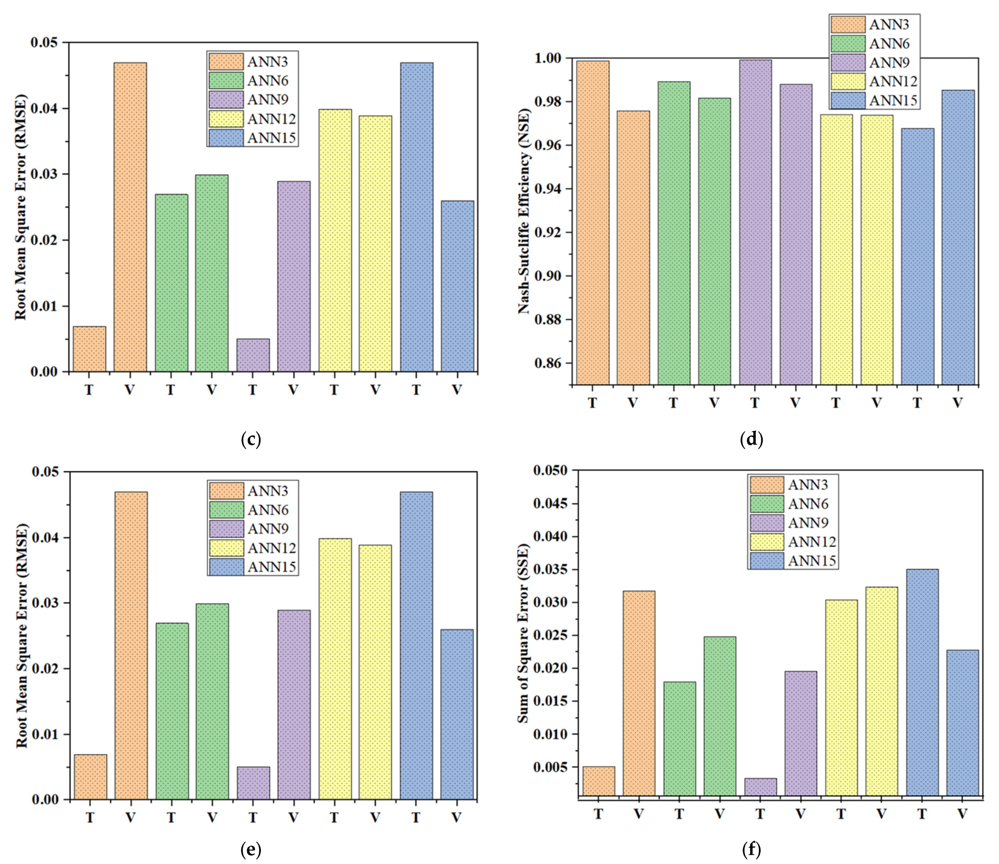
  • The ANN9 model provided the best performance among the five ANN models, with the highest R2 and NSE values and the lowest RMSE, SSE, and MAE values.
  • When compared to the prediction of CBD, the ANN9 model outperformed the regression models tested using Taylor’s diagram.
The results of the current study provide insights into the performance comparison of different models, including ANN models and regression models, in predicting a certain variable. This information can be used by researchers to select the appropriate model for their own research based on the performance criteria of the model. The current study highlights the superiority of ANN models, particularly the ANN9 model, over the regression model in terms of standard deviation, correlation coefficient (R2), and root mean square error (RMSE). This information can be used by researchers who are working on similar problems and can benefit from the use of ANN models.

Author Contributions

A.A., A.R.G. and G.A.P.; methodology: A.A., A.R.G. and G.A.P.; formal analysis: A.A., R.F. and S.J.; writing—original draft preparation: A.A., M.V., R.F., G.A.P. and A.R.; visualization: A.A., M.V., R.F. and G.A.P.; supervision: A.R.G. and M.V. All authors have read and agreed to the published version of the manuscript.

Funding

The authors acknowledge the support of HEC Pakistan under the International research support initiative program. No: IRSIP 44 Engg. 07, 1-8/HEC/HRD/2019/10122.

Institutional Review Board Statement

Not applicable.

Informed Consent Statement

Not applicable.

Data Availability Statement

Materials and data used in the present paper are available under request to the corresponding author.

Acknowledgments

This study was funded by University of Engineering and Technology, Taxila, Pakistan. The authors acknowledge Ghufran Ahmed Pasha and Rashid Farooq for their useful comments and great help during whole of this research.

Conflicts of Interest

The authors declare no conflict of interest.

References

  1. James, C.S.; Birkhead, A.L.; Jordanova, A.A.; O’sullivan, J.J. Flow resistance of emergent vegetation. J. Hydraul. Res. 2004, 42, 390–398. [Google Scholar] [CrossRef]
  2. Luhar, M.; Rominger, J.; Nepf, H. Interaction between flow, transport and vegetation spatial structure. Environ. Fluid Mech. 2008, 8, 423–439. [Google Scholar] [CrossRef]
  3. Cheng, N.; Nguyen, H.T. Hydraulic Radius for Evaluating Resistance Induced by Simulated Emergent Vegetation in Open-Channel Flows. J. Hydraul. Eng. 2011, 137, 995–1004. [Google Scholar] [CrossRef]
  4. Aboueian, J.; Sohankar, A.; Rastan, M.R.; Ghodrat, M. An experimental study on flow over two finite wall-mounted square cylinders in a staggered arrangement. Ocean Eng. 2021, 240, 109954. [Google Scholar] [CrossRef]
  5. Wang, W.; Peng, W.; Huai, W.; Katul, G.G.; Liu, X. Friction factor for turbulent open channel flow covered by vegetation. Sci. Rep. 2019, 9, 5178. [Google Scholar] [CrossRef] [Green Version]
  6. Hui, E.Q.; Hu, X.E.; Jiang, C.B.; Zhu, Z.D. A study of drag coefficient related with vegetation based on the flume experiment. J. Hydrodyn. Ser. B 2010, 22, 329–337. [Google Scholar] [CrossRef]
  7. Yang, S.; Balachandar, R. Determination of Velocity Distribution and Flow Resistance in Vegetated Channel Flows; University of Wollongong Australia: Wollongong, NSW, Australia, 2016; pp. 2211–2218. [Google Scholar]
  8. Ahmed, A.; Ghumman, A.R. Experimental Investigation of Flood Energy Dissipation by Single and Hybrid Defense System. Water 2019, 11, 1971. [Google Scholar] [CrossRef] [Green Version]
  9. Farooq, R.; Ahmad, W.; Hashmi, H.N.; Saeed, Z. Computation of Momentum Transfer Coefficient and Conveyance Capacity in Asymmetric Compound Channel. Arab. J. Sci. Eng. 2016, 41, 4225–4234. [Google Scholar] [CrossRef]
  10. Baptist, M.; Babovic, V.; Rodriguez Uthurburu, J.; Keijzer, M.; Uittenbogaard, R.; Mynett, A.; Verwey, A. On inducing equations for vegetation resistance. J. Hydraul. Res. 2007, 45, 435–450. [Google Scholar] [CrossRef]
  11. Huthoff, F.; Augustijn, D.C.M.; Hulscher, S.J.M.H. Analytical solution of the depth-averaged flow velocity in case of submerged rigid cylindrical vegetation. Water Resour. Res. 2007, 43, 1–10. [Google Scholar] [CrossRef] [Green Version]
  12. Panigrahi, K.; Khatua, K.K. Prediction of velocity distribution in straight channel with rigid vegetation. Aquat. Procedia 2015, 4, 819–825. [Google Scholar] [CrossRef]
  13. Järvelä, J. Determination of flow resistance of vegetated channel banks and floodplains. In River Flow; Helsinki University of Technology: Espoo, Finland, 2002; pp. 311–318. [Google Scholar]
  14. Tanino, Y.; Nepf, H.M. Laboratory investigation of mean drag in a random array of rigid, emergent cylinders. J. Hydraul. Eng. 2008, 134, 34–41. [Google Scholar] [CrossRef]
  15. Cheng, N.-S. Calculation of Drag Coefficient for Arrays of Emergent Circular Cylinders with Pseudofluid Model. J. Hydraul. Eng. 2013, 139, 602–611. [Google Scholar] [CrossRef]
  16. Huai, W.; Wang, W.; Hu, Y.; Zeng, Y.; Yang, Z. Analytical model of the mean velocity distribution in an open channel with double-layered rigid vegetation. Adv. Water Resour. 2014, 69, 106–113. [Google Scholar] [CrossRef]
  17. Pasha, G.A.; Tanaka, N. Undular hydraulic jump formation and energy loss in a flow through emergent vegetation of varying thickness and density. Ocean Eng. 2017, 141, 308–325. [Google Scholar] [CrossRef]
  18. Wieselsberger, C. New Data on the Laws of Fluid Resistance; NASA: Washington, DC, USA, 1922.
  19. Mellado, J.P.; Wang, L.; Peters, N. Gradient trajectory analysis of a scalar field with external intermittency. J. Fluid Mech. 2009, 626, 333–365. [Google Scholar] [CrossRef]
  20. Su, H.B.; Schmid, H.P.; Vogel, C.S.; Curtis, P.S. Effects of canopy morphology and thermal stability on mean flow and turbulence statistics observed inside a mixed hardwood forest. Agric. For. Meteorol. 2008, 148, 862–882. [Google Scholar] [CrossRef]
  21. Sonnenwald, F.; Stovin, V.; Guymer, I. Estimating drag coefficient for arrays of rigid cylinders representing emergent vegetation. J. Hydraul. Res. 2018, 57, 591–597. [Google Scholar] [CrossRef] [Green Version]
  22. Suzuki, T.; Arikawa, T. Numerical Analysis of Bulk Drag Coefficient in Dense Vegetation by Immersed Boundary Method. Coast. Eng. Proc. 2011, 1, 48. [Google Scholar] [CrossRef] [Green Version]
  23. Thompson, A.M.; Wilson, B.N.; Hansen, B.J. Shear stress partitioning for idealized vegetated surfaces. Trans. ASAE 2004, 47, 701. [Google Scholar] [CrossRef]
  24. Li, R.M.; Shen, H.W. Effect of tall vegetations on flow and sediment. J. Hydraul. Div. 1973, 99, 793–814. [Google Scholar] [CrossRef]
  25. Fathi-Maghadam, M.; Kouwen, N. Nonrigid, nonsubmerged, vegetative roughness on floodplains. J. Hydraul. Eng. 1997, 123, 51–57. [Google Scholar] [CrossRef]
  26. Armanini, A.; Righetti, M.; Grisenti, P. Direct measurement of vegetation resistance in prototype scale. J. Hydraul. Res. 2005, 43, 481–487. [Google Scholar] [CrossRef]
  27. Wu, F. Characteristics of flow resistance in open channels with non-submerged rigid vegetation. J. Hydrodyn. Ser. B 2008, 20, 239–245. [Google Scholar] [CrossRef]
  28. Wu, F.-C.; Shen, H.W.; Chou, Y.-J. Variation of roughness coefficients for unsubmerged and submerged vegetation. J. Hydraul. Eng. 1999, 125, 934–942. [Google Scholar] [CrossRef] [Green Version]
  29. Muhammad, A.H.; Tanaka, N. Energy Reduction of a Tsunami Current through a Hybrid Defense System Comprising a Sea Embankment Followed by a Coastal Forest. Geosciences 2019, 9, 247. [Google Scholar] [CrossRef] [Green Version]
  30. Zaha, T.; Tanaka, N.; Kimiwada, Y. Flume experiments on optimal arrangement of hybrid defense system comprising an embankment, moat, and emergent vegetation to mitigate inundating tsunami current. Ocean Eng. 2019, 173, 45–57. [Google Scholar] [CrossRef]
  31. Pasha, G.A.; Tanaka, N.; Yagisawa, J.; Achmad, F.N. Tsunami mitigation by combination of coastal vegetation and a backward-facing step. Coast. Eng. J. 2018, 60, 104–125. [Google Scholar] [CrossRef]
  32. Muhammad, M.M.; Yusof, K.W.; Mustafa, M.R.U.; Zakaria, N.A.; Ghani, A.A. Artificial neural network applications for predicting drag coefficient in flexible vegetated channels. J. Telecommun. Electron. Comput. Eng. 2018, 10, 99–102. [Google Scholar]
  33. Smith, J.; Eli, R.N. Neural-network models of rainfall-runoff process. J. Water Resour. Plan. Manag. 1995, 121, 499–508. [Google Scholar] [CrossRef]
  34. Kisi, O.; Shiri, J.; Nikoofar, B. Forecasting daily lake levels using artificial intelligence approaches. Comput. Geosci. 2012, 41, 169–180. [Google Scholar] [CrossRef]
  35. Edossa, D.C.; Babel, M.S. Application of ANN-Based Streamflow Forecasting Model for Agricultural Water Management in the Awash River Basin, Ethiopia. Water Resour. Manag. 2011, 25, 1759–1773. [Google Scholar] [CrossRef]
  36. Liu, X.; Zeng, Y. Drag coefficient for rigid vegetation in subcritical open-channel flow. Environ. Fluid Mech. 2017, 17, 1035–1050. [Google Scholar] [CrossRef]
  37. Pasha, G.A.; Tanaka, N. Critical Resistance Affecting Sub- to Super-Critical Transition Flow by Vegetation. J. Earthq. Tsunami 2019, 13, 1950004. [Google Scholar] [CrossRef]
  38. Anjum, N.; Ghani, U.; Pasha, G.A.; Rashid, M.U.; Latif, A.; Rana, M.Z.Y. Reynolds stress modeling of flow characteristics in a vegetated rectangular open channel. Arab. J. Sci. Eng. 2018, 43, 5551–5558. [Google Scholar] [CrossRef]
  39. Ishikawa, Y.; Mizuhara, K.; Ashida, M. Drag force on multiple rows of cylinders in an open channel. In Grant-in-Aid Research Project Report; Kyushu University: Fukuoka, Japan, 2000. [Google Scholar]
  40. Liu, D.; Hession, C. Flow through Rigid Vegetation Hydrodynamics. Ph.D. Thesis, Virginia Polytechnic Institute and State University, Blacksburg, VA, USA, 2008. [Google Scholar]
  41. Ferreira, R.M.L.; Ricardo, A.M.; Franca, M.J. Discussion of ‘Laboratory investigation of mean drag in a random array of rigid, emergent cylinders’ by Yukie Tanino and Heidi M. Nepf. J. Hydraul. Eng. 2009, 135, 690–693. [Google Scholar] [CrossRef]
  42. Tanvir, M.A.; Siddiqui, M.T.; Shah, A.H. Growth and price trend of Eucalyptus camaldulensis in Central Punjab. Int. J. Agric. Biol. 2002, 4, 344–346. [Google Scholar]
  43. Takemura, T.; Tanaka, N. Flow structures and drag characteristics of a colony-type emergent roughness model mounted on a flat plate in uniform flow. Fluid Dyn. Res. 2007, 39, 694–710. [Google Scholar] [CrossRef]
  44. Bokaian, A.; Geoola, F. Wake-induced galloping of two interfering circular cylinders. J. Fluid Mech. 1984, 146, 383–415. [Google Scholar] [CrossRef]
  45. Khedri, A.; Kalantari, N.; Vadiati, M. Comparison study of artificial intelligence method for short term groundwater level prediction in the northeast Gachsaran unconfined aquifer. Water Sci. Technol. Water Supply 2020, 20, 909–921. [Google Scholar] [CrossRef]
  46. Wunsch, A.; Liesch, T.; Broda, S. Forecasting groundwater levels using nonlinear autoregressive networks with exogenous input (NARX). J. Hydrol. 2018, 567, 743–758. [Google Scholar] [CrossRef]
  47. Tayfur, G.; Singh, V.P. ANN and Fuzzy Logic Models for Simulating Event-Based Rainfall-Runoff. J. Hydraul. Eng. 2006, 132, 1321–1330. [Google Scholar] [CrossRef] [Green Version]
  48. Hu, C.; Wu, Q.; Li, H.; Jian, S.; Li, N.; Lou, Z. Deep learning with a long short-term memory networks approach for rainfall-runoff simulation. Water 2018, 10, 1543. [Google Scholar] [CrossRef] [Green Version]
  49. Almuhaylan, M.R.; Ghumman, A.R.; Al-Salamah, I.S.; Ahmad, A.; Ghazaw, Y.M.; Haider, H.; Shafiquzzaman, M. Evaluating the impacts of pumping on aquifer depletion in arid regions using MODFLOW, ANFIS and ANN. Water 2020, 12, 2297. [Google Scholar] [CrossRef]
  50. Iqbal, M.; Naeem, U.A.; Ahmad, A.; Rehman, H.; Ghani, U.; Farid, T. Relating groundwater levels with meteorological parameters using ANN technique. Meas. J. Int. Meas. Confed. 2020, 166, 108163. [Google Scholar] [CrossRef]
  51. Keskin, M.E.; Terzi, Ö. Artificial Neural Network Models of Daily Pan Evaporation. J. Hydrol. Eng. 2006, 11, 65–70. [Google Scholar] [CrossRef]
  52. Rauf, A.; Ghumman, A.R. Impact assessment of rainfall-runoffsimulations on the flow duration curve of the Upper Indus river-a comparison of data-driven and hydrologic models. Water 2018, 10, 876. [Google Scholar] [CrossRef] [Green Version]
  53. Ghumman, A.R.; Pasha, G.A.; Ahmad, A.; Ahmed, A.; Khan, R.A.; Farooq, R. Simulation of Quantity and Quality of Saq Aquifer Using Artificial Intelligence and Hydraulic Models. Adv. Civ. Eng. 2022, 2022, 5910989. [Google Scholar] [CrossRef]
  54. Samui, T.P.P. Prediction of Rock Strain Using Hybrid Approach of Ann and Optimization Algorithms. Geotech. Geol. Eng. 2022, 40, 4617–4643. [Google Scholar] [CrossRef]
  55. Kothyari, U.C.; Hayashi, K.; Hashimoto, H. Drag coefficient of unsubmerged rigid vegetation stems in open channel flows. J. Hydraul. Res. 2009, 47, 691–699. [Google Scholar] [CrossRef]
  56. Coscarella, F.; Penna, N.; Ferrante, A.P.; Gualtieri, P.; Gaudio, R. Turbulent flow through random vegetation on a rough bed. Water 2021, 13, 2564. [Google Scholar] [CrossRef]
  57. White, F.M. Viscous Fluid Flow; McGraw-Hill: New York, NY, USA, 1991. [Google Scholar]
  58. Tinoco, R.O.; Cowen, E.A. The direct and indirect measurement of boundary stress and drag on individual and complex arrays of elements. Exp. Fluids 2013, 54, 1509. [Google Scholar] [CrossRef]
  59. Stoesser, T.; Kim, S.J.; Diplas, P. Turbulent flow through idealized emergent vegetation. J. Hydraul. Eng. 2010, 136, 1003–1017. [Google Scholar] [CrossRef]
  60. Liu, X.G.; Zeng, Y.H. Drag coefficient for rigid vegetation in subcritical open channel. Procedia Eng. 2016, 154, 1124–1131. [Google Scholar] [CrossRef] [Green Version]
  61. Muhammad, M.M.; Yusof, K.W.; Mustafa, M.R.U.; Zakaria, N.A.; Ghani, A.A. Prediction models for flow resistance in flexible vegetated channels. Int. J. River Basin Manag. 2018, 16, 427–437. [Google Scholar] [CrossRef]
Figure 1. (a,b) offer distinct conceptual illustrations of the theoretical model for deriving the bulk vegetation drag coefficient, CBD; (c) is the theoretical arrangement of vegetation in strips.
Hydrology 10 00073 g001
Figure 2. Illustration of free-water surface characteristic profiles for the cases of: (a) embankment and vegetation (EV) model; (b) embankment, moat, and vegetation (EMV) model.
Hydrology 10 00073 g002aHydrology 10 00073 g002b
Figure 3. Illustration of the test section of the different experiments assessed herein: (a) only vegetation (OV); (b) embankment and vegetation (EV) model; (c) embankment, moat, and vegetation (EMV) model.
Hydrology 10 00073 g003
Figure 4. Depiction of the architecture of the feed-forward ANN model.
Hydrology 10 00073 g004
Figure 5. (a) Experimental CBD vs. Re and (b) relation between experimental and computed CBD.
Hydrology 10 00073 g005
Figure 6. Performance indicators for ANN models: (a) R2; (b) NSE; (c) RMSE; (d) SSE; (e) MAE; and (f) comparison b/w experimental and computed CBD.
Hydrology 10 00073 g006aHydrology 10 00073 g006b
Figure 7. Taylor’s diagram showing the relationship between standard deviation, correlation coefficient, and root mean square error (represented with blue lines) for CBD; (a) Training and (b) Validation.
Hydrology 10 00073 g007
Figure 8. Predicted values of the bulk drag coefficient against variables; (a) Δh/ho, (b) ΔV/Vo, (c) Af, (d) Re, (e) Wv and (f) λ.
Hydrology 10 00073 g008
Table 1. Presentation of the hydraulic parameters for the conducted experiments.
Case IDInitial Froude
(Fro)
Initial Water Depth (ho)
[cm]
Density
(λ)
Vegetation Width (Wv) [cm]dsRe Range
OVλ10.40, 0.44, 0.50, 0.57,
0.60, 0.63, 0.65
4.5, 5.3, 6.8, 7.1,
7.7, 8.2, 8.5
0.02518.40.31.25553–996
OVλ20.40, 0.44, 0.50, 0.57,
0.60, 0.63, 0.65
4.5, 5.3, 6.8, 7.1,
7.7, 8.2, 8.5
0.0628.20.31.88524–1004
EVλ10.40, 0.44, 0.50, 0.57,
0.60, 0.63, 0.65
4.5, 5.3, 6.8, 7.1,
7.7, 8.2, 8.5
0.02518.40.31.25524–1029
EVλ20.40, 0.44, 0.50, 0.57,
0.60, 0.63, 0.65
4.5, 5.3, 6.8, 7.1,
7.7, 8.2, 8.5
0.0628.20.31.88599–1064
EMVλ10.40, 0.44, 0.50, 0.57,
0.60, 0.63, 0.65
4.5, 5.3, 6.8, 7.1,
7.7, 8.2, 8.5
0.02518.40.31.25524–1037
EMVλ20.40, 0.44, 0.50, 0.57,
0.60, 0.63, 0.65
4.5, 5.3, 6.8, 7.1,
7.7, 8.2, 8.5
0.0628.20.31.88559–1073
Table 2. Presentation of ANN model inputs and outputs.
ANN Model IDInput VariablesNo. of Hidden LayersNo. of Neurons in Each LayerOutput
ANN3Δh/ho, ΔV/Vo, Af, Re, Wv, λ23CBD
ANN6Δh/ho, ΔV/Vo, Af, Re, Wv, λ26CBD
ANN9Δh/ho, ΔV/Vo, Af, Re, Wv, λ29CBD
ANN12Δh/ho, ΔV/Vo, Af, Re, Wv, λ212CBD
ANN15Δh/ho, ΔV/Vo, Af, Re, Wv, λ215CBD
Table 3. Presentation of the hydraulic parameters for the conducted experiments.
Sr. No.Case NameEquation Used (Calculated)Equation Used
(Computed)
CBD
Range (Calculated)
CBD
Range
(Computed)
Average CBD
(Calculated)
Average CBD
(Computed)
1OVλ1Equation (4) C B D =
232.75 λ 0.147 R d 0.68
1.10–1.741.24–1.841.411.45
2OV λ2Equation (4) C B D =
232.75 λ 0.147 R d 0.68
1.31–1.961.40–2.181.611.65
3EV λ1Equation (4) C B D =
247.15 λ 0.168 R d 0.70
1–1.631.18–1.801.261.41
4EV λ2Equation (4) C B D =
247.15 λ 0.168 R d 0.70
1.2–1.791.41–2.121.461.65
5EMV λ1Equation (4) C B D =
174.164 λ 0.126 R d 0.68
0.9–1.500.96–1.481.161.16
6EMV λ1Equation (4) C B D =
174.164 λ 0.126 R d 0.68
1.11–1.611.10–1.651.291.30
Table 4. Performance evaluation of the assessed ANN models.
ANN3ANN6ANN9ANN12ANN15
TVTVTVTVTV
R20.9990.9760.9990.9810.9990.9880.9800.9700.9800.970
RMSE0.0070.0470.0270.0300.0050.0290.0400.0390.0470.026
SSE0.0020.0420.0180.0270.0010.0170.0300.0610.0130.084
NSE0.9990.9760.9900.9821.0000.9880.9740.9740.9680.985
MAE0.0050.0320.0180.0250.0030.0200.0300.0320.0350.023
Disclaimer/Publisher’s Note: The statements, opinions and data contained in all publications are solely those of the individual author(s) and contributor(s) and not of MDPI and/or the editor(s). MDPI and/or the editor(s) disclaim responsibility for any injury to people or property resulting from any ideas, methods, instructions or products referred to in the content.

