Article

Utilizing NDWI, MNDWI, SAVI, WRI, and AWEI for Estimating Erosion and Deposition in Ping River in Thailand

by
Jeerapong Laonamsai
1,2,*,
Phongthorn Julphunthong
1,3,
Thanat Saprathet
4,
Bounhome Kimmany
5,
Tammarat Ganchanasuragit
6,
Phornsuda Chomcheawchan
1 and
Nattapong Tomun
7
1
Department of Civil Engineering, Faculty of Engineering, Naresuan University, Phitsanulok 65000, Thailand
2
Water Resources Research Center, Faculty of Engineering, Naresuan University, Phitsanulok 65000, Thailand
3
Research Center for Academic Excellence in Applied Physics, Faculty of Science, Naresuan University, Phitsanulok 65000, Thailand
4
Department of Water Resources, Ministry of Natural Resources and Environment, Bangkok 10400, Thailand
5
Department of Meteorology and Hydrology, Faculty of Water Resources, National University of Laos, Vientiane 01010, Laos
6
Department of Sustainable Energy and Resources Engineering, Tokyo Institute of Technology, Tokyo 152-8550, Japan
7
Department of Technical Education, Faculty of Industrial Education, Rajamangala University of Technology Thanyaburi, Pathumthani 12110, Thailand
*
Author to whom correspondence should be addressed.
Hydrology 2023, 10(3), 70; https://doi.org/10.3390/hydrology10030070
Submission received: 11 February 2023 / Revised: 7 March 2023 / Accepted: 18 March 2023 / Published: 19 March 2023

Abstract

:
The Ping River, located in northern Thailand, is facing various challenges due to the impacts of climate change, dam operations, and sand mining, leading to riverbank erosion and deposition. To monitor the riverbank erosion and accretion, this study employs remote sensing and GIS technology, utilizing five water indices: the Normalized Difference Water Index (NDWI), Modified Normalized Difference Water Index (MNDWI), Soil-Adjusted Vegetation Index (SAVI), Water Ratio Index (WRI), and Automated Water Extraction Index (AWEI). The results from each water index were comparable, with an accuracy ranging from 79.10 to 94.53 percent and analytical precision between 96.05 and 100 percent. The AWEI and WRI streams showed the highest precision out of the five indices due to their larger total surface water area. Between 2015 and 2022, the riverbank of the Ping River saw 5.18 km2 of erosion. Conversely, the morphological analysis revealed 5.55 km2 of accretion in low-lying river areas. The presence of riverbank stabilizing structures has resulted in accretion being greater than erosion, leading to the formation of riverbars along the Ping River. The presence of water hyacinth, narrow river width, and different water levels between the given periods may impact the accuracy of retrieved river areas.

1. Introduction

The vulnerability of southeast Asia to climate change and its variability, including rising sea levels, shifting climatic zones, and extreme weather events such as droughts and floods, has been well documented [1,2,3,4]. The impact of global warming, with its higher rainfall and sea level rise, is likely to result in significant changes in sedimentation and flood regimes [5,6]. As a result, due to riverbank erosion and accretion, rivers display high spatial and temporal variability in their shapes and sizes. Tropical storms and monsoon runoff also play a role in bank erosion rates [7]. Understanding the processes behind channel migration, erosion, and sediment deposition is critical for managing river behavior [8]. The study of river channel form and dynamics is a significant area of interest in geomorphology [9]. Channel form has been classified into three basic types: straight, meandering, and braided [10,11]. Meandering is a typical river feature that results from the gradual migration of the river course and erosion of the banks. Most rivers around the world exhibit meandering patterns due to natural and human causes [12]. Braided rivers are channels with multiple branches. Braided rivers are rare but can arise when bedload sediment exceeds the suspended load in a certain climate and geology [13].
In recent years, satellite imagery and Geographical Information Systems (GIS) have proven to be effective tools for monitoring and predicting river morphology [14,15]. Spectral indices, which are combinations of surface reflectance at different wavelengths, can be used to analyze temporal satellite images and show changes in river and floodplain dynamics [16]. Remote Sensing (RS) and GIS techniques also allow for a synoptic view of the data, encompassing both spatial and temporal aspects, and can be further optimized using ground information and other geographical data.
Thailand is grappling with a multitude of challenges regarding its water resources, encompassing matters such as water quality, drought, flooding, and riverbank erosion [17]. The latter is brought about by various factors, such as the curvature of the river, its discharge, wind speed near the surface, and waves [18]. Braided rivers are common in Thailand due to the country’s high relief and heavy monsoon rainfall, which lead to high sediment loads and frequent changes in the channel configuration. Efforts have been made to manage and control the braided rivers in Thailand, including the construction of dams, embankments, and flood retention basins, but these interventions have also raised concerns about their impacts on the natural environment and local communities. Deforestation and unsustainable land use practices, such as overgrazing and intensive agriculture, can heighten soil erosion and riverbank erosion risks.
Additionally, floods can bring geographical transformations, such as riverbank erosion, when the river’s force exceeds the riverbank’s resistance capacity [19,20]. Human activities, such as sand mining and transportation, also contribute to bank erosion [21]. No example of the complex interplay of these factors is seen in the Ping River, a tributary of the Chao Phraya River, located in northern Thailand. This river is influenced by the Bhumibol Dam, built for various socially useful purposes such as water storage, hydroelectric power production, flood control, and saltwater intrusion management. However, constructing artificial structures such as dams and embankments can alter water flow patterns and heighten the risk of riverbank erosion [22]. Sand vacuuming is another activity that leads to riverbank collapse and changes in river flow [23]. These factors often interact and amplify each other, making riverbank erosion in Thailand a complex issue to address.
The aforementioned problems in the Ping River are of utmost importance and require prompt resolution. They could have serious, long-lasting effects on natural resources and human communities, including the well-being and necessities of those residing along the river. Therefore, this study aims to use satellite imagery to analyze spatial trends in erosion and accretion rates in the Ping River catchment in Thailand over seven years (2015–2022). Data from Landsat-8 and Sentinel-2A satellite imagery were utilized, and various spectral indices, which are combinations of surface reflectance at multiple wavelengths, were extracted. Digital image processing techniques, such as image rectification, layer stacking, sub-setting, and classification, were used to quantify annual changes. Five water indices, including the Normalized Difference Water Index (NDWI), Modified Normalized Difference Water Index (MNDWI), Soil-Adjusted Vegetation Index (SAVI), Water Ratio Index (WRI), and Automated Water Extraction Index (AWEI), were employed. Remote Sensing and GIS techniques were used to develop river shapes at specific times and quantify erosion and accretion rates. This research builds on previous studies and aims to answer the following questions: (1) What is the most appropriate water index for extracting information on the Ping River from satellite images? (2) To what extent have the Ping riverbed and banks eroded and deposited during the study period? The contribution of this study to previous studies lies in the use of multiple water and vegetation indices, the consideration of hydrological variables, and the application of their correlations between indices for identifying erosion/deposition zones. Integrating these indices helps improve the accuracy and reliability of the results.

2. Materials and Methods
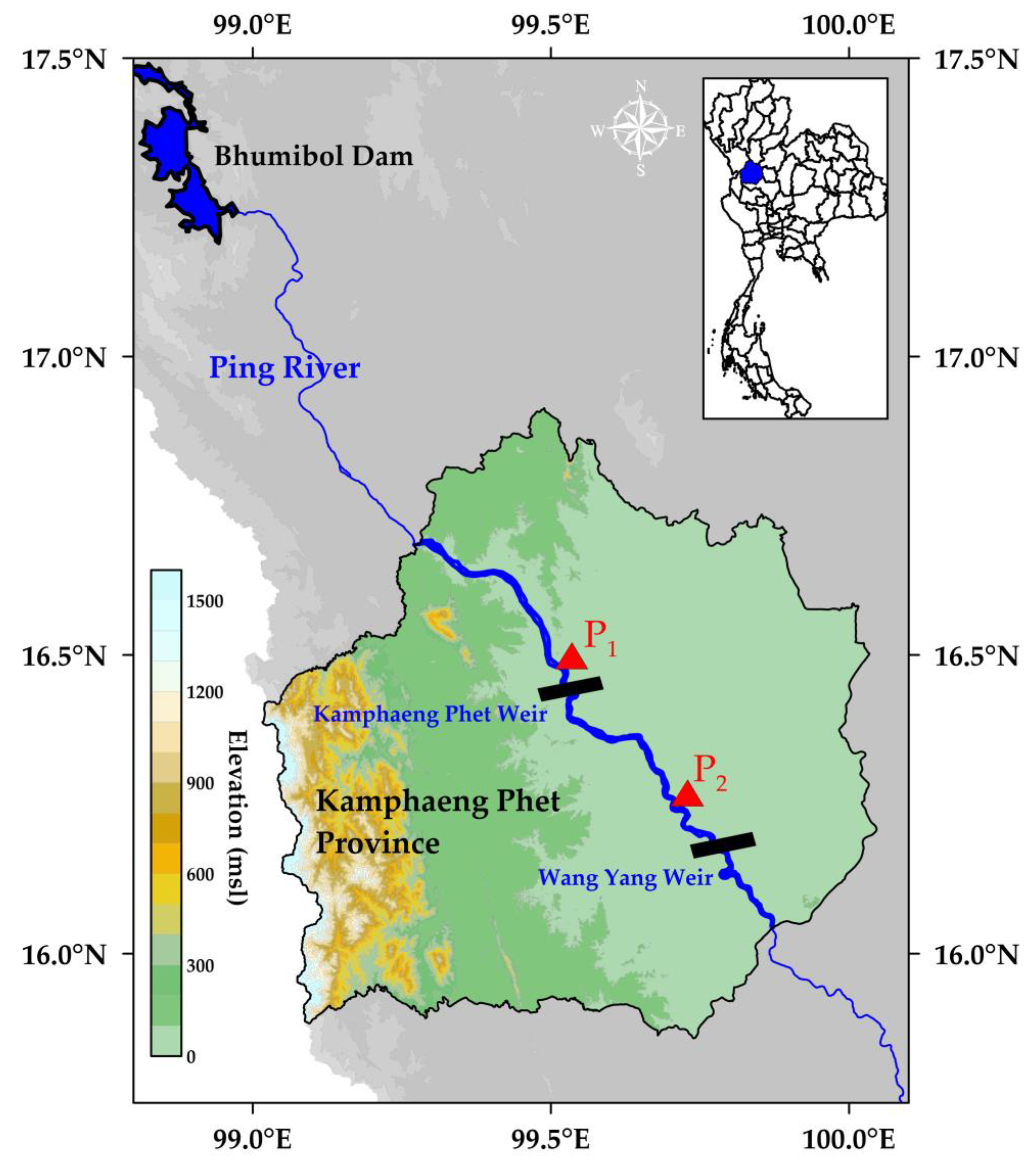
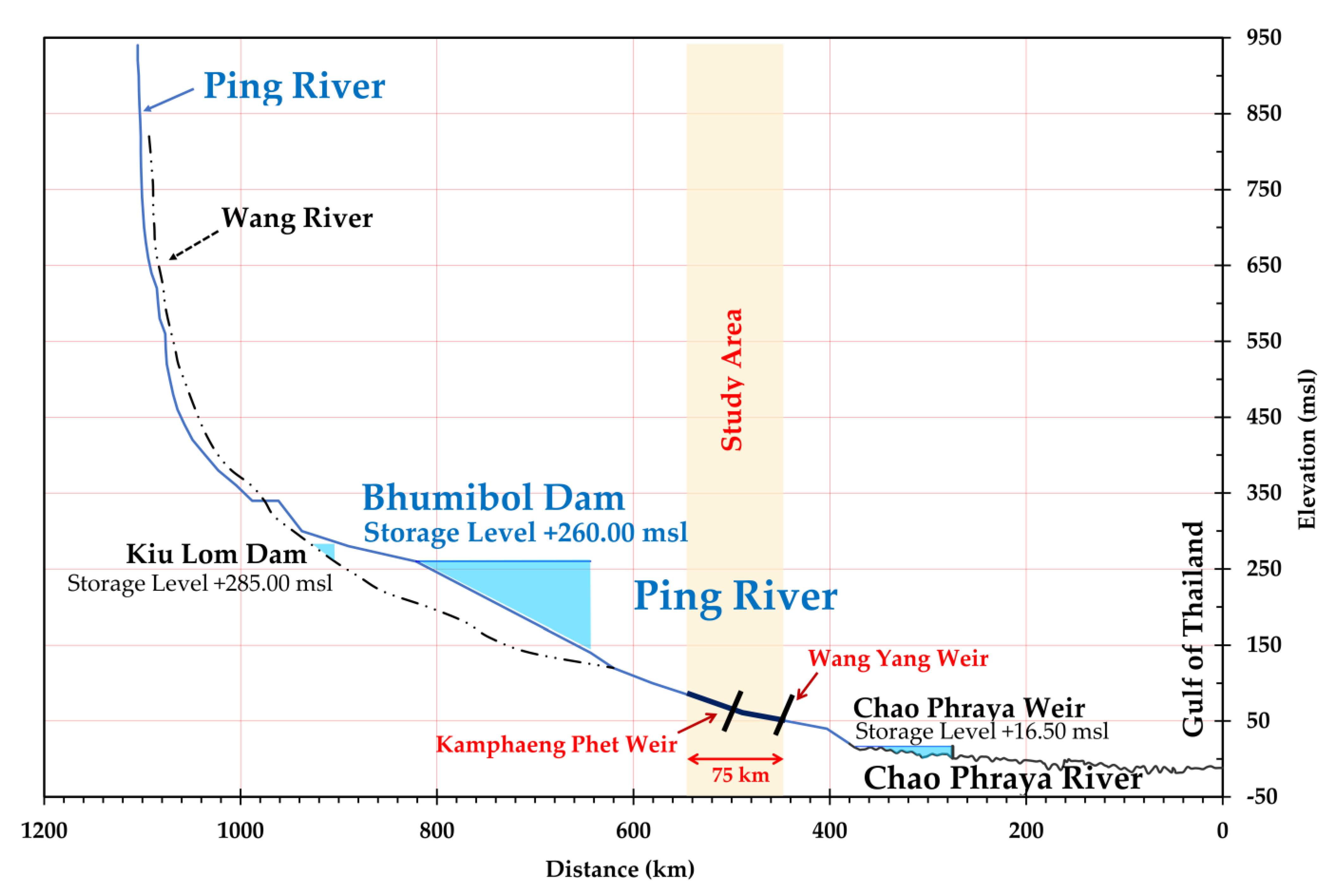
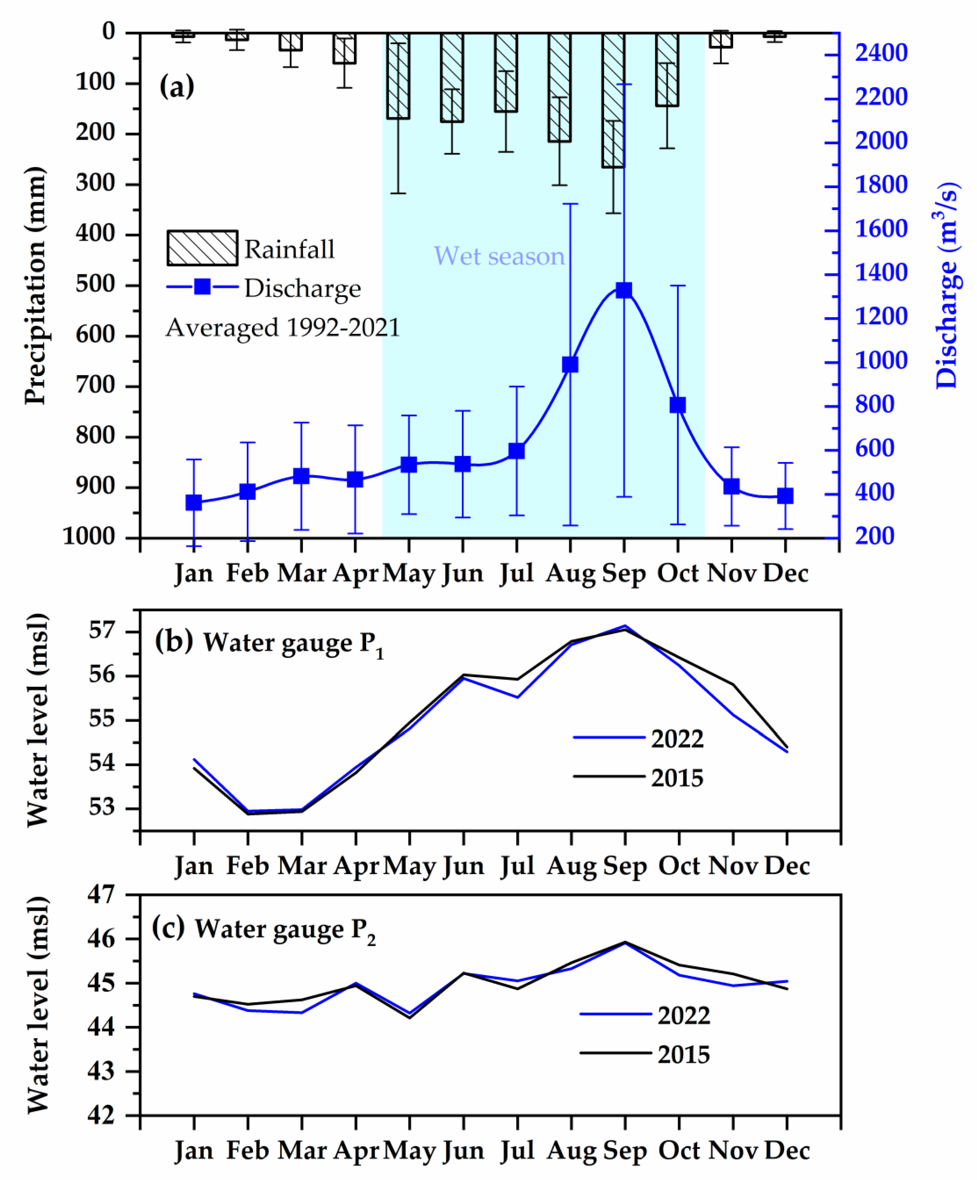
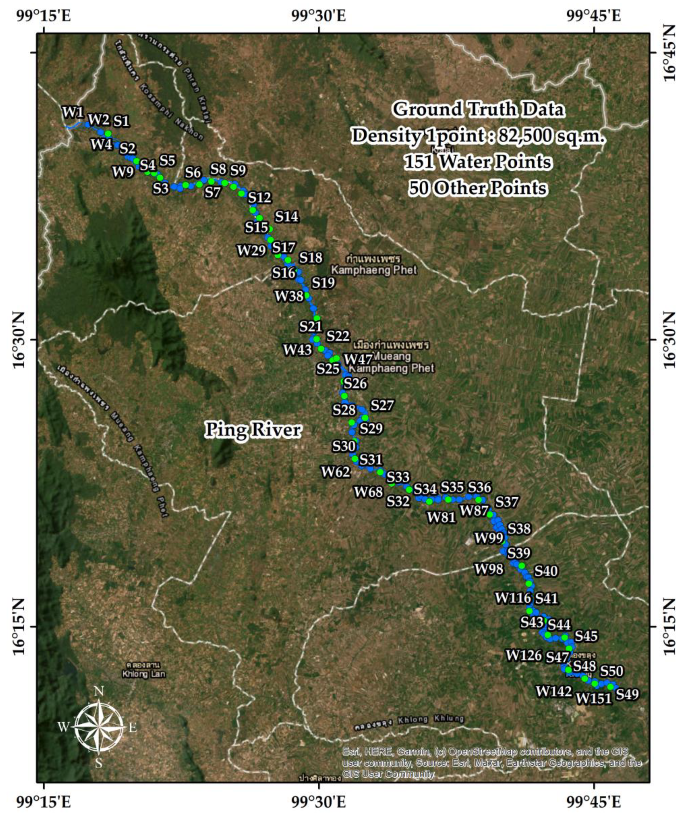
2.1. Study Area

The present study focuses on the Ping River in Kamphaeng Phet Province, as depicted in Figure 1. The Ping River Basin is one of eight sub-basins within the Chao Phraya Basin. The Ping River is a major upstream tributary that flows southward and eventually joins the Chao Phraya River at the central low-lying plain before emptying into the Gulf of Thailand. The Ping River Basin spans 44,688 km2, accounting for approximately 22% of the Chao Phraya River Basin and contributing 24% (6.97 × 10⁹ m3) of the total average annual runoff [17]. Terraced mountains characterize the topography of the Ping River Basin, with 55.5% of the basin’s area lying in the elevation range of 500–1000 m (Figure 2).
The climate in the area is mainly influenced by the southwest and northeast monsoons, as well as depression from the South China Sea during July and September, resulting in heavy rainfall from May to October. The average annual precipitation is 1117 mm, with an average yearly temperature of 26.7 °C. Nearly 88% (984 mm) of rainfall occurs during the rainy season (May–October), as shown in Figure 3a. The main channel of the Ping River is 658 km long, but the study area spans approximately 75 km in river length to fit within one satellite image. The river runoff flows from north to south, and the stream flow is seasonal, with wet and dry seasons. September has the highest discharge, averaging 1328 m3/s, while the lowest discharge occurs from January to March, averaging less than 361 m3/s (Figure 3a). River water levels also respond to the discharge variation and monsoon precipitation (Figure 3b,c). Climate change and variability can significantly impact the basin’s water resources, as evidenced by trends in climate indices such as a decrease in precipitation and an increase in temperature indices [4,24]. Furthermore, the basin is prone to environmental issues related to river flow during the wet and dry seasons, including flooding during the wet season and drought during the dry season. Hence, two rockfill weirs are Kamphaeng Phet weir and Wang Yang weir, which regulate water flow and reduce flooding (Figure 1).
The geological setting of the Ping riverbank is known for its extensive braiding patterns. It is characterized by multiple shallow channels that split and rejoin around mid-channel bars and islands and are comprised of sedimentary rocks, such as sandstone and shale, which are susceptible to erosion and instability [25]. The river’s flow and geological conditions have created a dynamic and constantly changing landscape. Additionally, the presence of faults and joints in the rocks, as well as variations in rock permeability and strength, can contribute to instability along the riverbank.

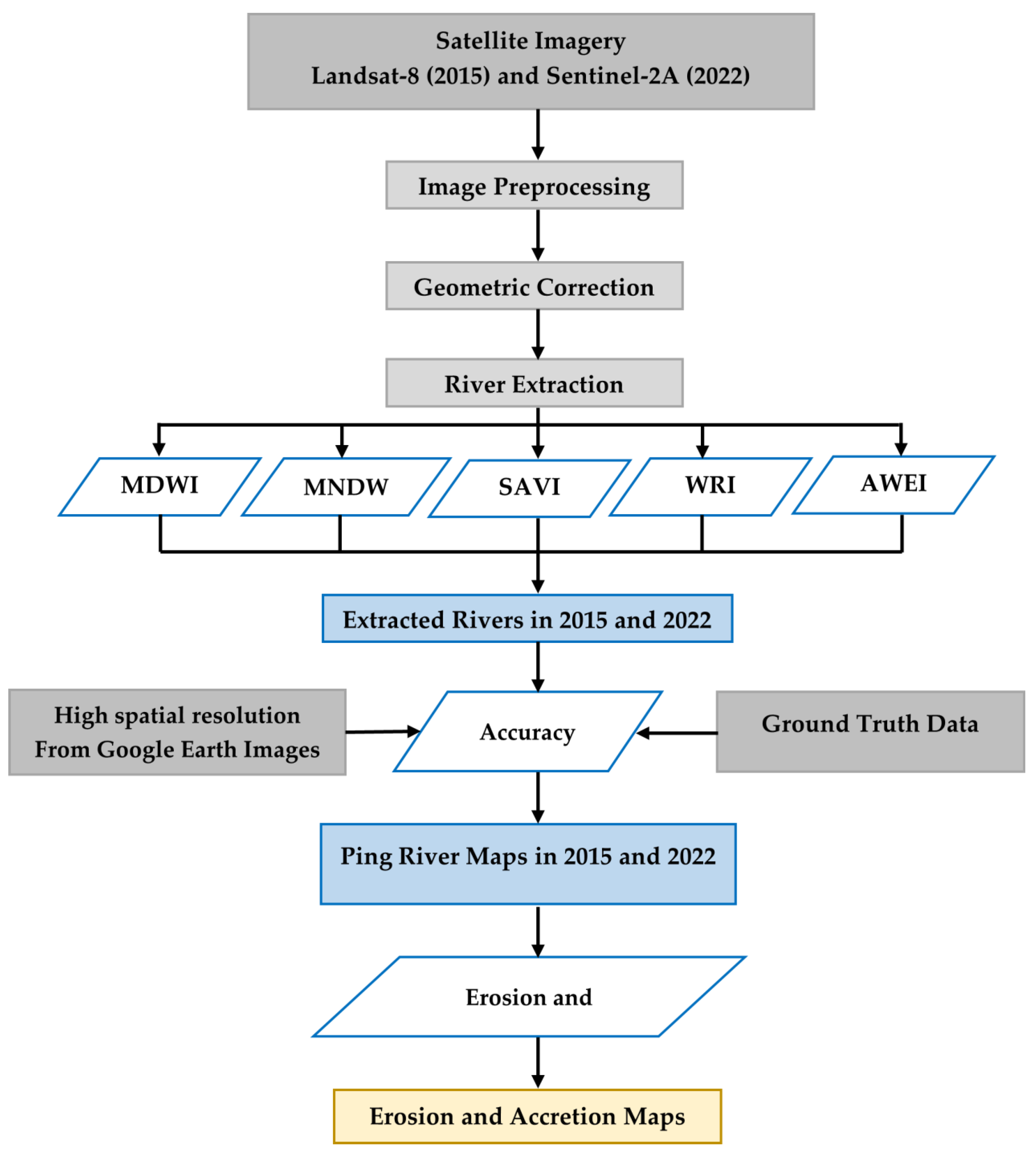
2.2. Satellite Imagery

This study obtained satellite imagery from Landsat-8 and Sentinel-2A sources (Table 1). The imaging period was from June 2015 to June 2022. For comparison with Landsat-8, there were six cloud-free dates across 35 different scenes for the wet season of 2015. Meanwhile, compared with Sentinel-2A, there were five dates across 54 scenes. The average number of dates per scene was 4 for Landsat-8 and 5 for Sentinel-2A. Images from the same month were selected to minimize seasonal variations in water level and surface water area.
Landsat-8, owned and operated by NASA and the USGS, provides globally georeferenced images and image processing capabilities. Its instruments, the Operational Land Imager and the Thermal Infrared Sensor, support various applications, such as cartography, land use, forestry management, coastal zone monitoring, and flood risk management [26]. Landsat-8 was launched in 2013 and orbits the Earth at an altitude of 705 km with an inclination of 98 degrees [27]. It is equipped with optical imagery that can detect objects in the visible to the near-infrared range with a resolution of 30 m and a width of 185 km. Therefore, Landsat-8 products in 2015 are suitable for studying the river as the narrowest river width is about 35 m. However, two water pixels might be mixed with other land cover. The reported overall accuracy of classified Landsat-8 was 75.6% for classifying bare land, forest, settlement, vegetation, and water [28]. The differences in water level (mean absolute 13.9 cm (0.25%) for station P1 and 12.3 cm (0.16%) for station P2, Figure 3b,c) and the uncertainty of the spectral detections of the satellite might affect the range of water in the riverbed and the accuracy of obtained erosion and deposition areas.
Sentinel-2A is a European optical imaging satellite that was launched in 2015 as part of the Copernicus Program of the ESA. It orbits the Earth at an altitude of 786 km. Sentinel-2A has a high-resolution multispectral imager with a resolution of 10–60 m and 13 spectral bands [29] that support global terrestrial observations for applications such as forest monitoring, land cover change detection, and natural disaster management.
The data used in this study were acquired from the official websites of Landsat-8 and Sentinel-2A as level L1T and L1C data, respectively. Only the data processed with the ESA’s version 02.04 system since 2017 were used for Sentinel-2A, following the ESA’s recommendations, due to errors in the previous processing software. The overall accuracy for classified Sentinel-2A was 100% for the water class [28]. The cloud and cloud shadow masking were carried out using the Fmask 4.0 algorithm [30]. Dates with less than 10% cloud covers were selected through this process to minimize the impact of undetected clouds and cloud shadows and achieve the most accurate results. However, in the fluvial processes, such low-resolution satellite imagery might reduce the accuracy of the research results and is only allowed for estimation.

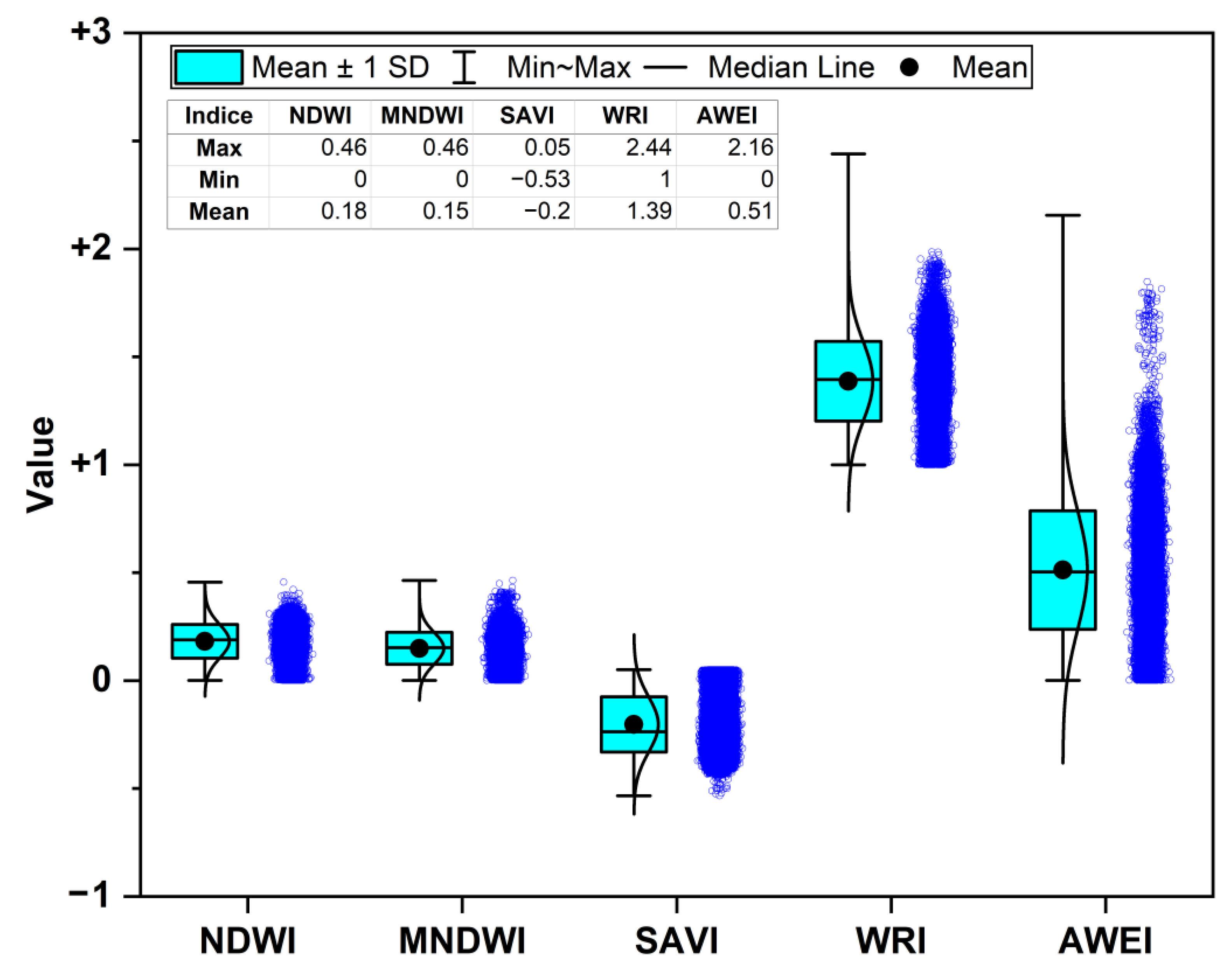
2.3. Satellite Image Extraction Method

This study devised a method to extract the Ping River from satellite images, as illustrated in Figure 4. The satellite data were acquired from online archives and underwent preprocessing, including atmospheric correction, geometric correction, and image mosaic. The images were then re-sampled to a 15 m spatial resolution using the average resampling method in the GDAL program (version 3.5.1) [31].
To analyze the satellite images, five different techniques were employed to extract streams, including the Normalized Difference Water Index (NDWI), Modified Normalized Difference Water Index (MNDWI), Soil-Adjusted Vegetation Index (SAVI), Water Ratio Index (WRI), and Automated Water Extraction Index (AWEI). During the surface water extraction process, a threshold of 0 was used for each index map. However, previous studies have indicated that a threshold of 0 might not always result in the best extraction performance in all areas [32,33,34]. Therefore, an optimum threshold was determined based on the Otsu threshold method [35] to achieve the highest overall accuracy. Additionally, indices with better extraction abilities may be combined to enhance the separability between water and non-water surfaces, as determined by evaluation matrices.
Ground truth locations surveyed in 2022 were used for validation purposes. However, no ground survey data were available for 2015, so the Google Earth product was utilized instead. A total of 201 locations were selected, including 151 water locations and 50 other types, with a density of 1 site per 82,500 square kilometers (Figure 5). An overlay technique was used each year to determine representative river lines. Erosion and deposition areas were computed by considering the river in 2015 and 2022 and unchanged areas. The riverbank erosion area was defined as the difference between the river area in 2022 and the unchanged river area between 2015 and 2022, while the channel deposition was examined by the difference of river shape in 2015 and the unchanged area. The left and right riverbank were divided by thalweg, and each bank’s erosion and deposition were also estimated.

2.3.1. Normalized Difference Water Index (NDWI)

The Normalized Difference Water Index (NDWI) is a technique utilized in satellite imagery analysis to distinguish open water features by utilizing the near-infrared (NIR) and visible green (GREEN) spectral bands [36]. The calculation of NDWI is performed using the following formula:
NDWI = (GREEN − NIR)/(GREEN + NIR)
The Normalized Difference Water Index is considered an effective index for differentiating land and water due to the high absorption of electromagnetic radiation by water surfaces, resulting in low radiation reflectance. However, it can lead to errors in estimating construction sites as water bodies. Hence, it is important to consider the ratio of NIR and GREEN wavelengths. The Normalized Difference Water Index ranges from −1 to 1, with 1 indicating water bodies or high humidity and −1 indicating dry areas or a lack of moisture [37]. The calculation of NDWI for this study was performed using the raster calculator toolbox in the ArcMap program. Normalized Difference Water Index values ranging from 0.004 to 0.46 (with an average of 0.18) were considered as water bodies (Figure 6).

2.3.2. Modified Normalized Difference Water Index (MNDWI)

The Modified Normalized Difference Water Index (MNDWI) effectively differentiates between water and urban areas in satellite images. This method utilizes the visible green (GREEN) and short-wave infrared 1 (SWIR1) spectral bands [32]. The MNDWI range (0.004–0.46, with an average of 0.15) for the waterbody was equal to that of NDWI (Figure 6).
MNDWI = (GREEN − SWIR1)/(GREEN + SWIR1)

2.3.3. Soil Adjustment Vegetation Index (SAVI)

The Normalized Difference Water Index products derived are inherently unstable, varying with soil color, soil moisture, and saturation effects caused by dense vegetation [38]. The Soil-Adjusted Vegetation Index (SAVI) is designed to correct for the instability of NDWI products. The Soil-Adjusted Vegetation Index reduces the impact of soil brightness by using red (RED) and near-infrared (NIR) wavelengths [39]. The SAVI index is given as follows:
SAVI = ((NIR − RED)/(NIR + RED + L)) × (1 + L)
where L is a factor to adjust the canopy background; a value of 0.5 was found to minimize soil brightness variations and eliminate the need for additional calibration for different soils [40]. It was found that the transformation virtually eliminates soil-induced variations in vegetation indices. The study extracts satellite imagery data with SAVI using the red and near-infrared bands via a raster calculator in the ArcMap program. The SAVI values ranged from −0.53 to 0.05 for the waterbody (Figure 6).

2.3.4. Water Ratio Index (WRI)

The Water Ratio Index (WRI) is a method that considers the dominant spectral reflectance of water. It is calculated as the ratio between the reflectance of visible green (GREEN) and red (RED) spectral bands to the total reflectance of near-infrared and short-wave infrared 1 (SWIR1) bands. The value of the WRI for waterbodies is greater than 1. The WRI value of the waterbody is greater than 1 [41,42], where WRI is defined as:
WRI = (GREEN + RED)/(NIR + SWIR1)

2.3.5. Automated Water Extraction Index (AWEI)

The Automated Water Extraction Index (AWEI) aims to enhance land cover classification accuracy into binary water and non-water under various environmental conditions. This is achieved by utilizing multiple spectral bands (blue, green, NIR, SWIR1, and SWIR2) and stabilizing the threshold of 0 used to distinguish water and non-water pixels by forcing non-water pixels below 0 and water pixels above 0 [33]. The subscript “sh” in the equation is introduced to effectively eliminate non-watery pixels, including dark-built surfaces in urban areas, resulting in improved accuracy by removing shadow pixels.
AWEIsh = BLUE + 2.5 × GREEN − 1.5 × (NIR + SWIR1) − 0.25 × SWIR2

2.4. Model Validation

A confusion matrix is a tool that summarizes the results of image classification predictions. It provides a count of correct and incorrect predictions, broken down by class. The observed category set is compared to the predicted classification set. There are four possible outcomes for each column [43,44], as described in Table 2. These are: (1) the classifier correctly identifies a water sample, referred to as a true positive (TP), (2) the classifier incorrectly categorizes a water sample as land or vegetation, resulting in a false-negative (FN), (3) the classifier misclassifies a land sample as water, referred to as a false-positive (FP), and (4) the classifier correctly identifies a land sample as a true negative (TN).
The accuracy of the river line data extracted from satellite imagery was validated by comparing it to the riverbanks from the Google Earth base map and ground survey data (Figure 5). The comparison results were used to create a confusion matrix, which summarizes the prediction results of the image classification. The accuracy, precision, and sensitivity values were calculated based on the information contained in the confusion matrix.
Accuracy = (TP + TN)/(TP + TN + FP + FN)
Precision = TP/(TP + FP)
Sensitivity = TP/(TP + FN)

3. Results and Discussion

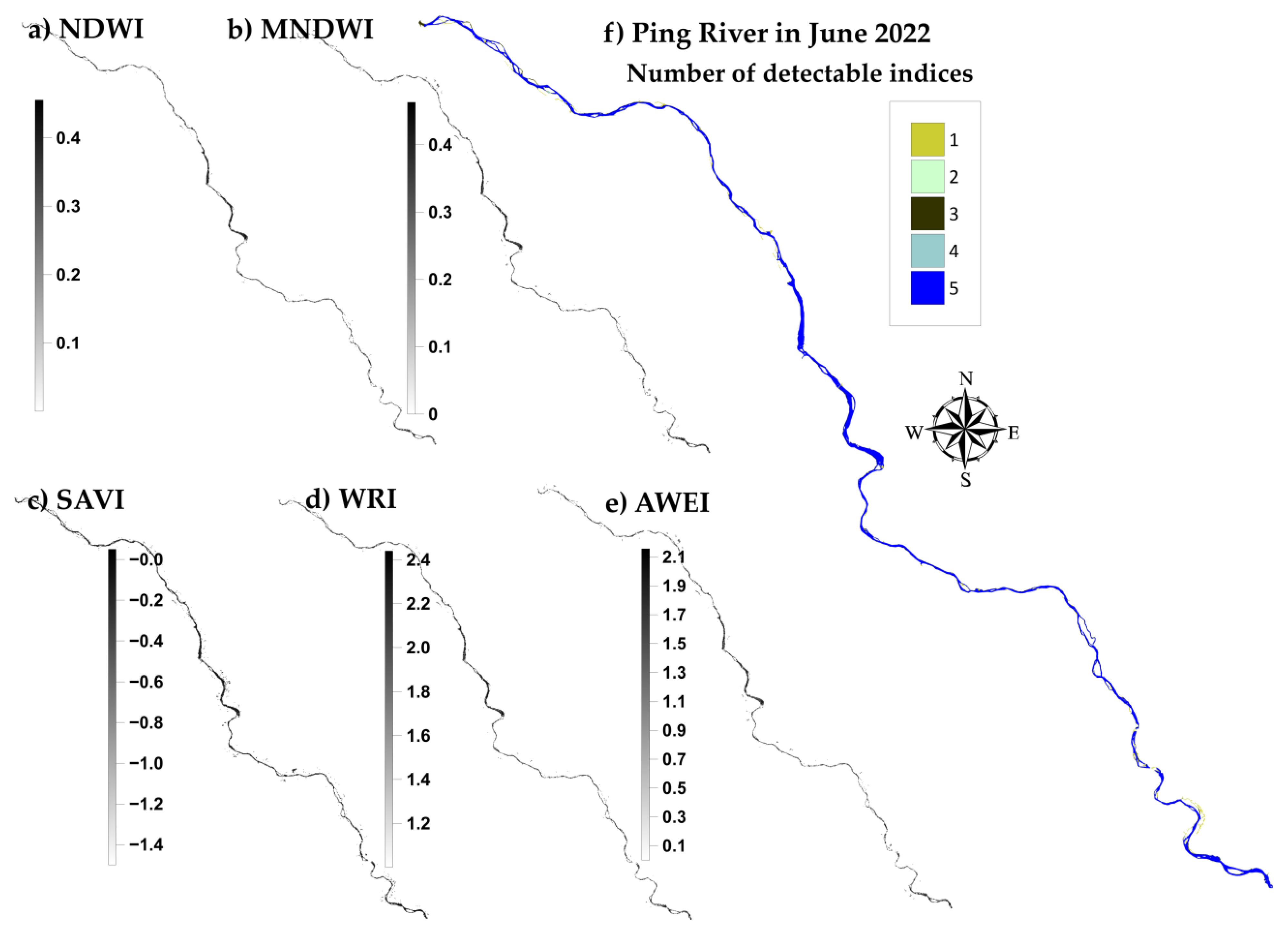
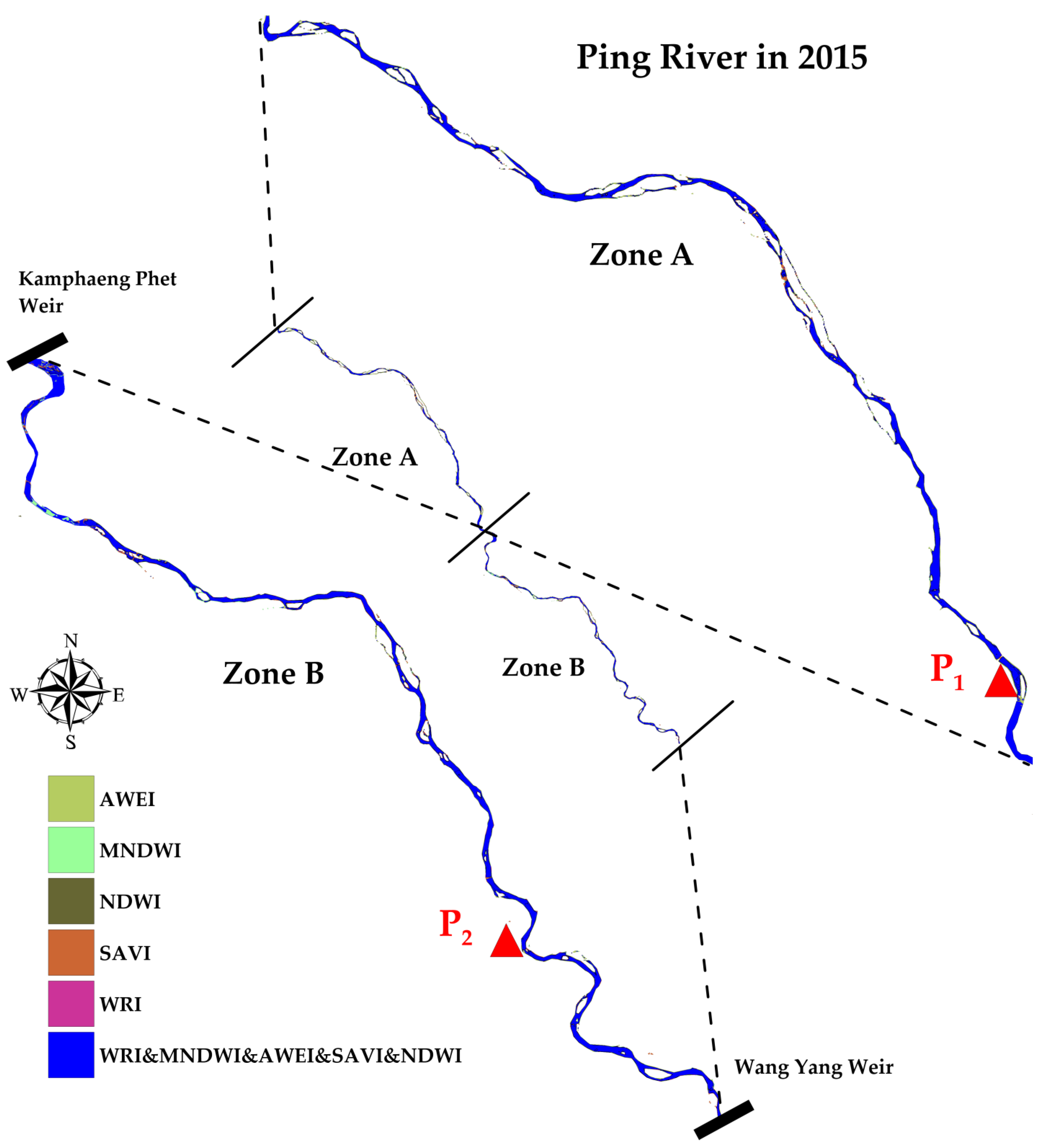
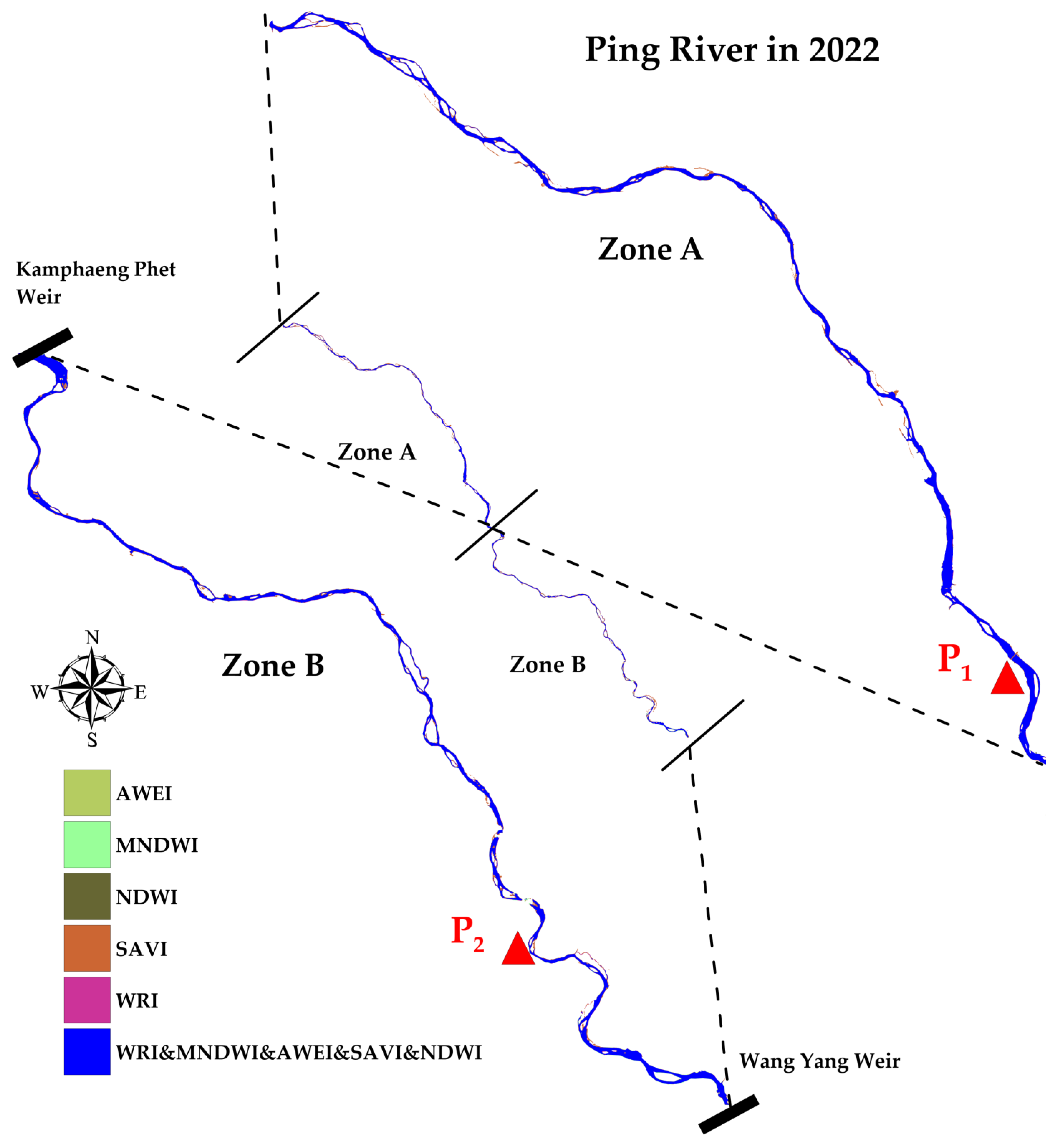
3.1. Ping Rivershape Extracted from Satellite Images

The watercourse extraction was performed using five index methods, as determined by the threshold values illustrated in Figure 6. Figure 7 presents the resultant map of the Ping River in 2015, derived from a Landsat-8 image using the five indices, along with a box plot of the pixel value distribution (Figure 6). The extracted streams using these five index methods are not significantly dissimilar. All indices are capable of detecting the Ping River water along the thalweg or its deepest channel (Figure 7f). The zero-threshold value used for the AWEI index demonstrates the ability to effectively separate the water (Figure 7e). Similarly, other indices perform well in separating the river, with some errors in water hyacinth, shadow, and narrow areas. The weakest performance was demonstrated by the NDWI, which requires additional effort to separate the waterbodies from shadows and dense forests (Figure 7a).
Furthermore, the SAVI is particularly useful in distinguishing vegetation from water, and it is able to account for variations in soil brightness. This makes it a good choice for detecting braided rivers where vegetation may be present (Figure 7c). However, the SAVI may be less effective in areas with very sparse vegetation or with mixed pixel types.
On the other hand, the WRI is designed specifically to differentiate between water and other types of land cover. It is particularly sensitive to water features, making it a good choice for extracting braided river features from Landsat-8 imagery (Figure 7d). However, the WRI may not perform as well in areas where there are other types of water bodies (e.g., lakes or wetlands) present.
The extracted map of the Ping River in 2022 using the five water indices is shown in Figure 8, which was derived from a Sentinel-2A image. The streams extracted through these five methods were similar. The high-resolution image provided by Sentinel-2A improved the accuracy and completeness of the extracted river compared to the Landsat-8 image.
The four water-related indices (NDWI, MNDWI, WRI, and AWEI) effectively reflected water bodies based on their values. [45]. The Normalized Difference Water Index and MNDWI are both helpful in detecting water bodies in general. However, they might not be ideal for specifically identifying braided rivers as they do not consider the distinct spectral characteristics of braided rivers (Figure 8a,b). The SAVI index effectively detects water hyacinths and accurately represents the river shape, including waterbodies and ponds along the riverside. This is because the water hyacinth has higher NIR reflectance values than other associated plant species [46,47], as shown in Figure 8c. The AWEI might not be effective in identifying braided rivers from Sentinel-2A imagery specifically because it was primarily designed to detect water from vegetation, not sand (Figure 8e). Among the indices, the WRI appeared to be a more reliable indicator, as it was the only index of the five that enhanced water surfaces (Figure 8d). The WRI has shown promise in detecting braided rivers from Sentinel-2A imagery. It considers the unique spectral signature of braided rivers, which includes both high reflectance in the green and red bands and low reflectance in the blue band.

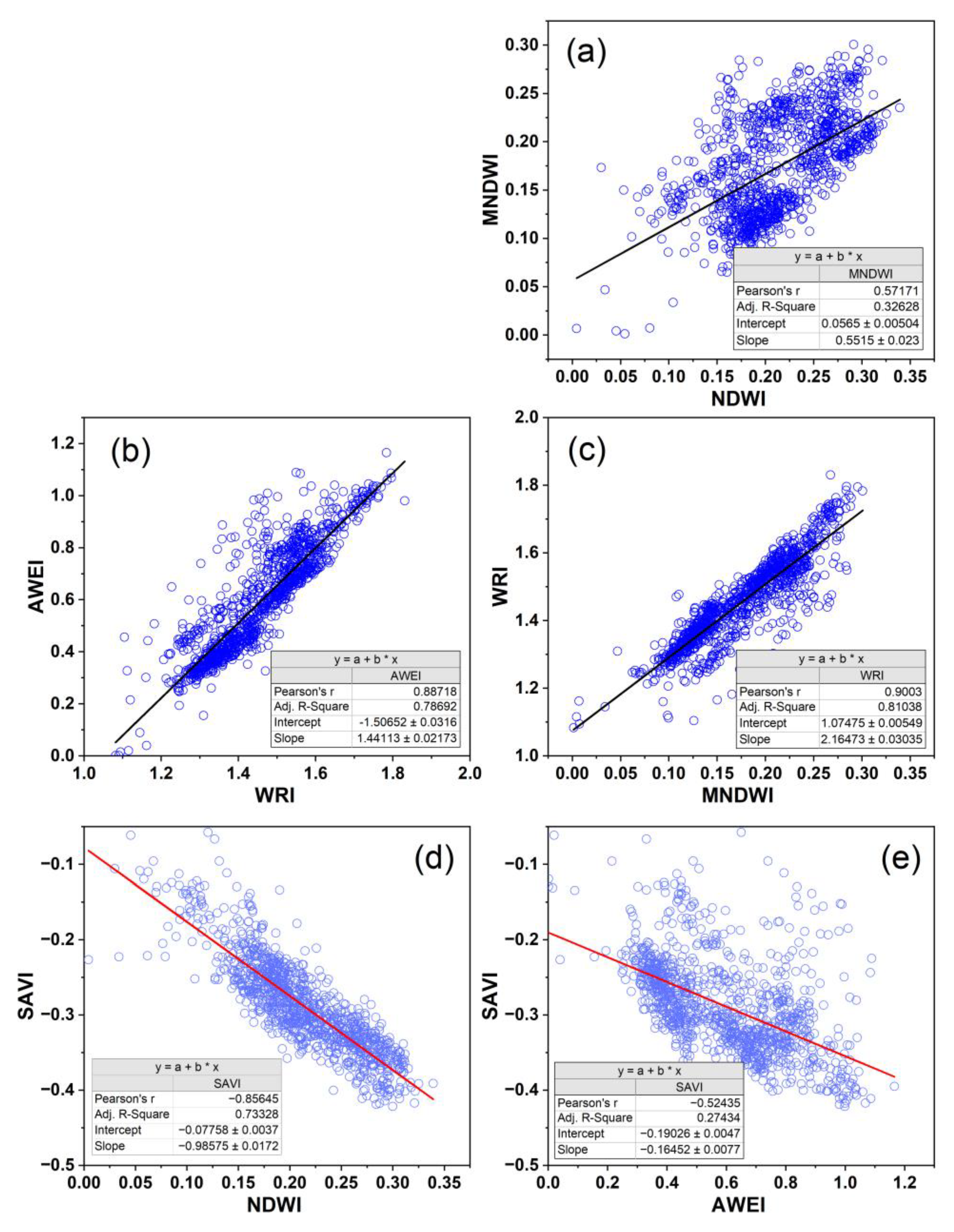
3.2. Result Consistency and Accuracy

In order to evaluate the relationships between different variables, the NDWI, MNDWI, NDMI, WRI, and AWEI reflectance index values were plotted in scatter plots (Figure 9). The coefficient of determination (R2) was used to assess the effectiveness of the regression model in explaining the variability of the data. High R2 values close to 1 indicate a good fit for the model [48].
The study found strong correlations between the five water indices at a 95% confidence level (p < 0.05, n = 65,351, Figure 9). Positive values represent surface water (Figure 7 and Figure 8), and four of the index methods (NDWI, MNDWI, WRI, AWEI) had positive correlations with each other (Figure 9a–c). The SAVI showed a significant negative relationship between the NDWI and the AWEI, with negative values indicating waterbodies in the study area (Figure 7c and Figure 8c). However, some regions observed weak correlations due to the narrow range of index values for water-land cover classes [45].
Two sets of ground truth data were used for validation, including high-resolution images from Google Earth in 2015 (201 stations, Figure 5) and a ground survey in June 2022 at the same locations (201 stations, Figure 5). The data were further divided into two categories, 151 stations along the mid-line of a stream and 50 stations located 30 m away from the nearest riverbank. This second category was equivalent to two pixels of the re-sampled image due to minimizing pixels being a mixture of water, vegetation, and soil. To assess the results, a confusion matrix was used to compare the extraction results from each method with the Google Earth samples from 2015 and the ground survey from 2022, including accuracy, precision, and sensitivity (Table 3 and Table 4).
The stream in 2015 (2022) obtained from the NDWI extraction was 79 (93) percent accurate and 100 (97) percent precise. The NDWI measures presented water in pixels. Shadows, saturated soil, and plants are also detected. False positives can occur when non-water features are identified as water (Table 3 and Table 4). The MNDWI results provide 89 (90) percent accuracy and 99 (96) percent precision for 2015 (2022). The MNDWI reduces vegetation effects better than the NDWI. However, the MNDWI detects shadows and moist soil, resulting in false positives (Table 3 and Table 4). The river in 2015 (2022) obtained through the SAVI extraction was 86 (95) percent accurate and 98 (96) percent precise. The SAVI is commonly used to assess vegetation density. The SAVI can also misidentify shadows and soil as water bodies. The WRI results provide 83 (95) percent accuracy and 99 (98) percent precision for 2015 (2022). The WRI is an index that is used to identify surface water features. However, it probably detects other features, such as shadows, wet soil, and vegetation, leading to false positives. The AWEI is designed to improve the detection of water bodies by reducing the effects of soil and vegetation. As a result, the AWEI extraction of streams was the most accurate for Landsat-8 in 2015, with 90 percent accuracy and 99 percent precision. However, the AWEI results were less accurate in 2022 (Table 4) compared to 2015 (Table 3). It might detect other features, such as shadows from the Sentinel-2A images, leading to false positives.
The SAVI and WRI were the most effective methods for the 2022 environment, based on NIR (785–900 nm for Sentinel-2A, 850–880 nm for Landsat-8). The SAVI (≤−0.53) and WRI (≥1) values were interpreted as water areas due to the high concentration of chlorophyll-a in the water hyacinth [49], which is sensitive to the NIR spectrum due to the high reflectance of its internal leaf structure [47].
Regarding satellite imagery comparison, there are variations in the sensor responses and spectral properties of target pixels between Sentinel-2A and Landsat-8 [27,50]. Sentinel-2A offers imagery with a higher level of detail. The outcomes from Sentinel-2A were more precise than those from Landsat-8 (as seen in Table 4). Despite the higher resolution, Sentinel-2A has some bands with spectral characteristics similar to those of the prominent bands of Landsat-8. The reflectance values from Sentinel-2A are more closely aligned with those from Landsat-8 [51,52]. Therefore, for this study, the threshold of each water index derived from Landsat-8 was applied to Sentinel-2A.
Previously established water indices (such as NDWI or MNDWI) utilized green and NIR or SWIR bands to distinguish water bodies from non-water features, as water and non-water features exhibit significant differences in these three bands. However, the results of experiments showed that relying solely on the NIR band in a water index may lead to the loss of some water features (e.g., murky water, small waterbodies), while relying solely on the SWIR band can result in the misclassification of some land features such as shaded pixels as water. Hence, the index based on both NIR and SWIR, such as the AWEI and WRI (as described in Equations (4) and (5)), was found to classify water accurately, as demonstrated in Table 3 and Figure 10 and Figure 11.
These figures indicate that most indices can effectively distinguish water from other land features. Some indices, such as the NDWI for Landsat-8 (Figure 10) and the MNDWI for Sentinel-2A (Figure 11), showed a loss of small water bodies where the main channel was divided by aits or eyots, riverine islands formed by sediment deposition or emerging river bars at low water levels. To minimize these errors, it is recommended to use multiple indices and the visual interpretation of satellite images to confirm the presence of the braided river (Figure 10 and Figure 11). Additionally, pre-processing steps such as image calibration, atmospheric correction, and geometric correction can be applied to satellite images to reduce errors.

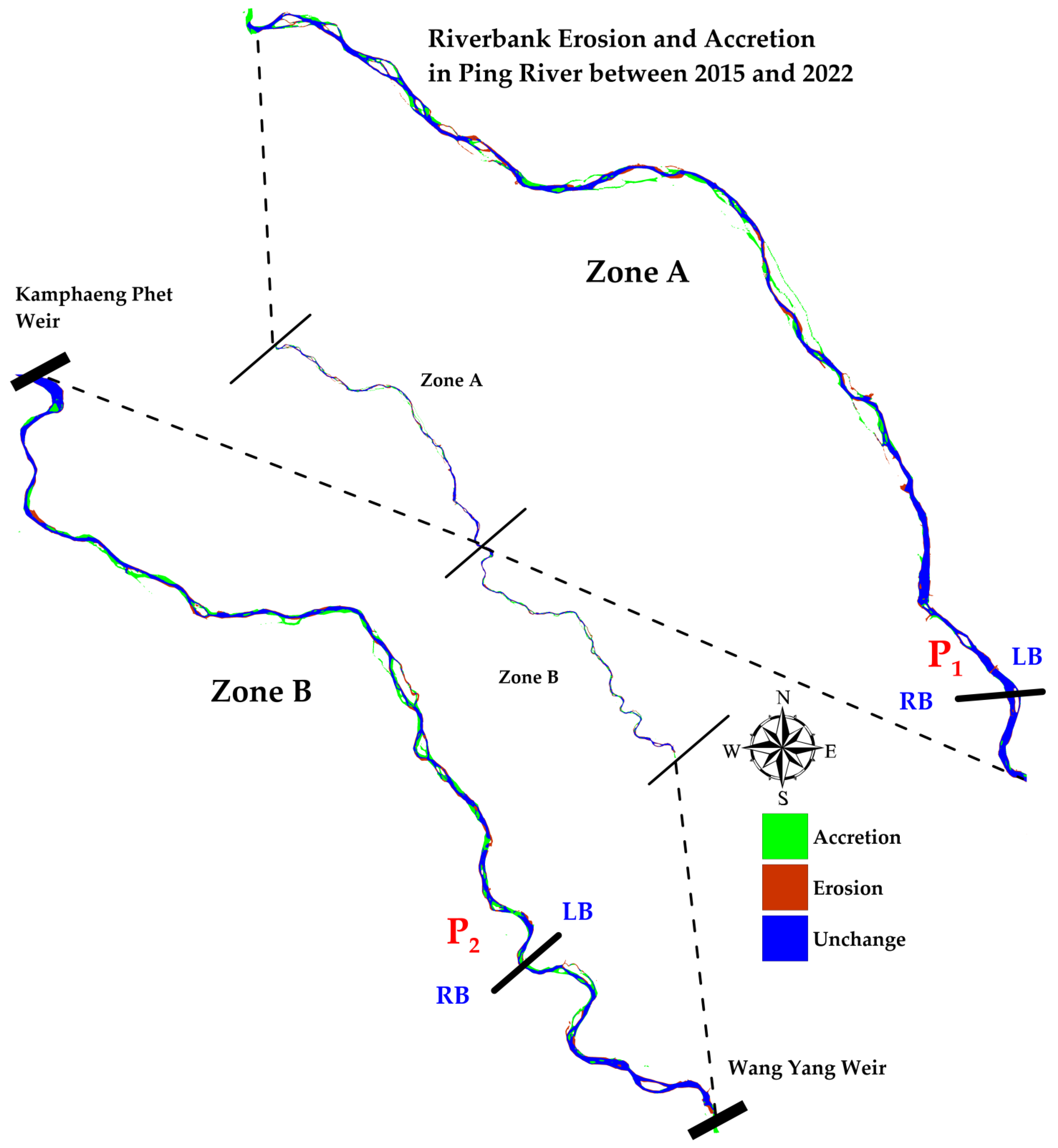
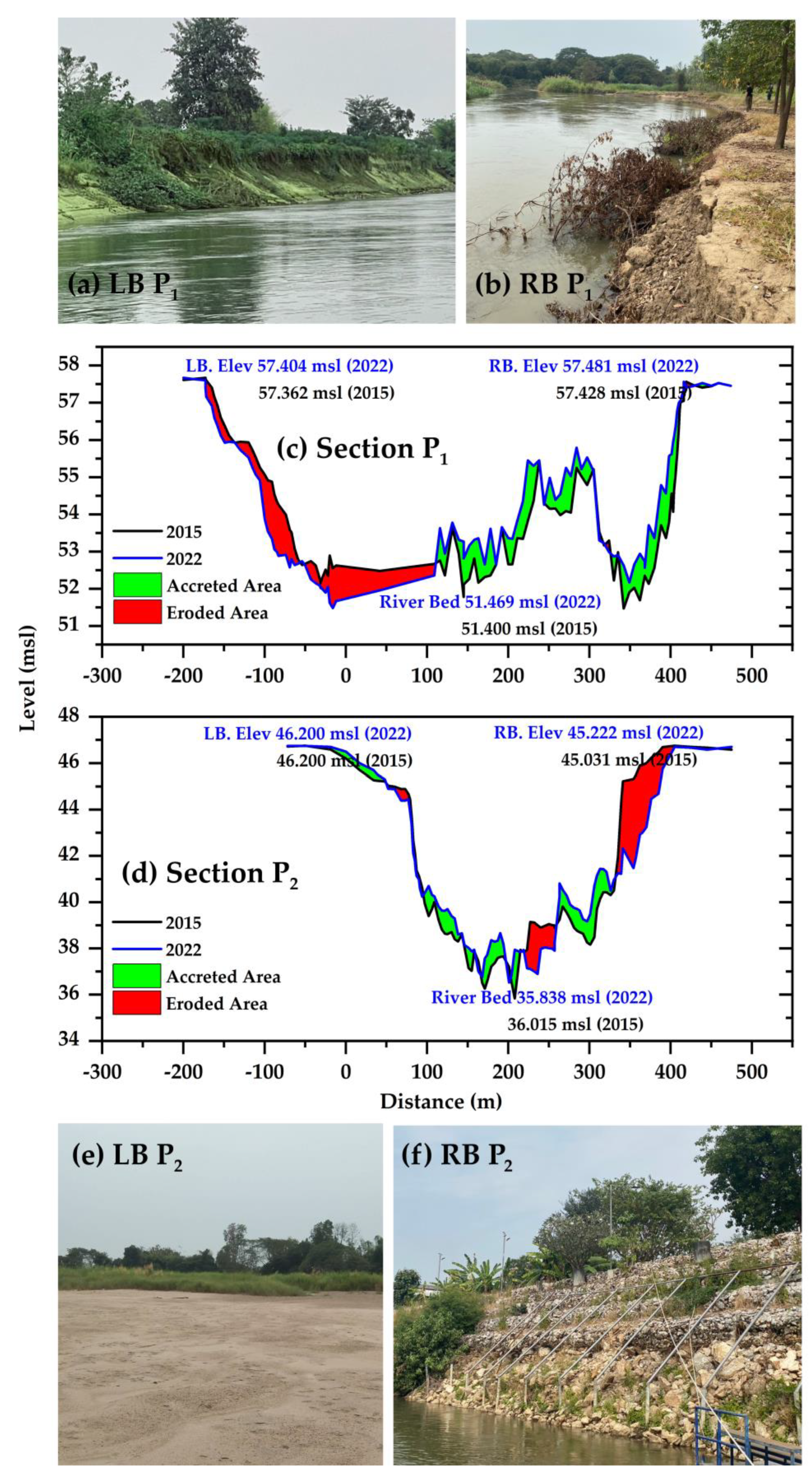
3.3. Riverbank Erosion and Deposition

The Ping River flows from south to north, and two weirs exist in the studied section, Figure 1. This river exhibits fluvial processes of erosion and deposition (Figure 12 and Figure 13), characteristic of braided river systems [13]. Braided rivers are characterized by multiple interconnected channels separated by bars of sediment. The channels typically have shallow depths and a high width-to-depth ratio, and they tend to shift and migrate over time due to variations in water flow and sediment deposition [53]. The area between the midstream and downstream is flat, causing the riverbank to erode and deposit sediment on the convex bank. The depositional bank is formed by the accumulation of coarse sand and gravel, alternating with ridges and swales, known as sand shoals, that divide the main channel of the Ping River into smaller waterways (Figure 12).
Erosion occurs when the force of the river’s flow removes sediment from the riverbed and banks, widening and deepening the river channels (Figure 13). This erosion is typically caused by the high velocity and turbulent flow of water, which is common in braided river systems [54]. The erosion in the Ping River leads to the formation of sandbars and islands within the river channels. Deposition, on the other hand, occurs when sediment carried by the river’s flow settles and accumulates in the riverbed and banks. This deposition can occur when the river’s flow slows down, such as when it enters wider channels or when there is a decrease in the slope of the river [55], as seen in zone B in Figure 12. The deposition in the Ping River leads to the formation of bars of sediment (Figure 10, Figure 11, Figure 12 and Figure 13c), which can cause the river channels to split and braid, creating a network of streams referred to as a dendritic drainage pattern [56].
The dendritic drainage pattern of the Ping River refers to its branching network of tributaries, which resembles the structure of a tree. This type of drainage pattern is common in regions with uniform geology and slope [57]. In contrast to anastomosing rivers [58], which have multiple interconnected channels that are stable over time, braided rivers such as the Ping River tend to shift and change their channel patterns more frequently due to changes in water flow and sediment deposition.
The water map was generated by combining the results of five different indices using threshold values obtained from each index. Initially, a threshold value of 0 was used for all indices, resulting in a map highlighting dense shadows and deep river depths. The Otsu threshold method was then employed to separate water and the drainage network [35], using values such as 0.004 for the NDWI, −0.53 for the SAVI, and 1 for the WRI (Figure 6). This overlay technique was used to estimate the erosion and accretion area of the Ping River between 2015 and 2022 (Figure 12), with the stream data from the five indices (NDWI, MNDWI, SAVI, WRI, and AWEI) combined to represent the riverbank erosion and deposition more accurately. The average surface area of the Ping River decreased by 0.58 ± 0.44 km2 (Table 5), with the AWEI and SAVI results showing the most significant decrease in river area. The WRI results showed a minor decrease in the river area but were the most accurate, especially for Sentinel-2A in 2022 (Table 4). The river surface area was 16.88 km2 in 2015 and 16.51 km2 in 2022, with an estimated erosion area of 5.18 km2 and a deposition area of 5.55 km2 (Table 5). The erosion and accretion rates varied between the five methods, with an average erosion rate of 4.51 ± 0.67 km2 and an accretion rate of 5.09 ± 0.30 km2. The unchanged area for the overlaid data was 11.33 km2, with an average unchanged area of 10.35 ± 0.62 km2 across the five index results. The AWEI was able to integrate smaller waterbodies, resulting in higher erosion and accretion rates compared to the other methods.
However, there was an error range (5.47 to 20.90%) resulting from various factors, such as the error from water indices (Table 3 and Table 4) and spatial and spectral errors in satellites and different water levels (Figure 3b,c). The reported depositional area might include sediment accumulation and emerging river bars at the time of low water levels. The accuracy of detection from satellite images depends on several factors, including the type of object being detected, the quality of the satellite image, the radiometric calibration, and the atmospheric conditions during image acquisition. These factors contribute to the error range in the detection results. Consequently, to reduce the error, pre-processing steps such as image calibration, atmospheric correction, and geometric correction can be applied to satellite images. Additionally, image fusion techniques that combine images from multiple sensors or data sources and a period with a similar water level can improve detection accuracy.
The morphology of the Ping River has undergone significant alterations over seven years, as indicated by the presence of newly formed sandbars and the changes in the accretion and erosion of the riverbanks (Figure 13c,d). The study period reveals an increase in the sandbar and riverbank accretion areas, with a rate of 0.79 km2 per year, which is higher than the previous rate of 0.53 km2 per year between 2007 and 2017 [59]. Due to the non-cohesive nature of the Ping River and its floodplain system [60], high sedimentation is reflected in the swift growth of sandbars. However, this growth also causes instability in the river reaches as it alters the river flow direction and leads to increased flow velocity [59], putting the riverbank on the opposite side at risk (Figure 13a,b). Although the erosion occurred at both banks, the study found that riverbank erosion is predominantly found on the left bank (39.57 km length, Table 6) compared to the right bank (30.07 km length), indicating that the left bank of the Ping River has undergone more significant shifting compared to the right side. Hungry water is a phenomenon that occurs when the Kamphaeng Phet weir creates a turbulent flow of water that can erode the riverbed and banks downstream [61].
On the other hand, there was also the adverse effect of the Wang Yang weir downstream of the study boundary, which traps bed-load sediment and raises the riverbed upstream (Figure 12), particularly in areas with high bed-load sediment budget such as the Lower Ping River (Figure 13d). The increased sediment supply from the upstream mountain ranges and the presence of at least 30 sand and gravel mining businesses along the Ping River also contribute to the excessive sedimentation along the Ping River [62]. The combination of increased sediment supply and low water discharge leads to a significant decrease in the river’s depth and width (Figure 13e).
The gradient of the riverbed influences the velocity and direction of flow, which is a crucial aspect that shapes the river’s dynamics (Figure 2 and Figure 3). In some regions, the riverbank has become so steep and overhanging that it forms a cantilever-like structure (Figure 13b), which is vulnerable to collapse and failure [63]. In a cantilever riverbank failure, erosion initially occurs at the bank’s base or toe [20]. This erosion results in the soil or rock mass becoming increasingly unstable and leads to slumping and land sliding along the bank. As erosion continues, the bank becomes increasingly steep and overhanging, forming a cantilever-like structure supported only at its toe. A combination of natural and human factors has caused the occurrence of cantilever riverbank failure along the Ping River. This failure can result in various impacts, such as increased erosion and loss of crops and property. The river’s strong hydraulic forces and geological conditions are responsible for the instability and erosion of the riverbank [64]. The overuse of groundwater, deforestation, and development along the river also contribute to the problem [65].
Efforts are underway to address the issue of riverbank erosion along the Ping River. These include implementing stabilizing measures for the riverbank, such as building retaining walls, planting vegetation, and reinforcing the soil and rock materials at the bank’s toe (Figure 13f). Additionally, efforts are being made to manage water resources and minimize the impacts of deforestation and development along the river.

4. Conclusions

The study aimed to evaluate the performance of five water extraction indices. The results obtained from a default threshold of 0 indicated that the AWEI could reduce the omission errors in mapping water classes compared to the other indices using Landsat-8 images. The AWEI achieved the highest accuracy at 90% and precision at 99%. The WRI was also found to have satisfactory results compared to other water indices for Sentinel-2A products. The other indices may have produced less accurate results due to missing river sections, especially those with narrow channels. Furthermore, the Otsu threshold method was used to select the appropriate threshold for the NDWI, MNDWI, SAVI, and WRI. The SAVI also provided a more extensive water area in 2022 due to the response of the water hyacinth to Sentinel-2A reflectance, which was interpreted as the river area. These indices can be effective tools for identifying and extracting braided river features from Landsat-8 and Sentinel-2A images, but their effectiveness can depend on the specific characteristics of the landscape being analyzed.
The study also demonstrated that comparing the extracted rivers using the five water indices throughout 2015–2022 can reflect changes in river morphology. The study found that the river had undergone erosion of about 5.18 km2, mainly on the left riverbank, which was often attributed to the sand mining industry. Furthermore, the study observed that the Ping River had a growing sandbar along the river embankment and at the center of the river, increasing by 5.5 km2 from 2015 to 2022. The river had also changed direction, meandering back and forth over gently sloping terrain. Most of the deposited land was observed in the downstream terrain area of the Ping River. These study findings provide valuable insights into the river’s morphology and riverbank erosion/deposition, which could aid government organizations in creating sustainable river management policies and determining the best water indices for monitoring physical changes in tropical rivers.

Author Contributions

Conceptualization, J.L. and P.J.; methodology, J.L., T.S. and B.K.; software, T.S.; validation, J.L., P.J. and T.G.; formal analysis, T.S. and B.K.; investigation, P.J. and T.G.; resources, N.T. and T.S.; data curation, T.G. and J.L.; original manuscript writing, J.L. and P.C.; manuscript review and editing, P.J. and P.C.; visualization, T.S. and P.C.; supervision, P.J.; project administration, N.T.; funding acquisition, J.L. All authors have read and agreed to the published version of the manuscript.

Funding

This research was funded by Naresuan University, Grant Number: R2566C003.

Institutional Review Board Statement

Not applicable.

Informed Consent Statement

Not applicable.

Data Availability Statement

Not applicable.

Acknowledgments

The authors acknowledge the Department of Water Resources and the Royal Irrigation Department for supporting the hydrological data and the river cross-section. The authors also thank the Thailand Geo-Informatics and Space Technology Development Agency for providing satellite images and their technical support. This work was supported by Naresuan University [Grand Number R2566C003].

Conflicts of Interest

The authors declare no conflict of interest.

References

  1. Pörtner, H.O.; Roberts, D.C.; Adams, H.; Adler, C.; Aldunce, P.; Ali, E.; Begum, R.A.; Betts, R.; Kerr, R.B.; Biesbroek, R. Climate Change 2022: Impacts, Adaptation and Vulnerability; IPCC: Geneva, Switzerland, 2022.
  2. Laonamsai, J.; Ichiyanagi, K.; Kamdee, K.; Putthividhya, A.; Tanoue, M. Spatial and temporal distributions of stable isotopes in precipitation over Thailand. Hydrol. Process. 2021, 35, e13995. [Google Scholar] [CrossRef]
  3. Laonamsai, J.; Ichiyanagi, K.; Patsinghasanee, S.; Kamdee, K. Controls on Stable Isotopic Characteristics of Water Vapor over Thailand. Hydrol. Process. 2021, 35, e14202. [Google Scholar] [CrossRef]
  4. Laonamsai, J.; Ichiyanagi, K.; Patsinghasanee, S.; Kamdee, K.; Tomun, N. Application of Stable Isotopic Compositions of Rainfall Runoff for Evaporation Estimation in Thailand Mekong River Basin. Water 2022, 14, 2803. [Google Scholar] [CrossRef]
  5. Pavanelli, D.; Cavazza, C.; Lavrnić, S.; Toscano, A. The long-term effects of land use and climate changes on the hydro-morphology of the Reno river catchment (Northern Italy). Water 2019, 11, 1831. [Google Scholar] [CrossRef] [Green Version]
  6. Shrestha, S.; Imbulana, N.; Piman, T.; Chonwattana, S.; Ninsawat, S.; Babur, M. Multimodelling approach to the assessment of climate change impacts on hydrology and river morphology in the Chindwin River Basin, Myanmar. Catena 2020, 188, 104464. [Google Scholar] [CrossRef]
  7. Darby, S.E.; Leyland, J.; Kummu, M.; Räsänen, T.A.; Lauri, H. Decoding the drivers of bank erosion on the Mekong river: The roles of the Asian monsoon, tropical storms, and snowmelt. Water Resour. Res. 2013, 49, 2146–2163. [Google Scholar] [CrossRef]
  8. Alam, J.B.; Uddin, M.; Ahmed, J.U.; Cacovean, H.; Rahman, H.M.; Banik, B.K.; Yesmin, N. Study of morphological change of river old Brahmaputra and its social impacts by remote sensing. Geogr. Tech. 2007, 2, 1–11. [Google Scholar]
  9. Petts, G.E. Changing River Channels: The Geographical Tradition; Wiley: New York, NY, USA, 1995. [Google Scholar]
  10. Lewin, J.; Ashworth, P.J. Defining large river channel patterns: Alluvial exchange and plurality. Geomorphology 2014, 215, 83–98. [Google Scholar] [CrossRef]
  11. Leopold, L.B.; Wolman, M.G. River Channel Patterns: Braided, Meandering, and Straight; US Government Printing Office: Washington, DA, USA, 1957.
  12. Ahmed, A.A.; Fawzi, A. Meandering and bank erosion of the River Nile and its environmental impact on the area between Sohag and El-Minia, Egypt. Arab. J. Geosci. 2011, 4, 1–11. [Google Scholar] [CrossRef]
  13. Rust, B.R. Structure and process in a braided river. Sedimentology 1972, 18, 221–245. [Google Scholar] [CrossRef]
  14. Al-Bahrani, H.S. Spatial prediction and classification of water quality parameters for irrigation use in the Euphrates River (Iraq) using GIS and satellite image analyses. Int. J. Sustain. Dev. Plan. 2014, 9, 389–399. [Google Scholar] [CrossRef] [Green Version]
  15. Saprathet, T.; Losiri, C.; Sitthi, A.; Laonamsai, J. Monitoring of Morphological Change in Lam Phachi River Using Geo-informatics System. In Applied Geography and Geoinformatics for Sustainable Development: Proceedings of ICGGS 2022; Springer: Berlin/Heidelberg, Germany, 2022; pp. 51–64. [Google Scholar]
  16. Mukherjee, N.R.; Samuel, C. Assessment of the temporal variations of surface water bodies in and around Chennai using Landsat imagery. Indian J. Sci. Technol. 2016, 9, 1–7. [Google Scholar] [CrossRef]
  17. Laonamsai, J.; Ichiyanagi, K.; Patsinghasanee, S. Isotopic temporal and spatial variations of tropical rivers in Thailand reflect monsoon precipitation signals. Hydrol. Process. 2021, 35, e14068. [Google Scholar] [CrossRef]
  18. Grove, J.R.; Croke, J.; Thompson, C. Quantifying different riverbank erosion processes during an extreme flood event. Earth Surf. Process. Landf. 2013, 38, 1393–1406. [Google Scholar] [CrossRef]
  19. ThaiPBS. Sand Mining Activity in the Lam Phachi River. Available online: https://news.thaipbs.or.th/content/282181 (accessed on 29 May 2019).
  20. Duong Thi, T.; Do Minh, D. Riverbank stability assessment under river water level changes and hydraulic erosion. Water 2019, 11, 2598. [Google Scholar] [CrossRef] [Green Version]
  21. Lusiagustin, V.; Kusratmoko, E. Impact of sand mining activities on the environmental condition of the Komering river, South Sumatera. In AIP Conference Proceedings; AIP Publishing LLC: Melville, NY, USA, 2017; p. 030198. [Google Scholar]
  22. Gierszewski, P.J.; Habel, M.; Szmańda, J.; Luc, M. Evaluating effects of dam operation on flow regimes and riverbed adaptation to those changes. Sci. Total Environ. 2020, 710, 136202. [Google Scholar] [CrossRef] [PubMed]
  23. Totirakul, V. Physical Environmental Impact from Sand Extraction in the Ping River along the Chiang Mai-Lamphun Provincial Boundary; Chiang Mai University: Chiang Mai, Thailand, 1999. [Google Scholar]
  24. Sharma, D.; Babel, M.S. Application of downscaled precipitation for hydrological climate-change impact assessment in the upper Ping River Basin of Thailand. Clim. Dyn. 2013, 41, 2589–2602. [Google Scholar] [CrossRef]
  25. Pholkern, K.; Srisuk, K.; Grischek, T.; Soares, M.; Schäfer, S.; Archwichai, L.; Saraphirom, P.; Pavelic, P.; Wirojanagud, W. Riverbed clogging experiments at potential river bank filtration sites along the Ping River, Chiang Mai, Thailand. Environ. Earth Sci. 2015, 73, 7699–7709. [Google Scholar] [CrossRef]
  26. Miller, H.M. Users and Uses of Landsat 8 Satellite Imagery: 2014 Survey Results; US Department of the Interior, US Geological Survey: Washington, DC, USA, 2016.
  27. Loveland, T.R.; Irons, J.R. Landsat 8: The plans, the reality, and the legacy. Remote Sens. Environ. 2016, 185, 1–6. [Google Scholar] [CrossRef] [Green Version]
  28. Marangoz, A.M.; Sekertekin, A.; Akçin, H. Analysis of land use land cover classification results derived from sentinel-2 image. In Proceedings of the 17th international multidisciplinary scientific GeoConference surveying geology and mining ecology management, SGEM, Vienna, Austria, 5 July 2017; pp. 25–32. [Google Scholar]
  29. Li, J.; Roy, D.P. A global analysis of Sentinel-2A, Sentinel-2B and Landsat-8 data revisit intervals and implications for terrestrial monitoring. Remote Sens. 2017, 9, 902. [Google Scholar] [CrossRef] [Green Version]
  30. Qiu, S.; Zhu, Z.; He, B. Fmask 4.0: Improved cloud and cloud shadow detection in Landsats 4–8 and Sentinel-2 imagery. Remote Sens. Environ. 2019, 231, 111205. [Google Scholar] [CrossRef]
  31. Warmerdam, F. The geospatial data abstraction library. In Open Source Approaches in Spatial Data Handling; Springer: Berlin/Heidelberg, Germany, 2008; pp. 87–104. [Google Scholar]
  32. Xu, H. Modification of normalised difference water index (NDWI) to enhance open water features in remotely sensed imagery. Int. J. Remote Sens. 2006, 27, 3025–3033. [Google Scholar] [CrossRef]
  33. Feyisa, G.L.; Meilby, H.; Fensholt, R.; Proud, S.R. Automated Water Extraction Index: A new technique for surface water mapping using Landsat imagery. Remote Sens. Environ. 2014, 140, 23–35. [Google Scholar] [CrossRef]
  34. Guo, Q.; Pu, R.; Li, J.; Cheng, J. A weighted normalized difference water index for water extraction using Landsat imagery. Int. J. Remote Sens. 2017, 38, 5430–5445. [Google Scholar] [CrossRef]
  35. Xu, X.; Xu, S.; Jin, L.; Song, E. Characteristic analysis of Otsu threshold and its applications. Pattern Recognit. Lett. 2011, 32, 956–961. [Google Scholar] [CrossRef]
  36. Gao, B.-C. NDWI—A normalized difference water index for remote sensing of vegetation liquid water from space. Remote Sens. Environ. 1996, 58, 257–266. [Google Scholar] [CrossRef]
  37. McFeeters, S.K. The use of the Normalized Difference Water Index (NDWI) in the delineation of open water features. Int. J. Remote Sens. 1996, 17, 1425–1432. [Google Scholar] [CrossRef]
  38. da Silva, V.S.; Salami, G.; da Silva, M.I.O.; Silva, E.A.; Monteiro Junior, J.J.; Alba, E. Methodological evaluation of vegetation indexes in land use and land cover (LULC) classification. Geol. Ecol. Landsc. 2020, 4, 159–169. [Google Scholar] [CrossRef]
  39. Huete, A.R. A soil-adjusted vegetation index (SAVI). Remote Sens. Environ. 1988, 25, 295–309. [Google Scholar] [CrossRef]
  40. Qi, J.; Chehbouni, A.; Huete, A.R.; Kerr, Y.H.; Sorooshian, S. A modified soil adjusted vegetation index. Remote Sens. Environ. 1994, 48, 119–126. [Google Scholar] [CrossRef]
  41. Fang-fang, Z.; Bing, Z.; Jun-sheng, L.; Qian, S.; Yuanfeng, W.; Yang, S. Comparative analysis of automatic water identification method based on multispectral remote sensing. Procedia Environ. Sci. 2011, 11, 1482–1487. [Google Scholar] [CrossRef] [Green Version]
  42. Shen, L.; Li, C. Water body extraction from Landsat ETM+ imagery using adaboost algorithm. In Proceedings of the 18th International Conference on Geoinformatics, Beijing, China, 18–20 June 2010; pp. 1–4. [Google Scholar]
  43. Visa, S.; Ramsay, B.; Ralescu, A.L.; Van Der Knaap, E. Confusion matrix-based feature selection. MAICS 2011, 710, 120–127. [Google Scholar]
  44. Payne, C.; Panda, S.; Prakash, A. Remote sensing of river erosion on the Colville River, North Slope Alaska. Remote Sens. 2018, 10, 397. [Google Scholar] [CrossRef] [Green Version]
  45. Szabo, S.; Gácsi, Z.; Balazs, B. Specific features of NDVI, NDWI and MNDWI as reflected in land cover categories. Landsc. Environ. 2016, 10, 194–202. [Google Scholar] [CrossRef]
  46. Al-lami, A.K.; Abbood, R.A.; Al Maliki, A.A.; Al-Ansari, N. Using vegetation indices for monitoring the spread of Nile Rose plant in the Tigris River within Wasit province, Iraq. Remote Sens. Appl. Soc. Environ. 2021, 22, 100471. [Google Scholar] [CrossRef]
  47. Dube, T.; Mutanga, O.; Sibanda, M.; Bangamwabo, V.; Shoko, C. Evaluating the performance of the newly-launched Landsat 8 sensor in detecting and mapping the spatial configuration of water hyacinth (Eichhornia crassipes) in inland lakes, Zimbabwe. Phys. Chem. Earth Parts A/B/C 2017, 100, 101–111. [Google Scholar] [CrossRef]
  48. Zhang, D. A coefficient of determination for generalized linear models. Am. Stat. 2017, 71, 310–316. [Google Scholar] [CrossRef]
  49. Chander, S.; Pompapathi, V.; Gujrati, A.; Singh, R.P.; Chaplot, N.; Patel, U.D. GROWTH OF INVASIVE AQUATIC MACROPHYTES OVER TAPI RIVER. In The International Archives of the Photogrammetry, Remote Sensing and Spatial Information Sciences, In Proceedings of the ISPRS TC V Mid-term Symposium “Geospatial Technology—Pixel to People”, Dehradun, India, 20–23 November 2018; Volume XLII-5, pp. 829–833.
  50. Gascon, F.; Bouzinac, C.; Thépaut, O.; Jung, M.; Francesconi, B.; Louis, J.; Lonjou, V.; Lafrance, B.; Massera, S.; Gaudel-Vacaresse, A. Copernicus Sentinel-2A calibration and products validation status. Remote Sens. 2017, 9, 584. [Google Scholar] [CrossRef] [Green Version]
  51. Flood, N. Comparing Sentinel-2A and Landsat 7 and 8 using surface reflectance over Australia. Remote Sens. 2017, 9, 659. [Google Scholar] [CrossRef] [Green Version]
  52. Mallinis, G.; Mitsopoulos, I.; Chrysafi, I. Evaluating and comparing Sentinel 2A and Landsat-8 Operational Land Imager (OLI) spectral indices for estimating fire severity in a Mediterranean pine ecosystem of Greece. GIScience Remote Sens. 2018, 55, 1–18. [Google Scholar] [CrossRef]
  53. Bristow, C.S.; Best, J.L. Braided rivers: Perspectives and problems. Geol. Soc. Lond. Spec. Publ. 1993, 75, 1–11. [Google Scholar] [CrossRef] [Green Version]
  54. Reinfelds, I.; Nanson, G. Formation of braided river floodplains, Waimakariri River, New Zealand. Sedimentology 1993, 40, 1113–1127. [Google Scholar] [CrossRef]
  55. Bridge, J.S.; Lunt, I.A. Depositional models of braided rivers. In Braided Rivers: Process, Deposits, Ecology and Management; International Association of Sedimentologists Special Publication 36; John Wiley & Sons: Hoboken, NJ, USA, 2006; Volume 36, pp. 11–50. [Google Scholar]
  56. Morisawa, M. Distribution of stream-flow direction in drainage patterns. J. Geol. 1963, 71, 528–529. [Google Scholar] [CrossRef]
  57. Nanson, G.C.; Knighton, A.D. Anabranching rivers: Their cause, character and classification. Earth Surf. Process. Landf. 1996, 21, 217–239. [Google Scholar] [CrossRef]
  58. Smith, D.G.; Smith, N.D. Sedimentation in anastomosed river systems; examples from alluvial valleys near Banff, Alberta. J. Sediment. Res. 1980, 50, 157–164. [Google Scholar] [CrossRef]
  59. Chaiwongsaen, N.; Choowong, M. Assessment of the Lower Ping River’s riverbank erosion and accretion, Northern Thailand using Geospatial Technique; Implication for river flow and sediment load management. Environ. Asia 2019, 12, 36–47. [Google Scholar]
  60. Wasson, R.J.; Ziegler, A.; Lim, H.S.; Teo, E.; Lam, D.; Higgitt, D.; Rittenour, T.; Ramdzan, K.N.B.M.; Joon, C.C.; Singhvi, A.K. Episodically volatile high energy non-cohesive river-floodplain systems: New information from the Ping River, Thailand, and a global review. Geomorphology 2021, 382, 107658. [Google Scholar] [CrossRef]
  61. Kondolf, G.M. PROFILE: Hungry water: Effects of dams and gravel mining on river channels. Environ. Manag. 1997, 21, 533–551. [Google Scholar] [CrossRef] [PubMed]
  62. Chaiwongsaen, N.; Nimnate, P.; Choowong, M. Morphological changes of the Lower Ping and Chao Phraya Rivers, North and Central Thailand: Flood and coastal equilibrium analyses. Open Geosci. 2019, 11, 152–171. [Google Scholar] [CrossRef]
  63. Patsinghasanee, S.; Kimura, I.; Shimizu, Y.; Nabi, M.; Chub-Uppakarn, T. Coupled studies of fluvial erosion and cantilever failure for cohesive riverbanks: Case studies in the experimental flumes and U-Tapao River. J. Hydro-Environ. Res. 2017, 16, 13–26. [Google Scholar] [CrossRef]
  64. Patsinghasanee, S.; Kimura, I.; Shimizu, Y.; Nabi, M. Cantilever failure investigations for cohesive riverbanks. In Proceedings of the Institution of Civil Engineers-Water Management; Thomas Telford Ltd.: London, UK, 2017; pp. 93–108. [Google Scholar]
  65. Valentin, C.; Poesen, J.; Li, Y. Gully erosion: Impacts, factors and control. Catena 2005, 63, 132–153. [Google Scholar] [CrossRef]
Figure 1. The study area in the Ping River basin in Kamphaeng Phet Province, including Kamphaeng Phet and Wang Yang weirs (black rectangles) and water gauge stations P1 and P2 (red triangles).
Hydrology 10 00070 g001
Figure 2. Ping River profile surveyed in 2019 by the Royal Irrigation Department.
Hydrology 10 00070 g002
Figure 3. (a) Long-term (1992–2021) average rainfall (mm) and river discharge (m3/s) in the Ping River basin showing wet (light blue) and dry seasons, (b) water levels (msl) in 2015 (black line) and 2022 (blue line) at station P1, (c) water levels (msl) in 2015 (black line) and 2022 (blue line) at station P2.
Hydrology 10 00070 g003
Figure 4. The flowchart of the method for extraction of the Ping River from satellite images.
Hydrology 10 00070 g004
Figure 5. Ground truth data in 2022 comprising water points (blue) and soil area sites (green).
Hydrology 10 00070 g005
Figure 6. Box plot of water indices including their mean, maximum, and minimum values represented as waterbody.
Hydrology 10 00070 g006
Figure 7. Stream extracted from Landsat-8 images in 2015 using (a) NDWI, (b) MNDWI, (c) SAVI, (d) WRI, (e) AWEI, and (f) river shape with a number of detectable water indices. Number 1 means only one index could detect. Numbers 2, 3, and 4 denote the areas that 2, 3, and 4 indices could detect, respectively. Number 5 represents the area that all water indices classify as Ping River.
Hydrology 10 00070 g007
Figure 8. Stream extracted from Sentinel-2A images in 2022 using (a) NDWI, (b) MNDWI, (c) SAVI, (d) WRI, (e) AWEI, and (f) river shape with a number of detectable indices. Number 1 means only one index could detect. Numbers 2, 3, and 4 denote the area that 2, 3, and 4 indices could detect, respectively. Number 5 denotes the area that all water indices classify as Ping River.
Hydrology 10 00070 g008
Figure 9. Correlation between water indices: (a) NDWI and MNDWI, (b) WRI and AWEI, (c) MNDWI and WRI, (d) NDWI and SAVI, and (e) AWEI and SAVI.
Hydrology 10 00070 g009
Figure 10. An overlay stream exists between NDWI, MNDWI, SAVI, WRI, and AWEI for 2015; Zone A is the upstream reach, and zone B is the downstream reach.
Hydrology 10 00070 g010
Figure 11. An overlay stream exists between NDWI, MNDWI, SAVI, WRI, and AWEI for 2022; Zone A is the upstream reach, and zone B is the downstream reach.
Hydrology 10 00070 g011
Figure 12. Riverbank erosion (red) and accretion (green) along the Ping River between 2015 and 2022; Zone A is the upstream reach and zone B is the downstream reach. RB (LB) is the right (left) bank.
Hydrology 10 00070 g012
Figure 13. (a) Left and (b) right riverbank at station P1; Ping River cross-section at (c) station P1 and (d) station P2 in 2015 (black line) and 2022 (blue line); (e) Left and (f) right riverbank at station P2; Red (green) area denotes erosion (accretion).
Hydrology 10 00070 g013
Table 1. Details of satellite images used in this study.
SatelliteDateMonthYearPath/RowCloud CoverSource
Landsat-812June2015150/35 USGS
Sentinel-2A10June2022R1048.97%ESA
USGS: United States Geological Survey; ESA: European Space Agency.
Table 2. Confusion matrix.
Reference Data
WaterOthers
Classified DataWaterTPFP
OthersFNTN
TP: True Positive; FP: False Positive; TN: True Negative; FN: False Negative.
Table 3. Confusion matrix of the results obtained from water indices in 2015.
Reference DataAccuracy
(%)
Precision
(%)
Sensitivity
(%)
WaterOthers
NDWIWater109079.1010072.19
Others4250
MNDWIWater129188.5699.2385.43
Others2249
SAVIWater126386.0797.6783.44
Others2547
WRIWater118183.0899.1678.15
Others3349
AWEIWater131189.5599.2486.75
Others2049
Table 4. Confusion matrix of the results obtained from water indices in 2022.
Reference DataAccuracy
(%)
Precision
(%)
Sensitivity
(%)
WaterOthers
NDWIWater141592.5496.5893.38
Others1045
MNDWIWater135589.5596.4389.40
Others1645
SAVIWater146694.5396.0596.69
Others544
WRIWater143394.5397.9594.70
Others847
AWEIWater139293.0398.5892.05
Others1248
Table 5. Surface water area and riverbank erosion and accretion areas obtained from each water index.
IndexTotal Surface Area (km2)Erosion
(km2)
Accretion (km2)Unchanged
(km2)
Year 2015Year 2022
NDWI15.183214.70225.04135.52239.6609
MNDWI15.271514.01963.44294.694810.5767
SAVI15.941215.32054.46325.083910.8573
WRI14.703914.19784.47734.98349.7205
AWEI16.115616.08875.13655.163410.9522
Average15.443114.86584.51235.089610.3535
Combined
Five indices
16.880516.50585.17895.553611.3269
Table 6. Erosion and accretion occurring in the left and right riverbanks.
IndexLeft BankRight Bank
Erosion (km2)Accretion (km2)Erosion (km2)Accretion (km2)
NDWI2.75952.25022.28183.2721
MNDWI1.81952.08931.62342.6055
SAVI2.47252.07521.99073.0087
WRI2.46872.09412.00862.8893
AWEI2.66092.25432.47562.9091
Average2.44942.16882.06292.9208
Combined Five indices2.94282.37992.23613.1737
Avg. Length (km)39.570935.220130.068939.7968
Disclaimer/Publisher’s Note: The statements, opinions and data contained in all publications are solely those of the individual author(s) and contributor(s) and not of MDPI and/or the editor(s). MDPI and/or the editor(s) disclaim responsibility for any injury to people or property resulting from any ideas, methods, instructions or products referred to in the content.

