Compound Climate Risk: Diagnosing Clustered Regional Flooding at Inter-Annual and Longer Time Scales

Abstract

The potential for extreme climate events to cluster in space and time has driven increased interest in understanding and predicting compound climate risks. Through a case study on floods in the Ohio River Basin, we demonstrated that low-frequency climate variability could drive spatial and temporal clustering of the risk of regional climate extremes. Long records of annual maximum streamflow from 24 USGS gauges were used to explore the regional spatiotemporal patterns of flooding and their associated large-scale climate modes. We found that the dominant time scales of flood risk in this basin were in the interannual (6–7 years), decadal (11–13 years), and secular bands and that different sub-regions within the Ohio River Basin responded differently to large-scale forcing. We showed that the leading modes of streamflow variability were associated with ENSO and secular trends. The low-frequency climate modes translated into epochs of increased and decreased flood risk with multiple extreme floods or the absence of extreme floods, thus informing the nature of compound climate-induced flood risk. A notable finding is that the secular trend was associated with an east-to-west shift in the flood incidence and the associated storm track. This is consistent with some expectations of climate change projections.

1. Introduction

Floods are the leading cause of property damage and lead to billions of annual global losses [1]. These losses are expected to worsen through increasing exposure to coastal and river flooding [2,3] and global and local environmental hazards [4]. Severe floods tend to cluster in space [5,6] and time [7,8], leading to fat tails in aggregated risks [9,10].

One mechanism for the space-time correlation structure of extreme floods is the interaction between low-frequency hemispheric modes of global climate variability, which influence weather patterns. Paleo records of floods show clustering in time [7,11] and between locations [12]. A dominant mode of interannual variability is the El Niño-Southern Oscillation (ENSO), which has been linked to changes in flood risk around the world [7,13,14], particularly for more extreme floods [15]. However, many other patterns have also been identified for decadal-scale flood variability around the world [16], including the Pacific Decadal Oscillation (PDO) [17] and North Atlantic Oscillation (NAO). For example, Tommey et al. [18] found that the NAO strongly modulated interannual flood frequency in the Susquehanna River in the Eastern United States. Often, these low-frequency modes of climate variability dominate secular changes in the historical streamflow record of the United States and Europe [19].

Most of the past work on flood risk estimation considered the site-level analysis of extreme events, with limited attention to the spatiotemporal climate risks at a regional level. The assumption of stationarity across space and time could still be utilized as a default during the design and planning for flood management infrastructure [20], even though its applicability had been questioned, noting secular, as well as epochal inhomogeneities [7,21]. The recent literature has shown methods for the incorporation and considerations of non-stationarity in statistical flood risk models using additional covariates [22,23,24,25,26,27,28].

The Ohio River Basin (ORB), located in the eastern United States (Figure 1), covers 204,000 square miles (522,000 sq. km.) and has a population of 25 million. The ORB has a history of notable floods in 1845, 1883, 1884, 1907, 1913, 1933, 1937, 1948, 1964, 1997, and 2018 [29,30,31]. While summer floods are often characterized by locally intensive precipitation leading to pluvial floods [32], major floods tend to occur in early spring or late winter and are caused by persistent anomalies that track moisture from the Gulf of Mexico and the Caribbean Sea to this region [33,34]. Past work on floods in the Ohio River Basin has identified common mechanisms associated with the most extreme floods [33,34,35]. At the synoptic time scale, each of the floods occurring in different parts of the basin resulted from a sequence of waves of incoming moisture and rainfall from the Gulf of Mexico, from every 4 to 7 days in the January to March period, culminating in an extreme rainfall event that corresponded to the peak flood [33,34]. Some relationship between this mechanism to ENSO was identified [34], and the critical conclusion was that changes in winds or atmospheric moisture transport rather than increases in atmospheric moisture were key to flood occurrence. This is an important observation since the dominant concern with future floods has been with the increased moisture-holding capacity of the atmosphere under warming, then with circulation-driven mechanisms. We further highlight the role of the latter.

We build on past research to explore whether the annual floods equal to or greater than the annual maximum across 24 long record locations exhibit common spatial patterns and temporal clustering. The annual maximum streamflow at these locations was considered to not be significantly modified by local human activities or regulations by the US Geological Survey during the period of study. This criterion results in locations that have relatively small drainage basins.

These data constraints limit the potential for assessing a major flood event where the entire Ohio River network may be flooded simultaneously. However, a season or year in which a large number of extreme floods occurs in the basin will lead to higher flood damages, even if the floods are well separated in time and space, in that year. This is the target of our study from the perspective of compound flood risk in the Ohio River Basin. The time series of annual maximum flows across the basin that exceed the nominal 10-year event at each site is illustrated in Figure 2. Note that there are five years with ten or more sites where the 10-year return period event was exceeded over an 87-year period of record. If the data were independently distributed as random variables in space and time, then the probability of these outcomes would essentially be zero (based on the binomial distribution). There are more than twenty years with zero occurrences of the 10-year event across the sites, and under the independence hypothesis, the probability of this outcome is also essentially zero. These observations are consistent with the idea that one should be concerned with the compound risk of floods at an annual scale in the Ohio River Basin. The question this paper then addresses is whether there are spatial patterns associated with floods in the Ohio River Basin and whether there is a corresponding temporal structure to the occurrence of these spatial patterns that result in years of non-occurrence and with high occurrence of these events. If the answer is yes, then the question is whether the large-scale climate patterns that lead to these emergent flood patterns in time and space in the Ohio River Basin can be identified.

Section 2 provides a description of the streamflow data and the climate indices used in this study. Section 3 describes the methods used to study the space-time signatures of annual maxima streamflow events and their relation to the known modes of atmospheric variability. Results are presented in Section 4, followed by the conclusion in Section 5.

2. Data

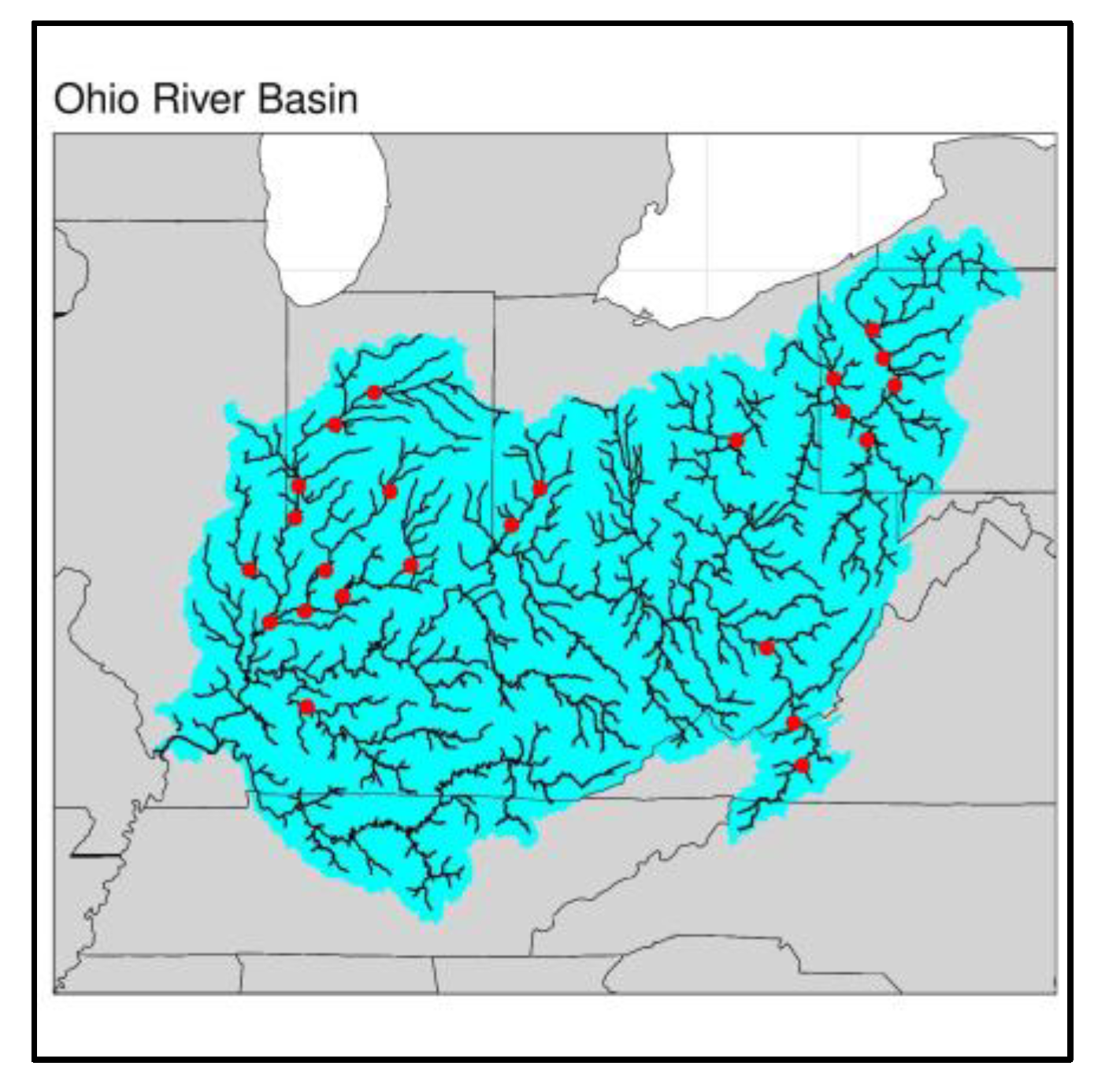
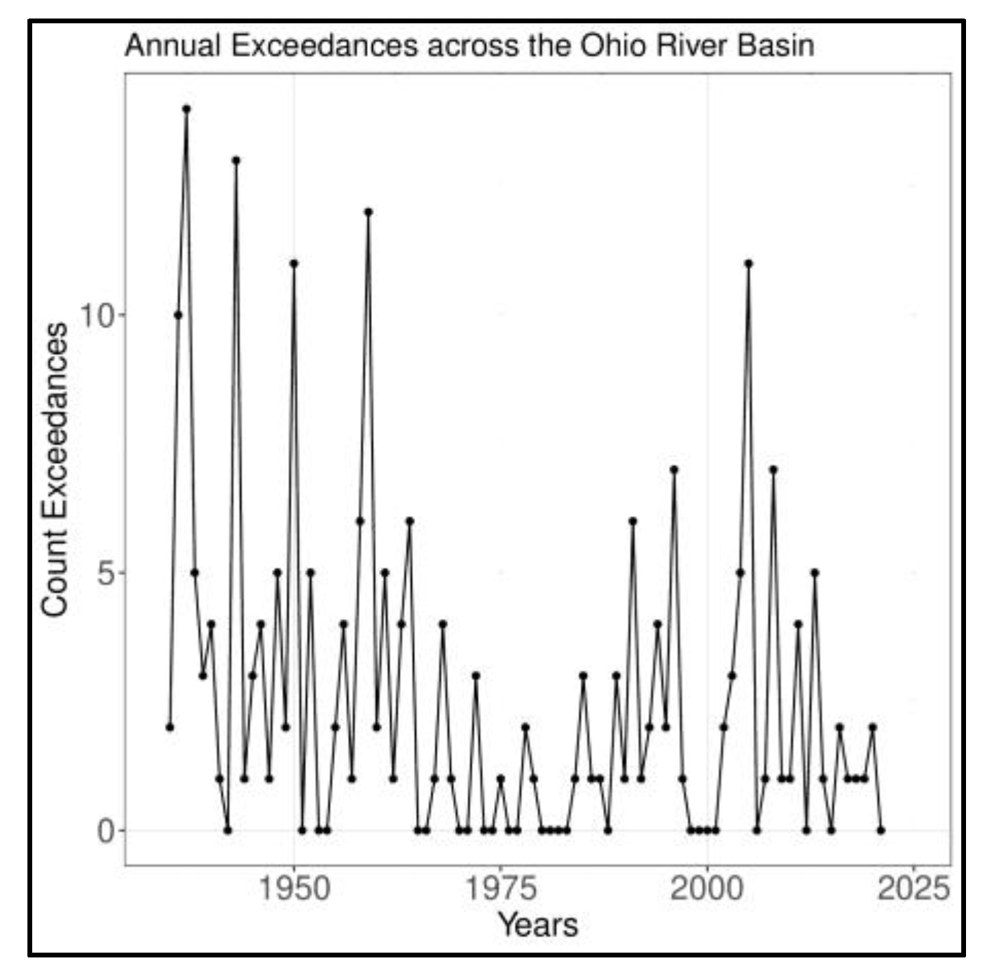
2.1. Streamflow Data

The daily streamflow data were downloaded from the United States Geological Survey (USGS) water databases using the ‘dataRetrieval’ package [36]. Stream gauges located in the Ohio river basin with a maximum of 0.1% of missing data and a drainage area greater than 3750 sq. miles were selected. Sites with a significant regulation of flow during the period of study affecting the annual maxima were not considered. Using the above criteria, 24 sites (Figure 1) were included in this study, with each location having 87 years of data from 1935–2021. The daily streamflow time series at each site was used to identify the annual maximum streamflow for each water year, which started in October (1/10) of the previous year and ended in September (30/9) of the current year.

2.2. Climate Indices

Climate indices are time series of diagnostic quantities that are used to characterize hydro-climatic systems based on data from climate stations, grid points, regional averaged data, or computed from empirical orthogonal functions and usually involve a single field, most commonly sea surface temperature anomalies [37]. The most commonly used climate indices are the El Niño Southern Oscillation index, Pacific Decadal Oscillation, North Atlantic Oscillation, and Atlantic Multi-decadal Oscillation.

The Niño 3.4 index, used as an indicator of the El Niño Southern Oscillation phenomena as the dominant mode of global variability influencing climate globally, is computed from sea surface temperature anomalies in the equatorial Pacific [38]. The Pacific Decadal Oscillation (PDO) index is computed as the first principal component of the Northern Pacific sea surface temperature anomalies [17,39]. The Atlantic Multidecadal Oscillation (AMO) is computed from the sea surface temperature anomalies in the northern Atlantic basin [40]. The North Atlantic Oscillation (NAO) index, unlike the above-mentioned indices, is computed as the surface sea-level pressure difference between the subtropical high (Azores or Gibraltar) and the sub-polar low (Iceland) [41].

The Niño 3.4, NAO, PDO, and AMO indices were converted from monthly resolution to annual time-scale by computing their mean Dec–Jan–Feb values, which corresponded to boreal winter. This seasonal choice was made since most of the extreme floods in the basin occur in the January–April period. They were standardized before use in this study. Interactions between the indices were computed as the product of departures from their respective means.

$${xy}_t=\left(x_t-\overline{x}\right)\times (y_t-\overline{y})$$

(1)

where $x_t$, $y_t$, and ${xy}_t$ are the values of the climate indices x, y, and their interaction at time t, respectively. $\overline{x}$ and $\overline{y}$ are the mean values of climate index x and y, respectively. The KNMI Climate Explorer (https://climexp.knmi.nl/start.cgi (accessed on 10 October 2022)) was used as the primary data extraction source for these indices. Overall, ENSO, NAO, PDO, and AMO, along with their interactions, were used in this study, where their connections to the leading modes of streamflow variability within the Ohio River Basin that are identified were explored. Double labels, for example, ENSO–NAO, denote interactions between ENSO and NAO.

3. Methods

We considered two complementary strategies for the diagnosis of multi-site low-frequency variations and their associated space-time signatures in basin-wide annual maximum streamflow. From a regional perspective, we hypothesized that the time series at all sites could be modulated at the same frequencies if they were influenced by larger-scale climate oscillations that have marked quasi-periodic variability. Such common large-scale drivers can also induce a spatial correlation structure in the annual maxima flow series across the sites, even if the flows do not occur simultaneously across all the sites in each year. All the larger extreme floods occur in the same season and often correspond to recurrent synoptic waves of incoming atmospheric moisture every 4–7 days [33,34]. Thus, some sites may experience the annual maximum event earlier than others, while all sites have elevated flows in such a season. Two complementary approaches were explored to diagnose the multi-site low-frequency variations and spatiotemporal structure in annual maxima streamflow: (1) PC-Wavelet and (2) Wave-Clust (Figure 3).

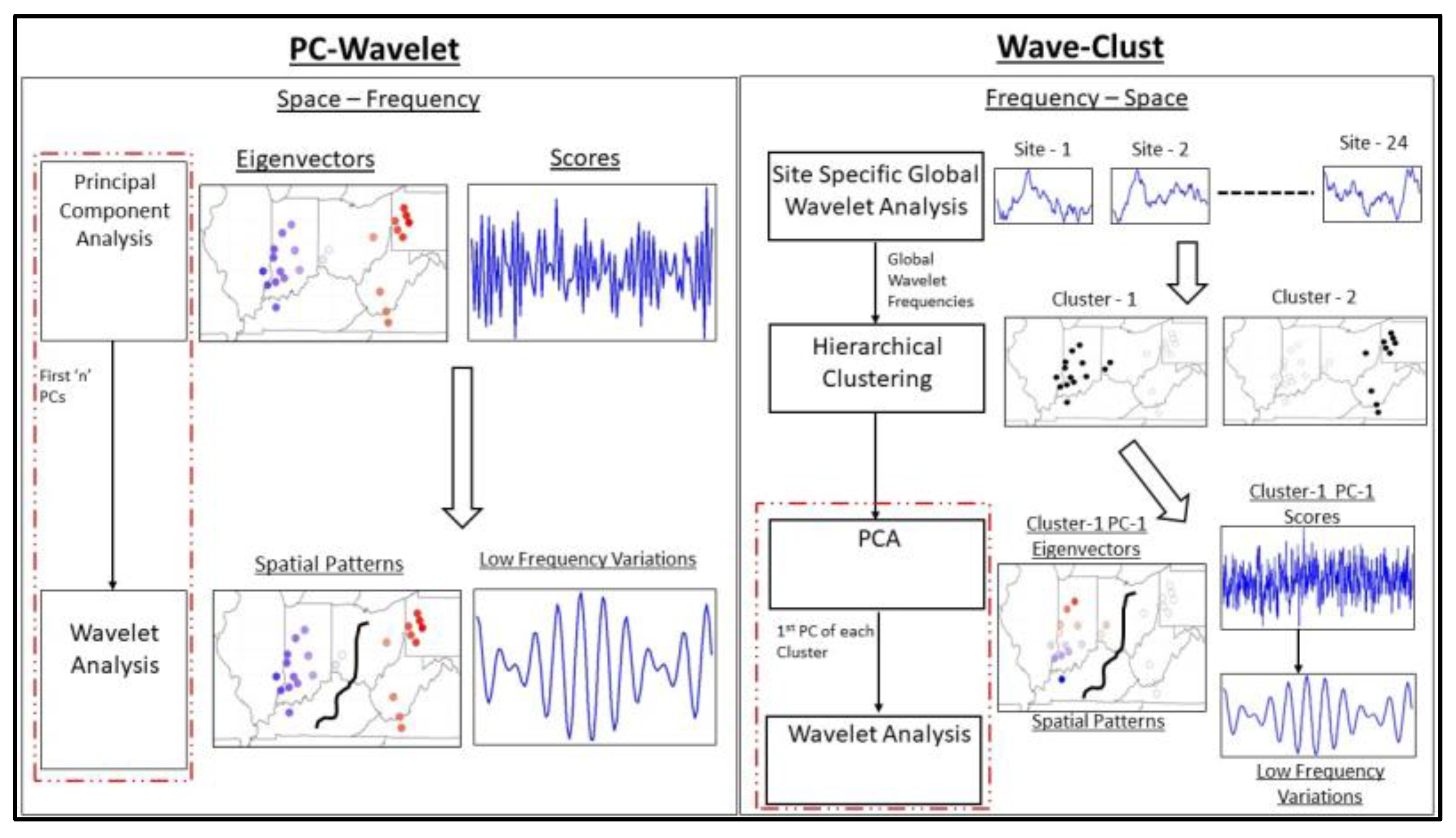
3.1. PC-Wavelet

The PC-Wavelet method (Figure 3 (left)) corresponds to a method that analyzes the spatial structure of the multi-site data followed by a time-frequency analysis of the resulting spatial patterns. A principal component analysis (PCA) [42] was performed on a correlation matrix of the annual maxima streamflow data across the 24 sites to achieve a reduction in the spatial dimension. The eigenvectors of the leading principal components identified the patterns of spatial variability. The number of leading principal components to be analyzed was decided by the variance (eigenvalues), as explained by the PCs. Each leading PC was then subjected to wavelet analysis to identify the common low-frequency variations across time if any. The following sub-section can be referred to for further details on wavelet analysis.

3.2. Wave-Clust

The first step of the Wave-Clust method (Figure 3 (right)) entails wavelet analysis on the annual maxima streamflow time series of the 24 sites, followed by the hierarchical clustering of the resulting wavelet transforms. Hierarchical clustering, a form of agglomerative clustering, was used to partition objects in a set based on measures of similarity, with the most common being the distance between the objects [43]. In this study, ‘Ward Distance’, which minimizes the within-cluster variance, was used as the distance measure for cluster separation [44]. The hierarchical clustering was applied to the time-varying wavelet power across each of the frequencies/scales at each site. The hierarchical cluster analysis on the time-frequency structure helped identify clusters that participated in similar climate patterns but were not necessarily orthogonal or statistically independent. The selection of the number of clusters to use was performed through a visual inspection of the dendrogram and the dissimilarity measure. Once the spatial clusters were identified, we performed a PCA on only the time series in the cluster and examined the time-frequency structure of the leading PC using wavelet analysis to identify the dominant time-frequency mode for that cluster. The eigenvectors and principal component scores for the first principal component for each cluster gave the spatial dependence structure and temporal variation within that cluster, respectively.

Figure 3 shows a schematic of this method, with an explicit east–west clustering divide and the identification of low-frequency signals from the leading principal component of a cluster by means of wavelet analysis. The space-time patterns identified from PC-Wavelet may or may not be similar to those identified from the Wave-Clust, and consequently, they may exhibit different relations to the larger-scale climate indices. The wavelet analysis, which is a building block of both the PC-Wavelet and Wave-Clust methods, is summarized below.

Wavelet Analysis

Wavelet analysis was used as a tool to analyze the localized power variations in a time series. We applied it here to analyze the time-frequency structure in the annual maximum streamflow series at each site and also for each PC. The presentation below follows [45], where the continuous wavelet transform (CWT) of the discrete-time series $x_t$ of length N (t = 0 to N − 1), with discrete time spacing, $\delta t$ is defined by:

$$W_t\left(\mathrm{s}\right)=\sum _{t^{’}=0}^{N-1}{x}_{t^{\prime }}{\psi }^{*}\left[\frac{(t^{\prime }-t)\delta t}{s}\right]$$

(2)

where ${\psi }^{*}$ is the complex conjugate of the wavelet function ${\psi }^{}$, and s is the wavelet scale. The Morlet wavelet function was utilized in this study. The wavelet function $\psi \left(t\right)$ is complex, i.e., it has a real and an imaginary part. The variations in the wavelet scale s and translations along the localized time index allow for the analysis of both the change in amplitude versus scale and the change in amplitude versus time. A faster method to compute the wavelet transform is via calculations in Fourier space, and to approximate the continuous wavelet transform, a convolution at each scale s was conducted N times. By using the convolution theorem, the continuous wavelet transform is the inverse Fourier transform of the product [45] given by

$$W_t\left(\mathrm{s}\right)=\sum _{k=0}^{N-1}\widehat{x_k}\widehat{{\psi }^{*}}\left(s{\omega }_k\right)e^{i{\omega }_{k}t\delta t}$$

(3)

where $\widehat{x_k}$ is the discrete Fourier transform of $x_{it}$, and ${\omega }_k$ is the angular frequency. The wavelet transform $W_t\left(\mathrm{s}\right)$ is complex and can be divided into real and imaginary parts. The wavelet power spectrum is defined as the square of its amplitude and is given by ${\left|W_t\left(\mathrm{s}\right)\right|}^2$. The significance level associated with the wavelet spectrum is tied explicitly to the choice of background spectrum, which for hydro-climatic data, is often taken to be a red noise or white noise spectrum. The red noise significance test developed by [45] involves fitting an AR(1) model to the time series and computing its Fourier spectrum where the associated one-sided (1 − α)% confidence limits give the α% significance levels over red noise at the scale. We guide the reader to [45] for details.

For the Wave-Clust, at each site i, the annual maximum flood series $x_{it}$ is transformed into $W_{ti}\left(\mathrm{s}\right)$ as above, and the hierarchical clustering method is used to divide the sites i = 1… ns into sub-groups based on the similarity of the $W_{ti}\left(\mathrm{s}\right)$. For the PC-Wavelet analysis, the time series of a principal component is used as $x_{it},$ and the resulting $W_t\left(\mathrm{s}\right)$ is examined for significant variance at each scale s.

3.3. Diagnostic Analysis of the Role of Low Frequency Climate Variation

The climate indices ENSO, NAO, PDO, AMO, and their interactions with the global annual temperatures, are considered potential candidates which influence streamflow variability within the Ohio River Basin. We analyzed the relationship of these climate indices with the leading modes identified from the PC-Wavelet or Wave-Clust. These relationships were analyzed first through correlation analysis, followed by linear and non-linear regression methods. A further description of these methods is provided below.

3.3.1. Correlation Analysis

Wavelet coherence is used to assess the relationship between the dominant modes of variability in the annual maximum streamflow data and the known global or hemispheric modes of atmospheric variability [45,46]. The wavelet coherence $R_t^2$ is defined as:

$$R_t^2=\frac{{\left|S\left(s^{-1}{W}_t^{xy}\right(s\left)\right)\right|}^2}{S\left(s^{-1}{\left|W_t^x\left(s\right)\right|}^2\right)S\left(s^{-1}{\left|W_t^y\left(s\right)\right|}^2\right)}$$

(4)

$$W_t^{xy}=W_t^x{W}_t^{y*}$$

(5)

where $W_t^x$ is the continuous wavelet transform of $x_t$ and ‘*’ denotes the complex conjugate of $W_t^y$, which is the continuous wavelet transform of $y_t$; S is a smoothing operator, and s is the scale. The wavelet coherence can be thought of as a localized correlation between two-time series in the time-frequency domain, with the above equation resembling a correlation coefficient equation. We refer the reader to [45,46] for further details on this method. The wavelet coherences were computed and generated using the ‘biwavelet’ package in R [47]. Furthermore, we also looked at the direct correlation between the PCs and the climate indices using the Pearson correlation coefficient [48].

3.3.2. Linear Regression with Regularization and Variable Selection

The least absolute shrinkage and selection operator (LASSO) is a linear regression method that performs both regularization and variable selection [49]. Lasso is a penalized selection method that minimizes the residual sum of squares, which is subject to the sum of the absolute value of the coefficients and is less than a constant [50]. The coefficients ${\beta }_j$ of the linear relationship between a response variable Y_i and p predictors X_ij were solved by minimizing the cost function:

$$\sum _{i=1}^n{\left(Y_i-\sum _{j=1}^p{X}_{ij}{\beta }_j\right)}^2+\lambda \sum _{j=1}^p\left|{\beta }_j\right|$$

(6)

where, $\lambda \ge 0$ is the shrinkage parameter.

This is subject to the constraint:

$${\sum }_j\left|{\beta }_j\right|\le \mathrm{t}$$

(7)

The parameter $\lambda$ controls the magnitude of shrinkage that is applied to the model and is selected using leave-one-out cross-validation. This formulation leads to a sparse solution where several of the coefficients ${\beta }_j$ are set to zero if the corresponding predictor does not contribute significantly to the dependent variable. This translates into an automatic variable selection. This analysis was carried out using the glmnet package [51] in R.

3.3.3. Non-Linear Regression

Random forests are a class of ensemble learning methods that use decision trees as the building blocks [52]. They can be used for either classification or in a regression setup. In a regression setup, the mean of the predictions across the ensemble of decision trees is used as the estimate.

A random forest consists of an ensemble of decision trees, where each tree is constructed using a bootstrapped (sampling with replacement) sample of the data. The CART algorithm is then used to train the decision trees. In addition to the bootstrap, a subset of the variables is selected at random, and the best split is based on that limited subset only (52). Since the input training data for each tree are drawn at random, and a subset of the variables are used for node splitting, random forests overcome the issue of overfitting and the high variance faced by modeling individual decision trees. The bootstrapping of the training data, leaving out a fraction of the data that is not used for training that decision tree, is then used to compute the out-of-bag estimate, thereby providing validation in spite of using the entire data to train the algorithm.

Random forest models allow for the computation of a variable importance measure, which can be used to perform variable selection or identify relevant variables/features. The variable importance is decided using the Gini impurity criterion [53]. The ’RandomForest’ [54] package in R is used to fit these models.

4. Results

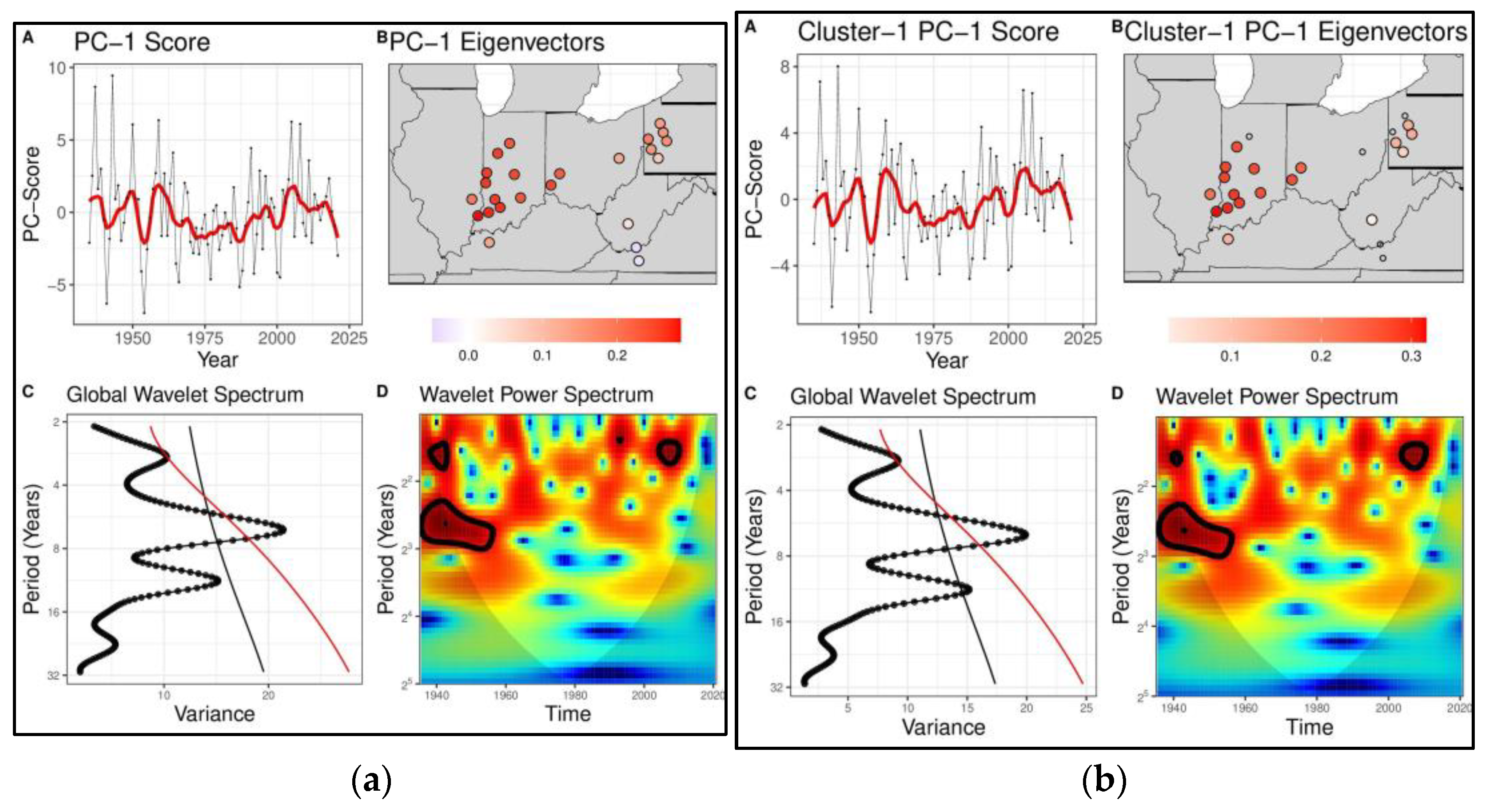
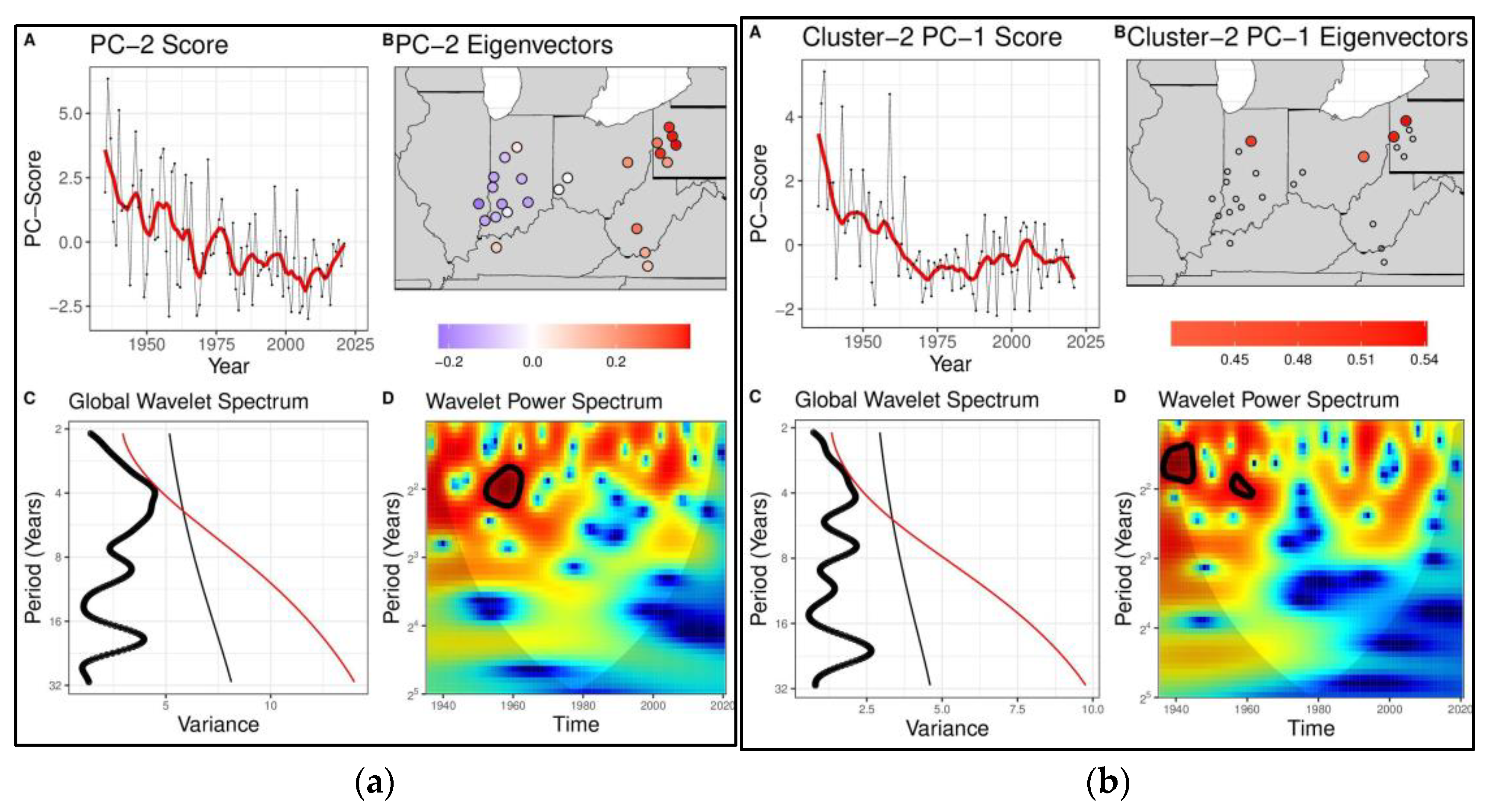
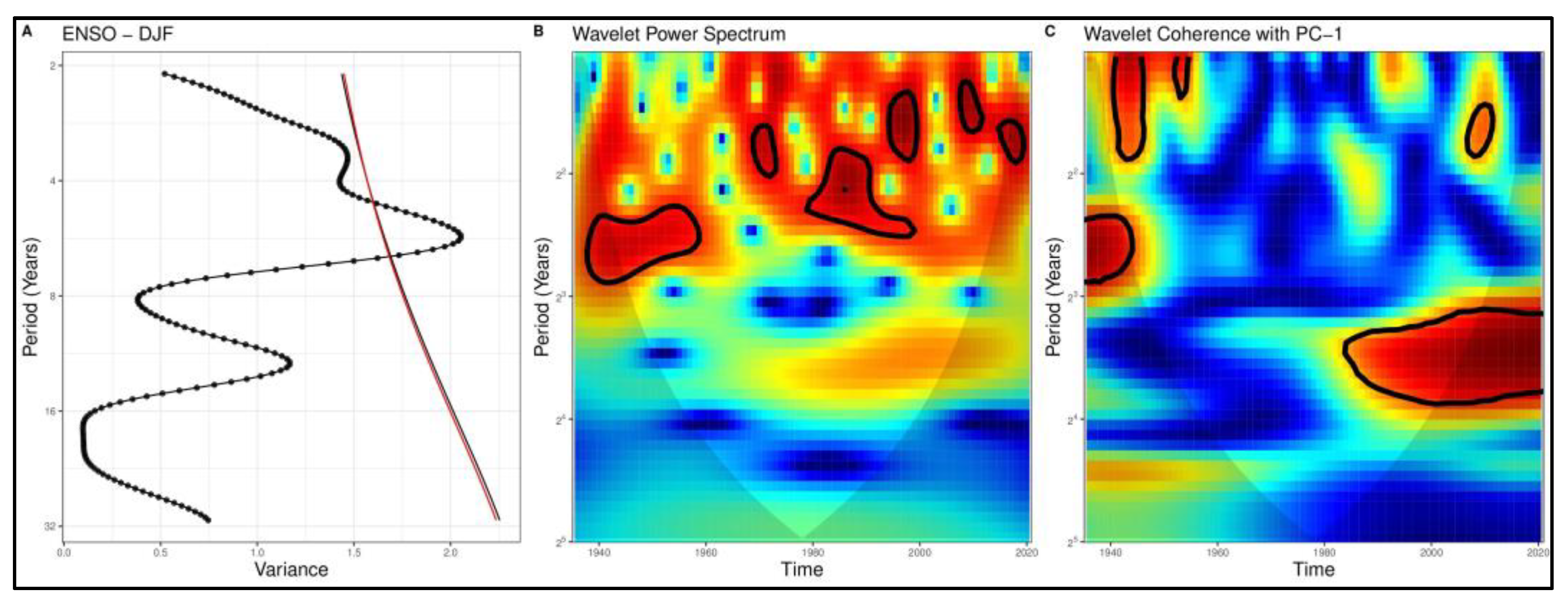
4.1. Diagnosis of Low Frequency Variations and Space-Time Signatures for the ORB

The PC-Wavelet and Wave-Clust methods were applied to the annual maximum streamflow data across the Ohio river basin to identify the low-frequency variations and space-time signatures of the data (Figure 4 and Figure 5). The first and second principal components of annual maximum streamflow data explain ~39% and 16% of the total variance, respectively, adding up to 56% of the total variance (Figure A1). Hierarchical clustering, when applied to the wavelet-transformed streamflow data, led to the identification of two primary clusters among the stream gauges (Figure A2). The leading two principal components and the two clusters from the Wave-Clust were subsequently analyzed further. The two methods led to consistent results in the identification of the dominant space-time frequency structure of floods for the leading PC (Figure 4) but diverged for the second dominant mode of variability (Figure 5).

Figure 4 and Figure 5 show the application of the PC-Wavelet and Wave-Clust methods to the leading and second dominant mode of variability affecting the annual maxima streamflow within the Ohio River Basin. For PC1, the associated spatial pattern reflected a positive correlation across all but two of the southeastern gauges. Focusing on the temporal domain, the wavelet spectrum for PC-1 of the entire field (Figure 4(a-C)) and for the first wavelet cluster (Figure 4(b-C)) showed a sharp peak around 6–7 years, which was statistically significant at the 90% level relative to a red noise null hypothesis. This finding was particularly evident pre-1960 (sub-panel D). Visually, the time series (sub-panel A) exhibited a much higher variance pre-1970 than in the 1970–1990 period. Episodic variability organized over an approximately three-year period was also seen to be statistically significant at the 90% level relative to the red noise null hypothesis. The second principal component from PC-Wavelet (Figure 5a) and the leading PC of the second largest cluster (Figure 5b) both contained large secular trends. The 1930s–1960s are periods characterized by a large number of exceedances (Figure 2) and where the wavelet power spectrum is significant (Figure 4(a-D,b-D)). It also shows that large regions have similar spectral signatures, possibly pointing to regions that have similar dynamics or are forced by global external climatic variability.

The leading mode captures the dynamics of the aggregate (lower Ohio) basin with a key 6–7-year periodicity and a weaker 12-year cycle (Figure 4). The second mode highlights the eastern-western divide within the basin with few characteristic low-frequency variations but also indicates the presence of a strong trend. This secular trend could be modulated by an extremely low-frequency variation or anthropogenic climate change. It is likely to be related to a systematic displacement west of the meridional moisture flow from the Gulf of Mexico coming into the Ohio River Basin [55,56].

Overall the order of processing space-time (PC-Wavelet) or time-space (Wave-Clust) can lead to different insights. For PC1 and cluster 1, the difference is small because the same dominant pattern was identified, and the dominant cluster had 18 (out of 24) stations representing the group’s frequency behavior. The PC1 eigenvectors suggest that this is more or less the average spatial behavior across the sites since they are all of the same sign. The differences across sites are in the eigenvector coefficients, representing the varying degree of participation in the regional pattern. In this case, the inter-annual modes are identified as the regional feature by the space-time (PC-Wavelet) analysis. Correspondingly, the stations that participated the most in the same frequency structure are identified as the dominant cluster by the time-space (Wave-Clust) analysis.

However, since the clustering process is disjunctive, in that stations assigned to cluster 1 cannot show up in cluster 2, the second cluster now represents a much smaller set of stations, and the dominant feature in these stations emerges as a secular trend or shift. By this time-space (Wave-Clust) method, this shift is associated with just these four stations.

However, by looking at the space-time (PC-Wavelet) analysis, we can see that the corresponding PC-2 actually exhibits a spatial pattern that has a dipole structure, and in conjunction with the trend in the time series, we understand that this is also a regional pattern with a secular trend that indicates a post-1960 decline in the flood magnitudes in the Eastern part of the basin relative to the Western part of the basin. The time series of the PC-2 and the average of Cluster 2 are similar, with the only difference being that cluster 2 has a minimal inter-annual variability, and the long-term trend dominates.

4.2. Diagnosis of Relations with Climate Indices

As hypothesized earlier, large-scale climate drivers may induce a spatiotemporal structure in the annual maxima streamflow series across sites, even if the flows do not occur simultaneously across all the sites in each year. The large-scale climate indices considered were ENSO, PDO, NAO, AMO, and their interactions with each other. We also included the lagged annual global temperature as a proxy of the long-term climate trend due to anthropogenic climate change. Overall, we explored the possibility of the joint influence of global climate variability through these climate indices in addition to the climate change signal, which influenced the climate indices. Since the modes computed from the PC-Wavelet and Wave-Clust are similar and PC-Wavelet represented the entire region, the modes computed from PC-Wavelet were retained for subsequent analysis.

4.2.1. Correlation Analysis

The leading modes of streamflow variability within the Ohio River Basin were first analyzed to explore the influence of hemispheric climate variability through climate indices and the long-term global warming trend. The leading principal component (PC-1), which explains 39% of the total variance, is the dominant mode of the regional flow variability. It has a significant Pearson correlation coefficient with only ENSO (r = −0.27) at the 5% level (Figure 6). PC-1’s correlation with other indices, including temperature, which serves as a proxy for the anthropogenic climate trend, is low and non-significant. Figure 6 provides the correlation values between PC-1, PC-2, and other climate indices.

In the time-frequency domain, PC-1 has a strong peak in variance near the 6–7-year band, which is significant at the 10% level relative to a hypothesis of red or white noise, along with a weaker and lower frequency of a 12-year cycle (Figure 4(a-C)). The global wavelet spectrum of the Niño 3.4 index (ENSO) averaged over Dec-Jan-Feb shows elevated variance associated with the 5–7 year band, which is significant at the 10% level, a key characteristic of the ENSO phenomenon, along with a weaker 12–14 year periodicity (Figure 7A). The power associated with the 5–7 year interannual band was highest in the broad periods of our data records (1940–1960, 1980–2000) (Figure 7B). The wavelet coherence between PC-1 and the ENSO index showed high coherency in the 12-year cycle post-1980s and was significant at the 10% level (Figure 7C), which is suggestive of a connection between the two. Further, the phase angle indicates that ENSO leads PC-1 by a period of 1 year at this frequency.

The second principal component PC-2, which explains 16% of the total variance in annual maxima streamflow variability, was characterized by a long secular trend (Figure 5(a-a-C)). PC-2 has high correlations with NAO (r = −0.26), PDO-AMO (r = 0.28), and temperature (r = −0.43), all of which are significant at the 5% level (Figure 6). Overall, the nature of the trend in PC-2, which filters information on the east–west divide, mirrors to a large degree the long-term trend in temperature that is driven by anthropogenic warming.

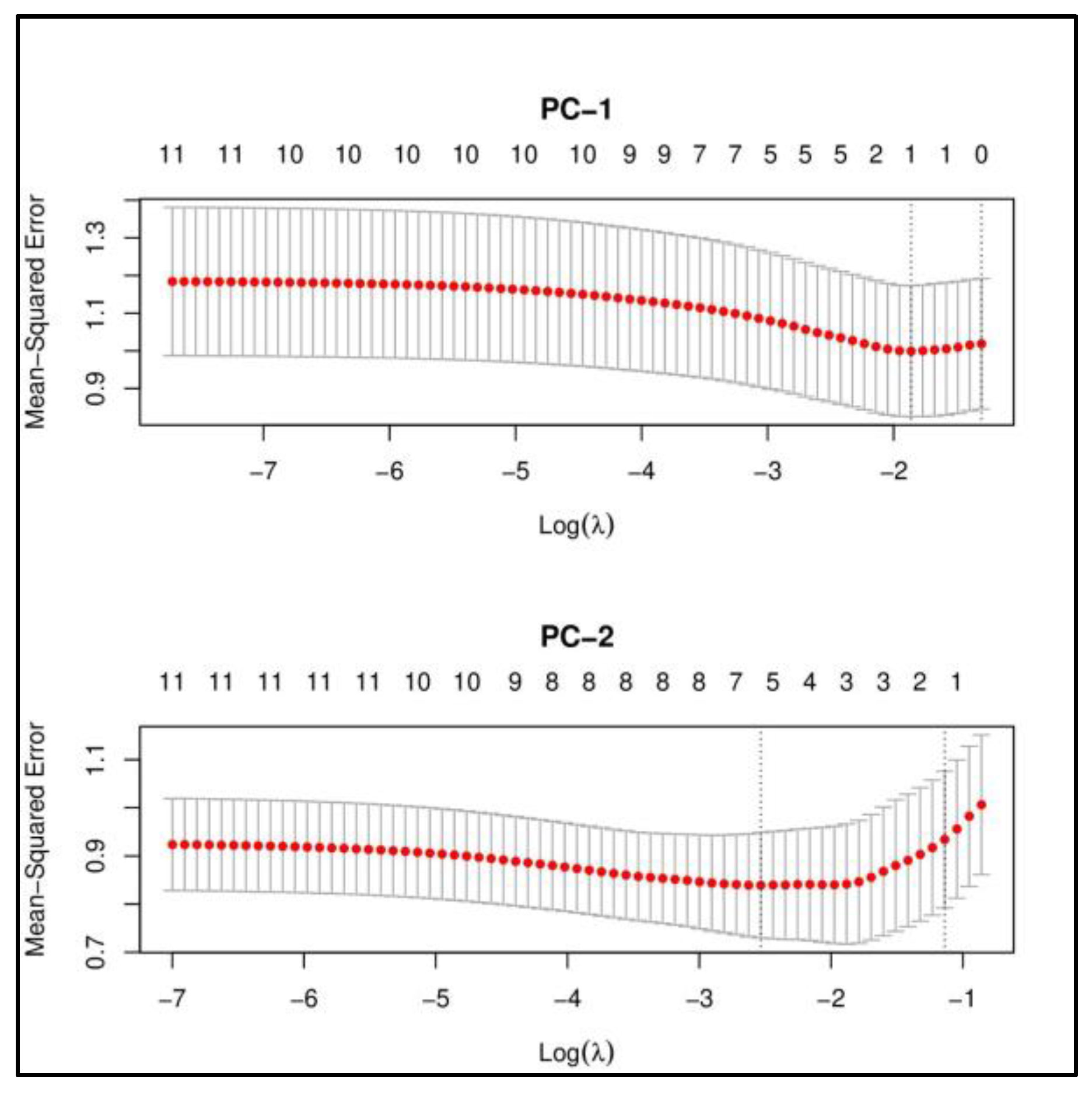
4.2.2. Linear Regression

Figure 8 (top) shows the cross-validated results for lasso regression with PC-1 as the dependent variable and the climate indices with their interactions and temperature as the independent variables. ENSO is the only variable selected, whereas the coefficients of all other variables are pushed to zero when the cross-validated mean squared error is the lowest. This corresponds to the dashed line in Figure 8 (top). Furthermore, the removal of the other ten variables leads to a decrease in the cross-validated error, indicating that no linear combination of any subset for the non-ENSO variables is useful for predicting PC-1.

Lasso regression with PC-2 as the dependent variable results in the inclusion of multiple variables for the lowest cross-validated error. Temperature, PDO, NAO, AMO, and PDO-AMO are the selected variables when the shrinkage penalty is log(λ) ≈ −2.5. The other dotted line (log(λ) ≈ −1) to the right in Figure 8 (bottom) corresponds to the largest value of the shrinkage parameter (most parsimonious with the least number of predictors) such that the value of the cross-validated error is within one standard deviation of the minimum error. This scenario includes only temperature as the independent variable, with all others, pushed to zero, highlighting the role of temperature as the most important variable in this subset for predicting PC-2.

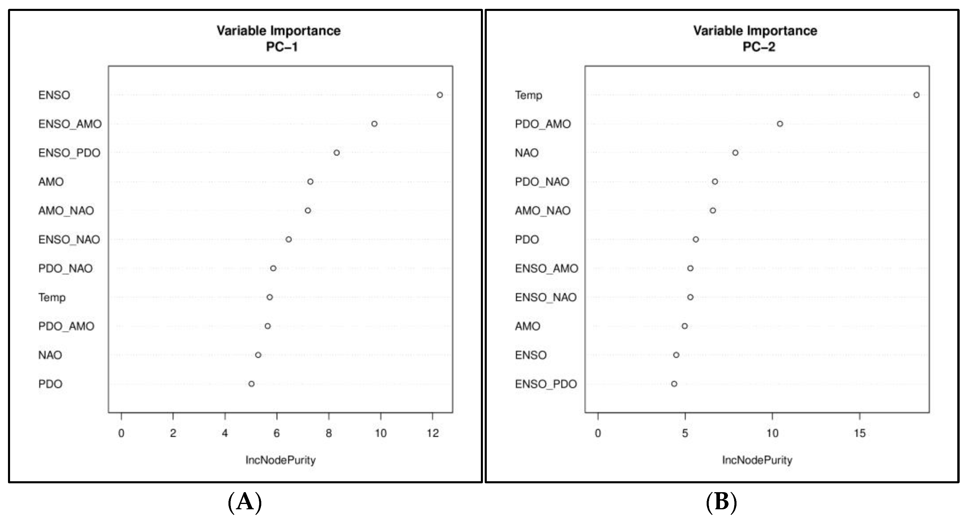
4.2.3. Non-Linear Regression

Random forest models were fit separately with PC-1 and PC-2 as dependent variables. Each model was fit with 10,000 individual trees, and $\sqrt{11}\approx 3$ variables were used at each split. The models, as non-linear regression counterparts of the lasso, were used to identify a subset of pertinent variables to the dependent variables.

Figure 9A denotes variable importance when PC-1 is used as a dependent variable in a random forest regression setting. ENSO came up as the most important variable in this case, followed by ENSO-AMO and ENSO-PDO. The temperature showed up as the most important variable when PC-2 was the dependent variable (Figure 9B). This was followed by PDO-AMO, NAO, PDO-NAO, and AMO-NAO, which had similar levels of importance.

Overall, given the regression analysis on climate indices in addition to the diagnostic analysis, our interpretation is that the region has two dominant modes of long-term variability. The leading principal component PC-1 is associated with ENSO and marked by inter-annual variability, and it seems to have a basin-wide impact. The second leading mode, PC-2, is characterized by a long secular trend, and its primary climate association appears to be with the global warming trend, with a possible association identified between some of the lower frequency climate indices. PC-2 reflects a west–east shift in the incidence of flooding since the 1960s and correlated best with global annual temperature. If indeed this is due to anthropogenic climate change-induced global warming, then it is an interesting observation indicating a spatial shift in the sub-basins that are likely to be flooded.

5. Summary

This paper was motivated by the need to better understand compound flood risks at the river basin scale in terms of the potential for spatial and temporal clustering of floods. We noted that the temporal pattern of the number of annual exceedances for the 10-year return period annual maximum flood at the 24 sites was extremely unlikely to have occurred by chance if the data indeed included spatially and temporally independent random variables. This begged the question of whether there were spatial patterns of flooding with distinct quasi-periodic or secular trends that could be related to large-scale climate variability, including anthropogenic global climate change.

Recognizing that the answer to this question may be sensitive to whether we first identified dominant spatial patterns and then looked at the time-frequency structure or if we identified the time-frequency structure at each site and then looked for spatial similarities in those patterns, we used the PC-Wavelet and the Wave-Clust methods to decompose the space-time-frequency structure in the 24-time series. For the leading modes of variability that accounted for about 56% of the spatial correlation in the flood occurrence process, we found that the order of processing space-time or time-space made a difference in the insights that could be drawn. The leading PC represents a common behavior across the Ohio River Basin with quasi-periodic variability at the inter-annual and decadal time scales that appeared to be associated with similar variability in the ENSO index. The second PC represented an east–west dipole or negative correlation that was associated with a pronounced secular trend and appeared to be associated most strongly with the global temperature index reflecting a shift in the likelihood of flooding from the eastern to the western part of the basin. This is an interesting find that reinforces not just increased moisture in the atmosphere due to warming but subtle shifts in circulation modes, which lead to spatial shifts in flood occurrence that may be of considerable interest for researchers to understand as they project future flood risks, especially from a compound risk perspective; this translates into a need to better understand the spatial structure of flood incidence over the entire flood season in a regional context of the larger river basin. The analysis also highlights the need to develop statistical methods for the multi-scale conditioning of compound extremes accounting for the slower climate variations that induce synoptic event structures that favor such clustering.

References

- Merz, B.; Blöschl, G.; Vorogushyn, S.; Dottori, F.; Aerts, J.C.J.H.; Bates, P.; Bertola, M.; Kemter, M.; Kreibich, H.; Lall, U.; et al. Causes, impacts and patterns of disastrous river floods. Nat. Rev. Earth Environ. 2021, 2, 592–609. [Google Scholar] [CrossRef]
- Pielke, R.A., Jr.; Gratz, J.; Landsea, C.W.; Collins, D.; Saunders, M.A.; Musulin, R. Normalized hurricane damage in the United States: 1900–2005. Nat. Hazards Rev. 2008, 9, 29–42. [Google Scholar] [CrossRef]
- Peduzzi, P.; Chatenoux, B.; Dao, H.; De Bono, A.; Herold, C.; Kossin, J.; Mouton, F.; Nordbeck, O. Global trends in tropical cyclone risk. Nat. Clim. Chang. 2012, 2, 289–294. [Google Scholar] [CrossRef]
- Merz, B.; Aerts, J.; Arnbjerg-Nielsen, K.; Baldi, M.; Becker, A.; Bichet, A.; Blöschl, G.; Bouwer, L.M.; Brauer, A.; Cioffi, F.; et al. Floods and climate: Emerging perspectives for flood risk assessment and management. Nat. Hazards Earth Syst. Sci. 2014, 14, 1921–1942. [Google Scholar] [CrossRef] [Green Version]
- Kemter, M.; Merz, B.; Marwan, N.; Vorogushyn, S.; Blöschl, G. Joint Trends in Flood Magnitudes and Spatial Extents across Europe. Geophys. Res. Lett. 2020, 47, e2020GL087464. [Google Scholar] [CrossRef] [PubMed] [Green Version]
- Bonnafous, L.; Lall, U.; Siegel, J. A water risk index for portfolio exposure to climatic extremes: Conceptualization and an application to the mining industry. Hydrol. Earth Syst. Sci. 2017, 21, 2075–2106. [Google Scholar] [CrossRef] [Green Version]
- Jain, S.; Lall, U. Floods in a changing climate: Does the past represent the future? Water Resour. Res. 2001, 37, 3193–3205. [Google Scholar] [CrossRef]
- Lun, D.; Fischer, S.; Viglione, A.; Blöschl, G. Detecting Flood-Rich and Flood-Poor Periods in Annual Peak Discharges across Europe. Water Resour. Res. 2020, 56, e2019WR026575. [Google Scholar] [CrossRef]
- Haraguchi, M.; Lall, U. Flood risks and impacts: A case study of Thailand’s floods in 2011 and research questions for supply chain decision making. Int. J. Disaster Risk Reduct. 2015, 14, 256–272. [Google Scholar] [CrossRef]
- Bonnafous, L.; Lall, U. Space-time clustering of climate extremes amplify global climate impacts, leading to fat-tailed risk. Nat. Hazards Earth Syst. Sci. 2021, 21, 2277–2284. [Google Scholar] [CrossRef]
- Swierczynski, T.; Brauer, A.; Lauterbach, S.; Martin-Puertas, C.; Dulski, P.; von Grafenstein, U.; Rohr, C. A 1600 yr seasonally resolved record of decadal-scale flood variability from the Austrian Pre-Alps. Geology 2012, 40, 1047–1050. [Google Scholar] [CrossRef]
- Meko, D.M.; Woodhouse, C.A. Tree-ring footprint of joint hydrologic drought in Sacramento and Upper Colorado river basins, western USA. J. Hydrol. 2005, 308, 196–213. [Google Scholar] [CrossRef]
- Ropelewski, C.F.; Halpert, M.S. Global and Regional Scale Precipitation Patterns Associated with the El Niño/Southern Oscillation. Mon. Weather Rev. 1987, 115, 1606–1626. [Google Scholar] [CrossRef]
- Ward, P.J.; Jongman, B.; Kummu, M.; Dettinger, M.D.; Weiland, F.C.S.; Winsemius, H.C. Strong influence of El Niño Southern Oscillation on flood risk around the world. Proc. Natl. Acad. Sci. USA 2014, 111, 15659–15664. [Google Scholar] [CrossRef] [Green Version]
- Ward, P.J.; Beets, W.; Bouwer, L.M.; Aerts, J.C.J.H.; Renssen, H. Sensitivity of river discharge to ENSO. Geophys. Res. Lett. 2010, 37, L12402. [Google Scholar] [CrossRef] [Green Version]
- Olsen, J.R.; Stedinger, J.R.; Matalas, N.C.; Stakhiv, E.Z. Climate Variability and Flood Frequency Estimation for the Upper Mississippi and Lower Missouri Rivers. JAWRA J. Am. Water Resour. Assoc. 1999, 35, 1509–1523. [Google Scholar] [CrossRef]
- Mantua, N.J.; Hare, S.R.; Zhang, Y.; Wallace, J.M.; Francis, R.C. A Pacific Interdecadal Climate Oscillation with Impacts on Salmon Production. Bull. Am. Meteorol. Soc. 1997, 78, 1069–1080. [Google Scholar] [CrossRef]
- Toomey, M.; Cantwell, M.; Colman, S.; Cronin, T.; Donnelly, J.; Giosan, L.; Heil, C.; Korty, R.; Marot, M.; Willard, D. The Mighty Susquehanna—Extreme Floods in Eastern North America During the Past Two Millennia. Geophys. Res. Lett. 2019, 46, 3398–3407. [Google Scholar] [CrossRef] [Green Version]
- Hodgkins, G.A.; Whitfield, P.H.; Burn, D.H.; Hannaford, J.; Renard, B.; Stahl, K.; Fleig, A.K.; Madsen, H.; Mediero, L.; Korhonen, J.; et al. Climate-driven variability in the occurrence of major floods across North America and Europe. J. Hydrol. 2017, 552, 704–717. [Google Scholar] [CrossRef] [Green Version]
- Stedinger, J.R., Jr.; Cohn, T.A.; Faber, B.A.; England, J.F.; Thomas, W.O., Jr.; Veilleux, A.G.; Kiang, J.E.; Mason, R.R., Jr. Guidelines for Determining Flood Flow Frequency—Bulletin 17C; U.S. Geological Survey: Reston, VA, USA, 2019. [Google Scholar]
- Milly, P.C.D.; Betancourt, J.; Falkenmark, M.; Hirsch, R.M.; Kundzewicz, Z.W.; Lettenmaier, D.P.; Stouffer, R.J. Stationarity Is Dead: Whither Water Management? Science 2008, 319, 573–574. [Google Scholar] [CrossRef]
- Filho, F.D.A.S.; Lall, U. Seasonal to interannual ensemble streamflow forecasts for Ceara, Brazil: Applications of a multivariate, semiparametric algorithm. Water Resour. Res. 2003, 39, 1307. [Google Scholar] [CrossRef]
- Grantz, K.; Rajagopalan, B.; Clark, M.; Zagona, E. A technique for incorporating large-scale climate information in basin-scale ensemble streamflow forecasts. Water Resour. Res. 2005, 41, W10410. [Google Scholar] [CrossRef]
- Regonda, S.K.; Rajagopalan, B.; Clark, M.; Zagona, E. A multimodel ensemble forecast framework: Application to spring seasonal flows in the Gunnison River Basin. Water Resour. Res. 2006, 42, W09404. [Google Scholar] [CrossRef] [Green Version]
- Towler, E.; Rajagopalan, B.; Gilleland, E.; Summers, R.S.; Yates, D.; Katz, R. Modeling hydrologic and water quality extremes in a changing climate: A statistical approach based on extreme value theory. Water Resour. Res. 2010, 46, W11504. [Google Scholar] [CrossRef]
- Slater, L.J.; Anderson, B.; Buechel, M.; Dadson, S.; Han, S.; Harrigan, S.; Kelder, T.; Kowal, K.; Lees, T.; Matthews, T.; et al. Nonstationary weather and water extremes: A review of methods for their detection, attribution, and management. Hydrol. Earth Syst. Sci. 2021, 25, 3897–3935. [Google Scholar] [CrossRef]
- Schlef, K.E.; François, B.; Robertson, A.W.; Brown, C. A General Methodology for Climate-Informed Approaches to Long-Term Flood Projection—Illustrated with the Ohio River Basin. Water Resour. Res. 2018, 54, 9321–9341. [Google Scholar] [CrossRef]
- Lima, C.H.; Lall, U.; Troy, T.J.; Devineni, N. A climate informed model for nonstationary flood risk prediction: Application to Negro River at Manaus, Amazonia. J. Hydrol. 2015, 522, 594–602. [Google Scholar] [CrossRef]
- Brown, R.M. The Ohio River Floods of 1913. Bull. Am. Geogr. Soc. 1913, 45, 500–509. [Google Scholar] [CrossRef]
- NWS. Historic Ohio River Flood of 1937; National Weather Service: Silver Spring, MD, USA, 2022. [Google Scholar]
- NASA. When the Ohio River Floods. In NASA Applied Sciences; NASA: Washington, DC, USA, 2022. [Google Scholar]
- USGS. National Water Summary 1988–89—Hydrologic Events and Floods and Droughts; USGS Numbered Series 2375; U.S. Geological Survey: Reston, VA, USA, 1991. [Google Scholar] [CrossRef]
- Nakamura, J.; Lall, U.; Kushnir, Y.; Robertson, A.W.; Seager, R. Dynamical Structure of Extreme Floods in the U.S. Midwest and the United Kingdom. J. Hydrometeorol. 2013, 14, 485–504. [Google Scholar] [CrossRef]
- Robertson, A.W.; Kushnir, Y.; Lall, U.; Nakamura, J. Weather and Climatic Drivers of Extreme Flooding Events over the Midwest of the United States. In Extreme Events; American Geophysical Union (AGU): Washington, DC, USA, 2015; pp. 113–124. [Google Scholar] [CrossRef]
- Farnham, D.J.; Doss-Gollin, J.; Lall, U. Regional Extreme Precipitation Events: Robust Inference from Credibly Simulated GCM Variables. Water Resour. Res. 2018, 54, 3809–3824. [Google Scholar] [CrossRef]
- De Cicco, L.A.; Hirsch, R.M.; Lorenz, D.; Watkins, D. dataRetrieval. 2018. Available online: https://code.usgs.gov/water/dataRetrieval/-/tree/2.7.12 (accessed on 1 October 2022).
- NCAR. Overview: Climate Indices; NCAR: Boulder, CO, USA, 2022. [Google Scholar]
- Rayner, N.A.; Parker, D.E.; Horton, E.B.; Folland, C.K.; Alexander, L.V.; Rowell, D.P.; Kent, E.C.; Kaplan, A. Global analyses of sea surface temperature, sea ice, and night marine air temperature since the late nineteenth century. J. Geophys. Res. 2003, 108, 4407. [Google Scholar] [CrossRef] [Green Version]
- Zhang, Y.; Wallace, J.M.; Battisti, D.S. ENSO-like Interdecadal Variability: 1900–93. J. Clim. 1997, 10, 1004–1020. [Google Scholar] [CrossRef]
- Trenberth, K.E.; Shea, D.J. Atlantic hurricanes and natural variability in 2005. Geophys. Res. Lett. 2006, 33, L12704. [Google Scholar] [CrossRef] [Green Version]
- Jones, P.D.; Jonsson, T.; Wheeler, D. Extension to the North Atlantic oscillation using early instrumental pressure observations from Gibraltar and south-west Iceland. Int. J. Climatol. 1997, 17, 1433–1450. [Google Scholar] [CrossRef]
- Abdi, H.; Williams, L.J. Principal component analysis. WIREs Comput. Stat. 2010, 2, 433–459. [Google Scholar] [CrossRef]
- Johnson, S.C. Hierarchical clustering schemes. Psychometrika 1967, 32, 241–254. [Google Scholar] [CrossRef]
- Ward, J.H. Hierarchical Grouping to Optimize an Objective Function. J. Am. Stat. Assoc. 1963, 58, 236–244. [Google Scholar] [CrossRef]
- Torrence, C.; Compo, G.P. A Practical Guide to Wavelet Analysis. Bull. Am. Meteorol. Soc. 1998, 79, 61–78. [Google Scholar] [CrossRef]
- Grinsted, A.; Moore, J.C.; Jevrejeva, S. Application of the cross wavelet transform and wavelet coherence to geophysical time series. Nonlinear Process. Geophys. 2004, 11, 561–566. [Google Scholar] [CrossRef]
- Gouhier, T.C.; Grinsted, A.; Simko, V. R Package Biwavelet: Conduct Univariate and Bivariate Wavelet Analyses. 2018. Available online: https://github.com/tgouhier/biwavelet (accessed on 1 October 2022).
- Helsel, D.R.; Hirsch, R.M. Statistical Methods in Water Resources; Elsevier: Amsterdam, The Netherlands, 1992. [Google Scholar]
- Tibshirani, R. Regression Shrinkage and Selection Via the Lasso. J. R. Stat. Soc. Ser. B 1996, 58, 267–288. [Google Scholar] [CrossRef]
- Tibshirani, R. Regression shrinkage and selection via the lasso: A retrospective. J. R. Stat. Soc. Ser. B 2011, 73, 273–282. [Google Scholar] [CrossRef]
- Friedman, J.H.; Hastie, T.; Tibshirani, R. Regularization Paths for Generalized Linear Models via Coordinate Descent. J. Stat. Softw. 2010, 33, 1–22. [Google Scholar] [CrossRef] [PubMed] [Green Version]
- Breiman, L. Random forests. Mach. Learn. 2001, 45, 5–32. [Google Scholar] [CrossRef] [Green Version]
- Ishwaran, H. The effect of splitting on random forests. Mach. Learn. 2014, 99, 75–118. [Google Scholar] [CrossRef] [PubMed]
- Liaw, A.; Hoffman, M. Classification and Regression by randomForest. R News 2002, 2, 18–22. [Google Scholar]
- Cook, K.H.; Vizy, E.K.; Launer, Z.S.; Patricola, C.M. Springtime Intensification of the Great Plains Low-Level Jet and Midwest Precipitation in GCM Simulations of the Twenty-First Century. J. Clim. 2008, 21, 6321–6340. [Google Scholar] [CrossRef]
- Tang, Y.; Winkler, J.; Zhong, S.; Bian, X.; Doubler, D.; Yu, L.; Walters, C. Future changes in the climatology of the Great Plains low-level jet derived from fine resolution multi-model simulations. Sci. Rep. 2017, 7, 5029. [Google Scholar] [CrossRef] [Green Version]
Disclaimer/Publisher’s Note: The statements, opinions and data contained in all publications are solely those of the individual author(s) and contributor(s) and not of MDPI and/or the editor(s). MDPI and/or the editor(s) disclaim responsibility for any injury to people or property resulting from any ideas, methods, instructions or products referred to in the content. |
© 2023 by the authors. Licensee MDPI, Basel, Switzerland. This article is an open access article distributed under the terms and conditions of the Creative Commons Attribution (CC BY) license (https://creativecommons.org/licenses/by/4.0/).
Share and Cite
Amonkar, Y.; Doss-Gollin, J.; Lall, U. Compound Climate Risk: Diagnosing Clustered Regional Flooding at Inter-Annual and Longer Time Scales. Hydrology 2023, 10, 67. https://doi.org/10.3390/hydrology10030067
Amonkar Y, Doss-Gollin J, Lall U. Compound Climate Risk: Diagnosing Clustered Regional Flooding at Inter-Annual and Longer Time Scales. Hydrology. 2023; 10(3):67. https://doi.org/10.3390/hydrology10030067
Chicago/Turabian StyleAmonkar, Yash, James Doss-Gollin, and Upmanu Lall. 2023. "Compound Climate Risk: Diagnosing Clustered Regional Flooding at Inter-Annual and Longer Time Scales" Hydrology 10, no. 3: 67. https://doi.org/10.3390/hydrology10030067